A Novel Approach to Determine Harmonic Distortions in Unbalanced Networks and Harmonic Filter Planning in Industrial Systems

(1)

UNIVERSITÉ DE MONTRÉAL

A NOVEL APPROACH TO DETERMINE HARMONIC DISTORTIONS IN UNBALANCED NETWORKS AND HARMONIC FILTER PLANNING IN INDUSTRIAL SYSTEMS

AHMAD HOSSEINIMANESH

DÉPARTEMENT DE GÉNIE ÉLECTRIQUE ÉCOLE POLYTECHNIQUE DE MONTRÉAL

MÉMOIRE PRÉSENTÉ EN VUE DE L’OBTENTION DU DIPLÔME DE MAÎTRISE ÈS SCIENCES APPLIQUÉES

(GÉNIE ÉLECTRIQUE) NOVEMBRE 2015 © Ahmad Hosseinimanesh, 2015.

(2)

UNIVERSITÉ DE MONTRÉAL

ÉCOLE POLYTECHNIQUE DE MONTRÉAL

Ce mémoire intitulé :

A NOVEL APPROACH TO DETERMINE HARMONIC DISTORTIONS IN UNBALANCED NETWORKS AND HARMONIC FILTER PLANNING IN INDUSTRIAL SYSTEMS

présenté par : HOSSEINIMANESH Ahmad

en vue de l’obtention du diplôme de : Maîtrise ès sciences appliquées a été dûment accepté par le jury d’examen constitué de :

M. KARIMI Houshang, Ph. D, président

M. KOCAR Ilhan, Ph. D, membre et directeur de recherche M. LACROIX Jean-Sebastien, M. Sc. A, membre

(3)

DEDICATION

(4)

ACKNOWLEDGMENTS

Firstly, I am grateful to the God for the good health and wellbeing that were necessary to complete this thesis.

A special thanks to my family. Words cannot express how grateful I am to my mother and father for all of the sacrifices that you have made on my behalf. I am also thankful to my brother for supporting me spiritually throughout writing this thesis and my life in general.

My deepest gratitude is to Professor Ilhan Kocar, my Research Director, for the continuous support of my Master study and related research, for his patience, motivation, immense knowledge and providing me with an excellent atmosphere for doing research. His guidance helped me in all the time of research and writing of this thesis.

My sincere thanks also goes to Jean-Sebastien Lacroix, R&D Manager at CYME International T&D, who provided me an opportunity to join their team as intern, and who gave access to the research facilities. Without they precious support it would not be possible to conduct this research.

I take this opportunity to express gratitude to all of the Department faculty members for their help and support. Special thanks to Ming Cai for commenting on my thesis and guidance. I would also like to thank my friends in Polytechnique, particularly Thomas Kauffmann for debates and exchange of knowledge during my graduate program, which helped enrich the experience.

I also place on record, my sense of gratitude to one and all, who directly or indirectly, have lent their hand in this venture.

(5)

RÉSUMÉ

Ce mémoire présente une méthode d’analyse des harmoniques dans un réseau électrique à n phases. Cette méthode est basée sur l’analyse nodale modifiée augmentée (abrégée MANA en anglais). Elle peut être appliquée à des réseaux déséquilibrés avec plusieurs sources d’harmoniques et plusieurs charges déséquilibrées. Il n’y a pas de limites quant à la taille, la structure ou la topologie du réseau étudié.

L’algorithme développé ici peut être divisé en deux parties. Une première partie résous l’écoulement de puissance du réseau (load-flow en anglais) pour la fréquence fondamentale. La seconde partie est un calcul en régime permanent (basé sur la MANA) pour les différentes fréquences des harmoniques étudiés. Cette partie permet de calculer la propagation des harmoniques issus des éléments non-linéaires. Les éléments linéaires du réseau sont représentés par un modèle équivalent tandis que les éléments non-linéaires sont représentés par un modèle généralisé de l’équivalent de Norton. L’application de l’analyse nodale modifiée augmentée à l’étude des harmoniques est réalisée ici pour la première fois.

Cette méthode est appliquée ici à l’étude des filtres passifs qui réduisent la propagation des harmoniques. L’objectif de ces filtres est de maintenir la tension des harmoniques sous les niveaux présentés dans le standard IEEE 519. Les différents types de filtre et la variation de la fréquence de coupure de ceux-ci sont aussi considérés ici. De plus ce mémoire présente une analyse sur l’emplacement de ces filtres. En raison de la forte capacité de calcul des ordinateurs actuels ainsi que la petite taille des réseaux industriels, une méthode essai erreur est appliquée. Dans cette méthode, toutes les barres pouvant accueillir des filtres sont identifiées puis l’emplacement est déterminé en testant tous les cas possibles. Afin de réduire le nombre de filtres, la méthode proposée a aussi pour objectif de minimiser les coûts d’investissement de ces filtres.

Les principaux objectifs de cette étude sont (1) de résumer les modèles harmoniques pour les composants de réseau dans des conditions déséquilibrées, (2) de promulguer la formulation de MANA pour déterminer le courant / les distorsions de tension harmonique -, (3) de discuter des stratégies pratiques afin d'améliorer la compensation réactive des systèmes électriques industriels, tout en réduisant les problèmes de résonance et limitant les problèmes harmoniques.

(6)

Les modèles et algorithmes ont été testés avec différent systèmes de distribution et industriels. Les résultats montrent que les méthodes sont efficaces et adaptées aux ’analyses harmoniques et à la planification des filtres passifs dans des systèmes électriques de puissance.

(7)

ABSTRACT

A multiphase harmonic analysis solution technique using Modified Augmented Nodal Analysis (MANA) formulation is presented in this thesis. The solution technique can solve unbalanced networks with multiple unbalanced harmonic sources and unbalanced loads. There is no limitation in terms of network size, configuration and topology.

The algorithm developed in this work consists of two steps: A fundamental frequency load flow using the MANA formulation is carried out first. Then the second step is steady state computation based on MANA in frequency domain to calculate the harmonic propagation due to nonlinear devices. In this step, the linear elements of the network are represented with equivalent models while the nonlinear devices are represented with generalized Norton equivalents. The application of MANA for harmonic analysis is promulgated here for the first time.

A study on the application of passive harmonic filters is also presented in this thesis in relation with IEEE 519 requirements. The application of several types of passive harmonic filters are discussed and the tuned frequency deviation of the single tuned filter is taken into consideration for the purpose of maintaining harmonic voltages compatible with IEEE 519 requirements. In addition to that, a discussion on the filter planning is provided in this work. Given the performance of present day computers and the relatively small size of industrial networks, a simple approach based on trial and error is applied. In the proposed approach all the candidate buses for filter placement are identified first and ideal buses are determined by simulating all possible configurations. In order to reduce the number of filters, the proposed methodology has an objective of minimizing the total investment cost of the designed filters.

The major objectives of this study are (1) to summarize harmonic models for network components for unbalanced conditions, (2) to promulgate the MANA formulation to determine the harmonic current - voltage distortions, (3) to discuss practical solution strategies in order to improve reactive compensation of industrial power systems while reducing resonance problems and limiting harmonic problems.

Models and algorithms are tested with different distribution and industrial systems, and the results show that the methods are effective and suitable for harmonic analysis and planning of passive filters in power systems.

(8)

LIST OF TABLES

Table 2-1 Line parameters data (in 60 Hz) ... 23

Table 2-2 Typical load composition [9] ... 29

Table 2-3 Parameters of synchronous machine at fundamental frequency 60 Hz ... 45

Table 3-1 IEEE 519 voltage distortion limits ... 54

Table 3-2 IEEE 519 current distortion limits ... 54

Table 4-1 Harmonic source ... 70

Table 4-2 Harmonic analysis in 34 bus distribution system ... 71

Table 4-6 EMTP-RV results of harmonic analysis ... 78

Table 4-7 EMTP-RV results of harmonic analysis ... 79

Table 4-8 Harmonic distortion of a typical 6 pulse converter PWM ... 81

Table 4-9 System data ... 81

Table 4-10 Parameters of harmonic filters measured by proposed method for 5 Bus industrial system ... 84

Table 4-12 Values required to satisfy IEEE 18 ... 87

Table 4-13 Harmonic distortion of a typical 12 pulse converter ... 88

(12)

LIST OF FIGURES

Figure 2-1Circuit in fundamental frequency ... 11

Figure 2-2 Nonlinear devices is modelled using Norton equivalent at harmonic frequencies ... 11

Figure 2-3 Flowchart of harmonic analysis ... 12

Figure 2-4 Iterative Harmonic Analysis algorithm ... 13

Figure 2-5 Phase conductors and images ... 14

Figure 2-6 PI model ... 18

Figure 2-7 Impedance characteristic of a PI nominal line (60Hz <f<1200 Hz) ... 23

Figure 2-8 Real part of a PI nominal line (60Hz <f<1200 Hz) ... 24

Figure 2-9 Imaginary part of a PI nominal line (60Hz <f<1200 Hz) ... 24

Figure 2-10 Impedance characteristic of a distributed line (equivalent PI) (60Hz <f<1200 Hz) .. 25

Figure 2-11 Real part of a distributed line (equivalent PI) (60Hz <f<1200 Hz) ... 25

Figure 2-12 Imaginary part of a distributed line (equivalent PI) (60Hz <f<1200 Hz)... 26

Figure 2-13 Yg yg transformer ... 28

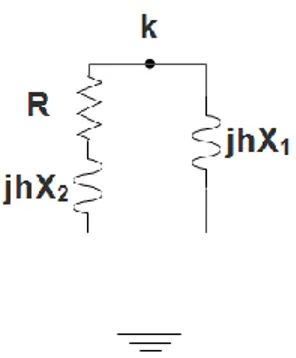
Figure 2-14 Equivalent circuit for RL series load ... 30

Figure 2-15 Equivalent circuit of RL parallel ... 31

Figure 2-16 RL equivalent circuit of RL parallel with skin effect ... 31

Figure 2-17 Equivalent circuit of a CIGRE type C ... 32

Figure 2-18 Y connection of spot load ... 33

Figure 2-19 Delta connection of spot load ... 33

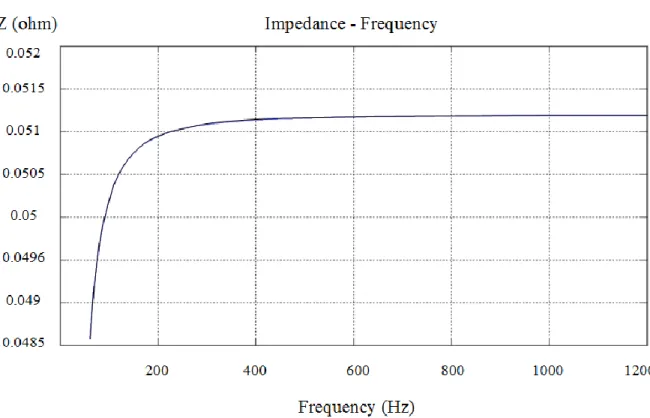
Figure 2-20 Impedance scan of RL series load (60 Hz < f < 1200 Hz) ... 34

Figure 2-21 Impedance phase of RL series load (60 Hz < f < 1200 Hz) ... 35

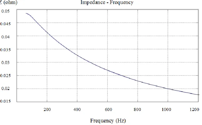
Figure 2-22 Impedance scan of RL parallel load (60 Hz < f < 1200 Hz) ... 35

(13)

Figure 2-24 Impedance scan of RL parallel load with skin effect (60 Hz < f < 1200 Hz) ... 36

Figure 2-25 Impedance phase of RL parallel load with skin effect (60 Hz < f < 1200 Hz) ... 37

Figure 2-26 Impedance scan of CIGRE type C (60 Hz < f < 1200 Hz) ... 37

Figure 2-27 Impedance phase of CIGRE type C (60 Hz < f < 1200 Hz) ... 38

Figure 2-28 Equivalent circuit of induction motor ... 39

Figure 2-29 Impedance scan of induction motor (60Hz < f< 1200 Hz) ... 42

Figure 2-30 Phase impedance of induction motor (60Hz < f< 1200 Hz) ... 42

Figure 2-31 Synchronous motor (Yg) ... 44

Figure 2-32 Synchronous motor (Delta or Y) ... 44

Figure 2-33 Impedance characteristic of synchronous machine (60 Hz < f<1200 Hz) ... 45

Figure 2-34 Phase impedance of the synchronous machine (60 Hz < f < 1200 Hz) ... 46

Figure 2-35 Nonlinear load ... 47

Figure 2-36 Norton equivalent of a nonlinear load ... 47

Figure 3-1 Single tuned filter ... 51

Figure 3-2 Impedance Scan of single tuned harmonic filter (tuned at 420 Hz) ... 51

Figure 3-3 High pass harmonic filter ... 52

Figure 3-4 Impedance Scan of High pass harmonic filter (tuned at1020 Hz) ... 52

Figure 3-5 C-Type harmonic filter ... 53

Figure 3-6 Multiple filter bank ... 53

Figure 3-7 Flowchart 1 of Passive Filter Design ... 64

Figure 3-8 Flowchart 2 of Passive Filter Design ... 65

Figure 3-9 Harmonic filter placement ... 68

Figure 4-1 IEEE 34 bus distribution system ... 70

(14)

Figure 4-3 Voltage waveform at Bus 880a (from MATLAB code) ... 74

Figure 4-4 Voltage waveform at Bus 880a (from MATLAB code) ... 76

Figure 4-5 5-Bus industrial system with multiple harmonic filters at bus 5 ... 80

Figure 4-6 Voltage waveform at bus 5 (from CYME Harmonic module) ... 82

Figure 4-7 Current waveform at bus 5(from CYME Harmonic module) ... 82

Figure 4-8 Voltage Individual Harmonic Distortions (Voltage IHD) ... 82

Figure 4-9 Voltage Total Harmonic Distortions (Voltage THD) ... 83

Figure 4-10 Current Total Harmonic Distortions (Current THD) ... 83

Figure 4-11 Impedance characteristic waveform before filtering at bus 5 (from CYME Harmonic module) ... 83

Figure 4-12 Voltage at bus 5 (from CYME Harmonic module) ... 85

Figure 4-13 Current waveform at bus 5(from CYME Harmonic module) ... 85

Figure 4-14 Voltage Individual Harmonic Distortions (Voltage IHD) ... 85

Figure 4-15 Voltage Total Harmonic Distortions (Voltage THD) ... 86

Figure 4-16 Current Total Harmonic Distortions (Current THD) ... 86

Figure 4-17 Impedance characteristic waveform after filtering at bus 5 (from CYME Harmonic module) ... 86

Figure 4-18 13 Bus industrial system ... 88

Figure 4-19 Voltage THD weight of the 13 bus system (before filters placement) ... 89

Figure 4-20 Voltage THD weight of 13 bus system (Filter at bus 4) ... 90

(15)

(16)

LIST OF SYMBOLS AND ABBERVIATIONS

(1.1) Equation 1.1

[1] Reference 1

Complex number

Dc MANA Dependency functions matrix V_N−LL Nominal line-to-line voltage

Id MANA Unknown currents in dependent voltage source vector

In MANA Nodal currents injection vector

Is MANA Unknown currents in zero impedance element vector

Iv MANA Unknown source current vector

SC MANA Adjacency matrix of zero impedance type devices Scc−1∅ Single-phase short-circuit power

Scc−3∅ Three-phase short-circuit power

SD MANA Adjacency matrix of infinite impedance type devices

Vibe MANA Voltage sources vector

Vic MANA Voltage sources adjacency matrix

Vn MANA Unknown node voltages vector

Yn MANA Linear network admittance matrix

Z0 Complex zero sequence impedance

Z1 Complex positive sequence impedance

Z2 Complex negative sequence impedance

Z012 Complex sequence impedance

Delta Ungrounded delta connection or system Y Wye ungrounded connection or system Yg Wye grounded connection or system

GMR Geometrical Mean Radius

THD Total Harmonic Distortion IHD Individual Harmonic Distortion

(17)

MANA Modified-Augmented-Nodal Analysis

p.u. Per-Unit

X/R Inductive per resistive ratio PCC Point of Common Coupling

PF Power Factor

(18)

LIST OF APPENDICES

Appendix A – DISTORTION FACTORS ... 101 Appendix B – COMMON VOLTAGE AND REACTIVE POWER RATING BASED ON IEEE 18 ... 102

(19)

CHAPTER 1 INTRODUCTION

1.1 Overview

Immediately upon, the electrical devices with nonlinear current-voltage characteristics such as power converters came into use in the 1970s; the ability of power system to control harmonic propagations has gained attention. However, concerns regarding the harmonic distortions were overlooked around that time, such that the harmonics in distribution systems could cause problems in the performance of network elements. Generally, the harmonics produced by nonlinear devices can reduce efficiency of the power system and in some cases it can even trip circuit breakers. In distribution networks, the end-user suffers from harmonic problems more than the utility sector does [1]. In industrial systems, since the adjustable speed drives, and the arc furnaces are close to each other, the problems caused by harmonic distortions are very likely to occur. Due to these facts, the harmonic propagations in distribution and power systems, particularly for industrial zones, should be precisely analyzed.

Since the power quality is significantly affected by propagation of harmonic distortions in power systems, harmonic control has become a critical issue. One of the most common methods to achieve harmonic distortion reduction is the use of harmonic filters. It should be noted that this reduction greatly depends on the filtering system placement. There are two types of harmonic filters commonly found in industrial systems (i) passive filters and (ii) active filters. The main difference of these filters stand on whether they cancel harmonic distortions within specific frequencies.

1.2 Objective

The main objective of this research project is to develop an algorithm for calculating harmonic voltages and currents in unbalanced networks so that the result can be used for resonance measurements and harmonic filter design. Although the proposed method is suitable for transmission systems or other highly meshed systems, the main focus of this work is on unbalanced distribution systems. The sub objective of this research project is to design and place suitable harmonic filters and accordingly reduce the propagation of harmonic distortions in industrial networks.

(20)

1.3 Methodology

According to the specific objective of this project, the present study includes using a mathematical method for determining the harmonic distortions. This method involves the modified augmented nodal analysis and is applied to steady state computations. Once all the system elements are modified into their harmonic models respectively, the developed MANA algorithm is employed for harmonic analysis. It should, nonetheless, be noted that the harmonic models of system elements due to their frequency-dependent nature can be very complex and demanding to obtain when high precision levels are targeted. Generally accepted, steady state models are considered in this work for the harmonic modeling of components. Regarding the metrics on the quality of power, the IEEE standard 519 is considered here as the main reference. The purpose of IEEE 519 standard is to make sure that the utility maintains a certain quality of power at the load terminals and that load is not subjected to high levels of harmonics [2]. Finally, the harmonic analysis is validated by using the IEEE 34 bus distribution test system. The validation test case demonstrates that the proposed algorithm yields precise results.

The secondary objective is related to the optimization of filter design and involves the use of two algorithms. The first algorithm is used to determine the parameters of the passive harmonic filters while respecting the limits set by IEEE 519 and IEEE 18. In this algorithm a systematic procedure to design the harmonic filters is used considering the use of all the passive filters available. It has to be mentioned that the application of passive harmonic filters is a common practice for suppressing harmonic propagations in industrial power systems because they can provide harmonic control and power factor correction simultaneously and also they are much cheaper than active filters. The second algorithm presents a simple strategy to find efficient locations of harmonic filters. A successful filter placement strategy should utilize the minimum number of filters to achieve the greatest positive impact on power quality of the system [3]. Since the number of buses allowing a filter installation in industrial systems is usually not exhaustive, it is possible to determine the optimum filter location by simulating all possible configurations. Although this is a brute force approach, given the performance of present day computers and the size of the industrial networks, it is not demanding in terms of CPU time and it provides guaranteed solution. The effectiveness of the algorithm, on the other hand, is demonstrated on a test case described in chapter 4.

(21)

1.4 Report outline

The present thesis is organized into five chapters.

Chapter 1 provides an overview of the research project and information on the objectives and the methodology used.

Chapter 2 presents an algorithm based on MANA for performing harmonic analysis; it also describes and gives insight on the parameters and advanced equivalent circuit models of all power system elements that can be encountered in typical harmonic studies.

Chapter 3 proposes an approach to design and place harmonic filters in the industrial networks. Chapter 4 presents validation test cases used for testing the presented solution methods.

Chapter 5 is the conclusions of this work. Based on the results, some recommendations and suggestions for future research work are presented.

1.5 Research Contributions

The major contributions of this thesis are listed as follows:

 The harmonic distortions in balanced and unbalanced networks are calculated using the state of the art MANA technique in phasor domain. The MANA approach is already demonstrated to perform for short circuit, power flow, state estimation and fault flow studies. Demonstrating that it can also be used for harmonic studies unifies the solver platform for all the steady state analysis in distribution systems.

 The multiphase harmonic models are presented all together so that they can be of use for harmonic studies.

 The phasor domain harmonic solutions are compared to EMTP-RV (Electromagnetic Transient Program) simulations.

 A systematic study to determine the size and type of harmonic filters in order to suppress harmonic distortions in industrial systems is presented.

 A systematic study to find efficient locations for harmonic filters in industrial power systems is demonstrated by taking into account the standards in effect.

(22)

CHAPTER 2 HARMONIC ANALYSIS IN UNBALANCED NETWORKS

The algorithm presented in this section is based on MANA; the same formulation is also applied to the study of resonant conditions. MANA was already used for unbalanced distribution systems and proved to be efficient [4]. In this section, the harmonic models of system components are also presented with their impedance scan with respect to frequency.

2.1 Literature review

The frequency-dependent behavior of system components plays a significant role in harmonic analysis. A concise review on the modeling and analysis of harmonic propagation in ac networks considering the frequency dependent behavior and along with practical considerations is presented in [5]. It should, however, be noted that synchronous machine is modeled using single phase units. Due to this fact, in three phase system, three single phase machines are connected; therefore, the mutual effects are neglected. Several harmonic models and harmonic analysis are described in [6] and [7]. The harmonic model of induction machine under balanced and unbalanced conditions is shown in [8]. The proposed model obtains the harmonic impedance for induction machine of all three sequences (zero, positive, and negative). The appropriate models of synchronous generators for harmonic studies are presented in [9]. These models are developed using detailed "dq0" representations of the synchronous machine. In [10] a synchronous machine model is developed for three-phase harmonic load flow analysis and for initialization of the EMTP-RV. This model can represent both the frequency conversion and the saturation effects under various machine load flow constraints. The model is in the form of a frequency-dependent three-phase circuit. It can therefore easily be incorporated into existing harmonic programs for system-wide harmonic analysis. In [11], a survey on a number of models for linear loads is demonstrated along with their impact on the harmonic impedance of the system.

In distribution systems the state of the art is to develop generic methods that can handle unbalanced networks. In [4], an algorithm based on MANA to calculate multiphase load flow in unbalanced distribution systems is presented. A bibliographical review of the harmonic load flow formulation under balanced condition is provided in [12] which consist of four methods, (i) Harmonic Penetration, which assumes no harmonic interaction between network and harmonic sources, (ii) Iterative Harmonic Penetration (IHP), which considers harmonic influence on

(23)

harmonic sources, however, the fixed-point iteration technique, Gauss-Seidel (GS), used in the IHP could present convergence problems, (iii) Simplified Harmonic Load Flow, in this method, A fixed-point iteration of two Newton–Raphson procedures is used: one for load flow and the other for harmonic analysis, (iv) Complete Harmonic Load Flow, this formulation is a natural modification of the load flow where the harmonic sources’ treatment and the harmonic voltage calculation have been included. It is based on the simultaneous resolution of power constraints, harmonic current balance, and harmonic source equations. In [13] a multiphase harmonic load flow technique is provided which solves the network at fundamental and harmonic frequencies. The procedure uses an iterative analysis. In [14] and [15] as well, iterative harmonic analysis techniques in frequency domain are presented. The use of Norton equivalent in harmonic analysis is detailed in [16]. A time domain technique is presented in [17]. Different methods for harmonic analysis in frequency domain and time domain are currently detailed in the literature. In [18] a concise yet detailed revision of theoretical fundamentals and principles of classical methods for harmonic analysis in time domain and frequency domain calculations are presented. In this paper, frequency and time domain methods have been developed with the purpose of combining the individual advantages of the frequency and time domain methods.

2.2 Harmonic

Harmonic is defined as a sinusoidal voltage or current that is an integer multiple of the fundamental frequency (60 or 50 Hz). For example, a 180 Hz sine-wave signal, superposed onto the fundamental 60 Hz mains frequency, is defined as the 3rd harmonic (3 x 60 Hz).

2.3 Inter-harmonic

Any signal component between each harmonic order is named as inter-harmonic. In some cases, inter harmonic may play significant role in the total harmonic distortion of a system; however in this work, inter harmonics are not taken into account.

2.4 Characteristics of harmonic

In general, the harmonic voltage at the terminals of an element is given by:

 

1

1sin( ) 2sin(2 2) 3sin(3 3) ...

cos(   )       n h n h V t V h t V t V t V t  



        (2.1)

(24)

Where

 

V t : Voltage at terminal h V

: Harmonic voltage at h harmonic order

h : Harmonic order

 _{: Angular frequency measured in radians per second}

n



: Phase shift

In a balanced three phase system, the phase shift between each phase is exactly 120 degrees. Thus, the waveform of 𝑉_𝑏 and 𝑉_𝑐 are 120 degrees and 240 degrees shifted from 𝑉_𝑎 respectively. The voltage at fundamental frequency is given by:

1cos(



0 ) a V V t (2.2) 1cos(



0 120) b V V t (2.3) 1cos(



0 120) c V V t (2.4) Where: 1

V : Voltage at fundamental frequency

a V : Voltage in phase a b V : Voltage in phase b c V : Voltage in phase c

Due to the symmetry, the harmonic voltage at fundamental frequency has only positive sequence (in balanced networks).

It should be noted that if the waveform is shifted by



_n, its harmonics are shifted by h



_n (h is harmonic order). Therefore, the second harmonic components of the three phase waveform are given by:

2cos(2



0 2 0)

a

(25)

2cos(2



0 2 120) 2cos(2



0 120) b V V t  V t (2.6) 2cos(2



0 2 120) 2cos(2



0 240) c V V t  V t (2.7)

Due to the phase shifts, the harmonic voltage at second harmonic order has only negative sequence.

Third harmonic components are given by:

3cos(3



0 3 0) a V V t  (2.8) 3cos(3



0 3 120) 3cos(3



0 0) b V V t  V t (2.9) 3cos(3



0 3 120) 3cos(3



0 0) c V V t  V t (2.10)

If we consider the third harmonic components, we can see that the phase shifts in all three phases are equal to zero degree. Therefore, all three terminals are equal in potential. And, accordingly voltage at third harmonic order has only zero sequence.

Eventually, the above reveals that fundamental, fourth, seventh and … harmonics have positive sequence, and they are named positive sequence harmonics. The second, fifth, eighth and … harmonics have negative sequence and they are named negative sequence harmonic. The triplen harmonics have zero sequence and they are named zero sequence harmonic.

2.5 MANA formulation

The MANA formulation is utilized for multiphase harmonic analysis and frequency scan. The generic formulation of MANA is given by:

A x = b (2.11)

Where:

𝐀 : System of equation 𝐛 : Known Variable of system 𝐱 : Unknown Variable of system The detailed format is given by:

(26)

0 0 0 . 0 0 0 0 0 0 0                  _                       h h n n c c c n t h b C V t h C D t h C d S I Y V D S V V V I D I S S I (2.12) Where:

𝒀𝒏 : Linear network admittance matrix 𝑽_𝒄 : Voltage sources adjacency matrix 𝑫_𝒄 : Dependency functions matrix

𝑺𝒄 : Adjacency matrix of zero impedance type devices 𝑺_𝒅 : Adjacency matrix of infinite impedance type devices 𝑽𝒏 : Vector of unknown nodal

𝑰𝒗 : Vector of unknown voltage source currents

𝑰_𝒅 : Vector of unknown currents in dependent branch functions 𝑰_𝒔 : Vector of unknown currents in zero impedance element vector 𝑰𝒏 : Vector of nodal current injections

𝑽_𝒃 : Vector of known source voltages

2.6 Impedance scan (Frequency scan)

An impedance scan, also known as frequency scan is used to identify the resonance conditions in the system. In this approach, unit current is injected to the network then the calculated voltage gives the driving point impedance. A plot of magnitude of driving point impedance versus frequency provides an indication of the resonance condition. A sharp rise in the impedance implies parallel resonance which gives the maximum impedance; on the other hand, the lowest point of the impedance scan identifies series resonance.

(27)

2.7 Harmonic analysis

The harmonic analysis is the procedure used for obtaining the harmonic voltages in electric power systems at harmonic frequencies. This procedure can be either performed using time domain tools or frequency domain tools. The time domain tools provide higher levels of sophistication with circuit based modeling options and higher precision [19]. However, less computation time is required in frequency domain tools, and reasonable accuracy for practical applications is usually achievable. Therefore frequency domain solution is widely adopted for harmonic studies. In this work only the frequency domain solution is considered. As the objective is to study unbalanced networks using a general and flexible approach, the MANA method is selected to obtain the system of equations for harmonic analysis. In balanced three phase systems, under balanced operating conditions, harmonics on each phase are related to other phases with specific equations (refer to the characteristics of harmonics). As mentioned before, the triple harmonics appear as zero sequence components. As such, in grounded wye configurations, these harmonics flow in the lines and neutral/grounding circuits, while in delta or ungrounded systems they cannot exist. Similar analysis shows that the fifth harmonic appears as negative sequence, seventh as positive sequence, etc. therefore, the impedances and the connection types of rotating machines, transmission lines, and transformers should be accounted for [5]. Under unbalanced conditions, the three phase voltages at the terminals of the loads are not symmetrical; consequently, propagation of harmonics is more complex and a general multiphase solution technique such as MANA is required.

Generally, harmonic studies in frequency domain consist of two steps: 1- Fundamental frequency load flow

2- Harmonic frequency steady state computation in which the loads are considered as constant impedances.

In this work both steps are performed using the MANA formulation. The MANA load flow formulation is used in the first step and it aims to determine the voltages and currents at fundamental frequency. The steady state MANA formulation is used in the second step and the objective is to obtain the harmonic voltages and currents at each bus at each harmonic frequency.

(28)

Another method used in harmonic studies is the Iterative Harmonic Analysis (IHA). In this method, loads are not modeled as constant impedance and, fixed point technique is performed to determine the proper value of load impedances at each harmonic frequency. In some cases, IHA may present convergence problem. Due to this fact, the steady state computation is recommended.

2.7.1 Algorithm of harmonic analysis

The algorithm of harmonic analysis is as follows:

Step 1 - Initialization

 Determine voltage and current at fundamental frequency using MANA load flow formulation [4].

Step 2 – Build MANA matrix for steady state computation of network

 Identify the harmonic order

 Short circuit the voltage sources, and modify into the equivalent impedance

 Modify nonlinear loads into the Norton equivalent load models at harmonic frequency (refer to modeling of network component) (Figure 2.2)

 Modify network elements into harmonic models at harmonic frequency (refer to modeling of network component) (Figure 2.1)

 Construct and solve the following equation (MANA steady state computation)

0 0 0 0 0            _                   h h h n c c n n t h c d t h c d s Y D S V I D I S S I (2.13) Where: h n

I : Harmonic current (harmonic source)

Step 3 – Repeat step 2 for all harmonic frequencies

Result: harmonic voltages at each bus, harmonic currents at transformers and harmonic current through switches.

(29)

Figure 2-1Circuit in fundamental frequency

(30)

2.7.2 Flowchart of harmonic analysis

Figure 2-3 Flowchart of harmonic analysis

2.8 Iterative harmonic analysis (IHA)

There are various approaches to determine the harmonic distortions based on iterative calculations. The simplest one uses the concepts of fixed point or Gauss. In this method, harmonic influence on behavior of nonlinear devices is taken into account.

The algorithm of Iterative Harmonic Analysis (IHA) is very similar to the algorithm of harmonic analysis (direct analysis based on MANA), however, the steady state computation of harmonic analysis is complemented by iterative analysis.

(31)

Once the calculation of the voltages at fundamental frequency based on the load flow is reached, the linear devices of the network is modified into their harmonic models and the system is reduced to the nonlinear loads. Then afterward, at each iteration, the latest values of distorted terminal voltages are employed to determine the harmonic current injection by solving the linear system with Gauss – Seidel algorithm [6]. Eventually, the direct analysis (steady state computation) is used to calculate the harmonic voltages. It should be mentioned that this method can present the convergence problem [12]. The algorithm of IHA is presented in Figure 2-4.

Figure 2-4 Iterative Harmonic Analysis algorithm

2.9 Harmonic modeling of the network elements

The harmonic models of the system elements are given in this section.

2.9.1 Overhead line

There are many approaches to determine the impedance matrices of the distribution and transmission line due to the earth return model and the frequency interest. The first approach to model overhead line that included the effect of earth return was published in 1926 [20]. This line model is known as full Carson line model. However, over the years, the calculation procedures of the Carson model have been simplified. Both the simplified Carson model and full Carson model are detailed in Kersting’s book [21].

(32)

Carson line model

The calculation procedure for two conductors is presented in Figure 2-5. The self and mutual impedance of each conductor is calculated from the conductor i and k, and their images i’ and k’.

Figure 2-5 Phase conductors and images

Due to effect of earth return, correction factor should be applied to the computation of self and mutual impedances. This correction factor can be calculated as:

2 2 2 3 4

1 2 cos 3 cos 4

cos cos 2 cos 2 0.6728 ln sin 2

8 3 2 16 16 16 45 2 1536       _  _     π k k k k θ πk θ P k θ θ θ θ θ k (2.14) Where 𝑘 and 𝜃 are defined as:

3 1.713 10   _i f k h ρ (2.15) 0  θ (2.16) 2 3 4

1 2 1 cos 2 cos 3 sin 4 2

0.0386 ln cos (ln 1.0895)

2 3 2 64 45 2 384

    πk θ k θk θ θ 

Q k θ

k k (2.17)

Where 𝑘 and 𝜃 are defined as:

3 0.8565 10

  _ik f

k D

(33)

1 cos (  )  i k ik h h θ D (2.19)

The simplified model is provided as follows:

8 π P (2.20) 1 2 0.0386 ln 2    Q k (2.21)

As can be seen, in simplified method, the function of variable 𝜃 is ignored.

The self-resistance and self-inductive reactance of each conductor can be determined as: 4   ii c R R ωPG (2.22) 2 2 ln( ) 4   i  ii int i h X X ωG ωQG r (2.23) where 2 ln( )  i int i r X ωG GMR (2.24)

The self and mutual impedance of the transmission line based upon Carson line model are obtained from following equations:

ii i ρ Z f R f f j GMR f c 1 1 ( ) 0.00158836 0.00202237 1 ln 7.6786 ln 2       _   _{ }  _{ }_       (2.25) ik ik ρ Z f f f j D f 1 1 ( ) 0.00158836 0.00202237 1 ln 7.6786 ln 2           _  _{ } _{ }_       (2.26)



2 2



k 2 k 2 ( )     ij i i D x x y y (2.27) where:

Zii : Self-impedance of conductor i in Ω / mile

Zik : Mutual-impedance of conductor i in Ω / mile

Ri : Resistance of conductor i in Ω / mile f : System frequency in Hz

(34)

Dik : Distance between conductors i and j in ft.

𝜌 : Resistivity of earth in Ω / meters (assume 100 Ω / meters) 𝑅𝑐 : DC resistance at 25 C in Ω

𝑥_𝑖 : Horizontal distance between conductors in ft 𝑦𝑖 : Veridical distance between conductors in ft 𝐺 : Multiplying factor (0.1609347 x 10-3 ohm/mile) 𝑅_𝑖𝑖 : Self-resistance of the conductors

𝑋𝑖𝑖 : Self-inductive reactance

Deri line model

Deri equations for self and mutual impedance of a distribution or transmission line are obtained from the simplification to the full Carson line model. It should be taken into account, the simplified Carson has some convenient approximations for limited range of frequencies and medium frequencies are not covered. On the other hand, Deri approach results in simple formulas which are valid throughout, from very low frequencies up to several MHz [22]. Thus, Deri line models are employed in the harmonic studies of the lines. Deri line model is provided by using:

0 1 1 ( )   p σ ρ jωμ σ (2.28)



2 2



1   c e i i σ π r r R (2.29) 0 1  c c p j ω μ σ (2.30) 1 2  c e c Z π σ r p (2.31) 1 ( ) ( 2)  n  n _n  c Z R Z n (2.32) i ii c e μ h p Z jω Z π r 0 _ln2( ) 2    (2.33) i k ik ij i k ik h h p d μ Z jω π _h _h _d 2 2 0 2 2 ( 2 ) ln 2 ₍ ₎       (2.34)

(35)

Where:

Zii : Self-impedance of conductor i in Ω / km

Zij : Mutual-impedance of conductor i in Ω / km

Ri : Resistance of conductor i in Ω / km

𝜔 : 2𝜋 × 𝑓

ℎ𝑖 : Heights of the conductors i above the ground in meter ℎ_𝑘 : Heights of the conductors’ k above the ground in meter

𝜇0 : 4π × 1e − 7

f : System frequency in Hz 𝑑𝑖𝑘 : Horizontal separation in meter 𝑟_𝑒 : External radius in meter 𝑟𝑖 : Internal radius in meter 𝑅_𝑖 : DC resistance at 25 Hz in Ω

The most difference in the line impedance matrices of the simplified Carson, full Carson and Deri approaches is coming from difference assumptions for internal impedance of the conductors and handling of the conductor GMR [23].

The equivalent impedance matrix of the line calculated by Carson or Deri formula is given by: ( ) ( ) ( ) ( ) ( ) ( ) ( ) ( ) ( ) ( ) ( ) ( ) ( ) ( ) ( ) ( ) ( )              abcn Z f aa ab ac an ba bb bc bn ca cb cc cn na nb nc nn Z f Z f Z f Z f Z f Z f Z f Z f Z f Z f Z f Z f Z f Z f Z f Z f (2.35)         _ _          _ __{ } _                   __ _{ } __ ' ij in abc abc _abc ' n ng _ng nj nn Z Z V V _I I V _V _Z _Z (2.36)

After Kron’s reduction, the equation is given by:

1



 _ _ _  _ 

     

(36)

( ) ( ) ( ) ( ) ( ) ( ) ( ) ( ) ( ) ( )            abc Z f aa ab ac ba bb bc ca cb cc Zs f Zs f Zs f Zs f Zs f Zs f Zs f Zs f Zs f (2.38) series( ) abc( ) Z f Z f (2.39)

Several effects which are normally ignored at power frequencies have to be included at harmonic frequencies, for instance [24]:

 Frequency dependence

 Long line effects

 Line impedances

 Line transpositions

 VAR compensation plant

In this section frequency dependence, long line effects and line impedances are explained. Line transpositions and VAR compensation plant are detailed in [24]. For calculation of transmission line parameters in harmonic frequencies, following theories should be covered:

 Evaluation of lumped parameters or PI model

 Evaluation of distributed parameters or distributed model

 Evaluation of Skin effect in transmission lines

1- PI (lumped parameters)

Figure 2-6 presents the equivalent circuit of PI. This model consists of series impedance and shunt capacitance which is divided into two equal parts and placed at the two ends of the line. The shunt capacitance of the line is computed as follows:

(37)

1 l ˆ _n ₍ ₎ 2   ii ii i S mile P πε RD μF (2.40) 1 ln ( ) 2 ˆ _ _ ij ij ij S _mile P πε D μF (2.41) i 2   ii S y (2.42) 2 2 (( ) ( ) )   ij ij ii S D S (2.43) n n 2 2 (( ) ( ) )      in i i S x x y y (2.44) where

Pii : Self-impedance of conductor i in Ω / mile

Pij : Mutual-potential coefficients of conductor

Sii : Distance from Conductor i to its image. (ft.)

Sii : Distance from Conductor i to the image of Conductor j (ft.)

Sin : Distance from Conductor i to the image of Neutral (ft.)

RDi : Radius of Conductor i in ft.

Dij : Distance from Conductor i to Conductor j (ft.) 𝜀 : Permittivity of air (Assume 1.4240 × 10−2₍ 𝜇𝐹

𝑚𝑖𝑙𝑒) ) ˆ ˆ ˆ ˆ ˆ ˆ ˆ ˆ ˆ ˆ ˆ ˆ ˆ ˆ ˆ ˆ        _{  } _         primitive P aa ab ac an ba bb bc bn ca cb cc cn na nb nc nn P P P P P P P P P P Z P P P P P (2.45) in ˆ ˆ ˆ ˆ ˆ P   _{  } _    _{ }  _{ }_ _{ } __       ij primitive nj nn P P P P (2.46)

Kron’s reduction is applied to obtain:

1                Pabc_{      } Pij Pin Pnn _Pnj_ (2.47) 1       Cabc  Pabc (2.48)

(38)

1 2 1.609344 ( )          Yabc j πf Cabc l μS (2.49) where 𝑓 : Frequency in Hz l : Length in km

2- Equivalent PI (distributed parameters)

Due to standing wave effect on voltage and current in long line, a number of PI models (lumped parameters) are connected in series to improve accuracy of voltage and current. According to the power system harmonic book written by Arrilaga, three phase PI model can provide accuracy to 1.2% for quarter wavelength line (a quarter wavelength corresponds with 1500 and 1250 km at 50 and 60 Hz respectively). As frequency increase the number of nominal PI section to maintain a particular accuracy increases proportionally. For instance, a 300 km line requires 30 nominal PI section to maintain the 1.2% accuracy [6]. Therefore, the long line effect should be included. And, the line parameters are distributed along the length of the line in a way to avoid lumping them in one place. In distributed model, the equivalent PI model (distributed parameters) is calculated from the PI model (lumped parameters) by multiplying the correction factors to the series impedance and shunt admittance. For the single phase the correction factor is given by: For series impedance:

` ` ` ` sinh(x Z Y )

x Z Y

(2.50) For shunt admittance

` ` ` ` tanh( ) 2 2 x Z Y Z Y x (2.51) where

𝑥 : Length of the line

𝑍` _{: Series impedance calculated in PI nominal in Ω/km}

(39)

Since there is no direct way of computing sinh or tanh of a matrix, eigenvalues and eigenvectors are employed for three phase line models.





 Z_abcY_abc v T eig (2.52)





 Y_abcZ_abc i T eig (2.53) 1     m abc Z T_v Z T _i (2.54) 1     m abc Y T_i Y T _v (2.55)





  m m m Γ diag Z Y (2.56)  T T i v T T (2.57)

 

1 1 ( ) ( )  sinh( )  series abc m m Z f Z f T _iΓ diag Γ l T _i (2.58)

 

1 1 ( ) 2 h( ) ( ) 2 tan      shunt m m abc Y f T _iΓ diag Γ l T_i Y f (2.59) where 𝑓 : Frequency in Hz1

𝑍𝑎𝑏𝑐 : Series impedance calculated in PI nominal in Ω/km

𝑌_𝑎𝑏𝑐 : Shunt admittance which is calculated in PI nominal in 𝛺−1_/km 𝑍_{𝑠𝑒𝑟𝑖𝑒𝑠} : Series distributed impedance in 𝛺

𝑌𝑠ℎ𝑢𝑛𝑡 : Shunt distributed impedance in 𝛺

The use of PI model (lumped parameters) at fundamental frequency can offer several advantages:

 It requires lowest calculations and is easy to be implemented.

 It can be used in any configuration or number of parallel circuits.

 It can be used in the simulation related to transient or dynamic processes. Moreover, PI model (lumped parameters) has some disadvantages:

 There are considerable errors in the use of lumped parameter when the transmission length is greater than 150 km at fundamental frequency (50 or 60 Hz) and 15 km at 600 Hz. Therefore, transmission lines cannot be represented with PI (lumped parameters) at harmonic frequencies.

(40)

 PI model does not represent frequency dependence on R and L in the case of studies related to the frequency response or harmonics [25].

Equivalent PI (distributed parameters) must be used in any study where the frequency changes are relevant to the results such as harmonic analysis [25].

3- Skin Effect

In transmission lines, the current flowing tends to flow on the surface of the conductor. Due to this fact, there is an increase in the resistance and decrease in internal inductance. This effect increases as frequency increases and it is termed the skin effect [6].

The skin effect in transmission lines is explained in [6] and [24]. The equation of skin effect is provided as follows: 2 0    skin ll Z R Z (2.60) 0 2 2 , , 1 ( )   ext l int l c R π r r δ (2.61) 0 2 2 , , 1 ( )   ext l int l c R π r r δ (2.62) , 1 2   ext l c C Z πr δ ρ (2.63) 0 1  C c ρ jωμ δ (2.64) where

𝑟_{𝑖𝑛𝑡,𝑙} : Internal radius of the conductor l in m 𝑟𝑖𝑛𝑡,𝑙 : External radius of the conductor l in m 𝛿_𝑐 : Conductivity of the conductor in S/m

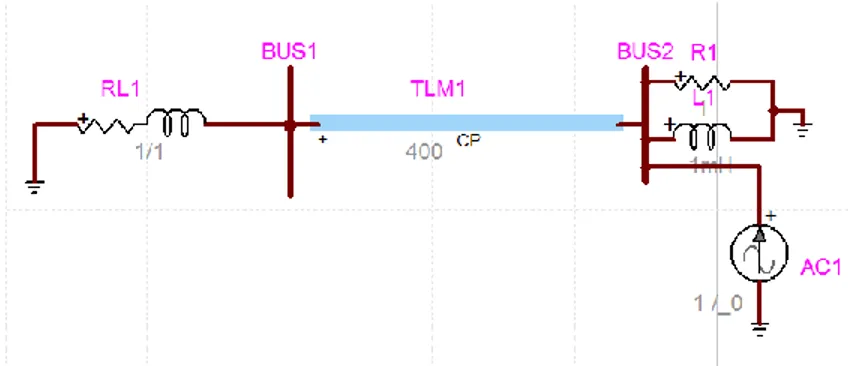
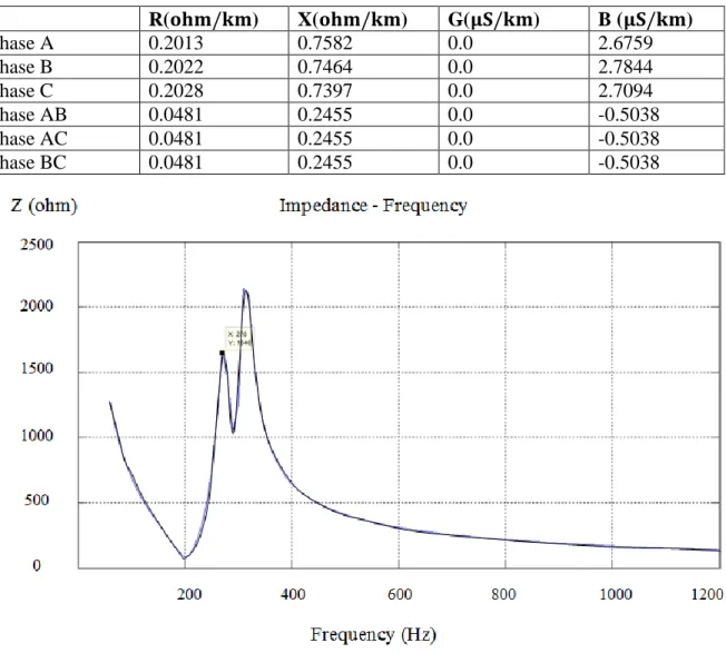
The impedance scan of a transmission line with different harmonic models are presented in Figures 2.7 to 2.12; the line length is 300 km and Deri equation is used to calculate the series impedance of the line. Table 2-1 shows the line parameters data at fundamental frequency.

(41)

Table 2-1 Line parameters data (in 60 Hz) R(𝐨𝐡𝐦/𝐤𝐦) X(𝐨𝐡𝐦/𝐤𝐦) G(𝛍𝐒/𝐤𝐦) B (𝛍𝐒/𝐤𝐦) Phase A 0.2013 0.7582 0.0 2.6759 Phase B 0.2022 0.7464 0.0 2.7844 Phase C 0.2028 0.7397 0.0 2.7094 Phase AB 0.0481 0.2455 0.0 -0.5038 Phase AC 0.0481 0.2455 0.0 -0.5038 Phase BC 0.0481 0.2455 0.0 -0.5038

(42)

Figure 2-8 Real part of a PI nominal line (60Hz <f<1200 Hz)

(43)

Figure 2-10 Impedance characteristic of a distributed line (equivalent PI) (60Hz <f<1200 Hz)

(44)

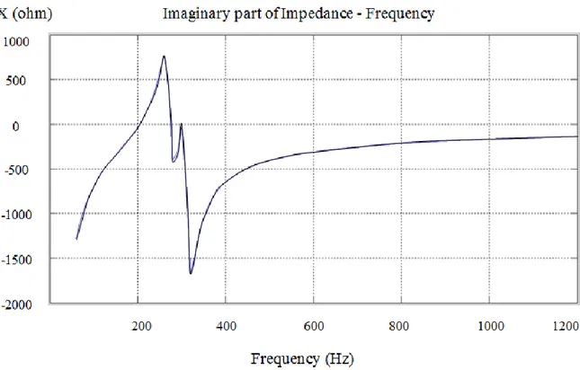
Figure 2-12 Imaginary part of a distributed line (equivalent PI) (60Hz <f<1200 Hz)

2.9.2 Cable

The harmonic model of cables is very similar to overhead lines. However, cables have higher shunt capacitance than overhead lines [5]. Therefore, the equivalent PI model (distributed parameters) can be applied for cables.

2.9.3 Voltage sources

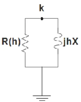
At harmonic frequencies, the sources are grounded and represented by lumped impedance; the equivalent admittance matrix of the source is constructed by:

R jX h    h a Z (2.65) 1 [ ]      _{ }      h h source abc Y Z h h h x y z h h h z x y h h h y z x Y Y Y Y Y Y Y Y Y (2.66) Where R : Resistance of source

(45)

X : Reactance of source

𝑍(ℎ) : Harmonic impedance of the source in ohm

ℎ : Harmonic order

𝒀_𝒏 is a 2n x 2n matrix for n phase line:

     _{ } _     h n source Y Y h h h x y z h h h z x y h h h y z x Y Y Y Y Y Y Y Y Y (2.67)

2.9.4 Transformers

The transformers at harmonic frequencies are represented with constant RL branches. The equivalent circuit is shown in Figure 2-13. The frequency dependence is usually ignored as the harmonic frequencies cover a small range frequency band. The nonlinear characteristics of the magnetizing branch and winding stray capacitance tend to produce harmonic distortions (mainly 3rd). Consequently, a harmonic source can be used to represent these distortions, although the effect is often negligible.

The harmonic impedance of transformers is modified with following equation:

 

  

Z h R jX h (2.68)

Where

R : Resistance of transformer

X : Reactance of transformer

The admittance matrix of the transformer in general format can be computed using:

1 0 0 0 0 0 0             Y Z Z Z (2.69)

(46)

Figure 2-13 Yg yg transformer

The equivalent admittance of Ygyg transformer shown in figure 2.13 is given by:

_ 1 _ 1 _ 2 _ 3 _ 1 _ 2 _ 3 n 0 0 0 0 0 0 0 0 0 0 0 0 0 0 0 0 0 0 0 0 0 0 0 0 0 0 0 0 0 0 0 0 0 0 0 0 0 0 0 0 0 0 ₀ ₀ ₀ 0 0 0 ₀ ₀ ₀ Y  a b c a a b c a b c sHX mHX mHX sHX a sHX mHX mHX mHX b sHX mHX mHX mHX c sHX mHX mHX s a sHX mHX b mHX sHX c mHX mHX m m m n k _k _k k k k Y Y Y -Y m Y Y Y -Y m Y Y Y -Y m -Y -Y -Y Y n -Y -Y n -Y -Y n -Y -Y o p _ 2 _ 3 _ 1 _ 2 _ 3 0 0 ₀ ₀ 0 0 ₀ ₀ 0 0 ₀ ₀ 0 0 0 0 0 0 0 0 0 0 0 0 0 0 0 0 0 0 0 0                                       b c mHX mHX sHX mHX sHX mHX HX mHX mHX sHX mHX mHX sHX mHX mHX Hg Xg n n _o _p -Y -Y -Y -Y -Y -Y Y Y Y Y Y Y Y Y Y Y (2.70) Where _ sHX i

Y : Self admittance seen on the low side for unit i, i = 1, 2, 3

Hg

Y : Grounding admittance for high side

Xg

Y : Grounding admittance for low side

Three phase power transformer can also give a phase shift to harmonic voltages and currents. The matrix Dc accounts for it in the MANA formulation

(47)

1 2 3 1 2 3 1 2 3 0 0 0 0 0 0 1 0 0 0 1 0 0 0 1 1 1 1    _        _                  _ _ _    c D a b c a b c q q q k g k g k g m m m o g g g p (2.71) Where

𝑔𝑖 : Turn ratio of the ideal transformer i, i = 1,2,3

2.9.5 Loads

Loads may either significant affect in damping or resonance conditions of the systems, particularly at higher frequencies. Harmonic modeling of linear loads is related to (i) load size (ii) composition and (iii) connection types. A typical composition of ordinary loads is presented in Table 2-2. There are three types of loads: 1- Spot loads (Resistive) 2- Rotating loads (inductive) 3- Nonlinear loads (harmonic sources)

Table 2-2 Typical load composition [9]

Nature Type of loads Electrical Characteristics

Domestic Incandescent lamps Spot load (Resistive)

Commercial Fluorescent lamps Nonlinear loads (harmonic

sources)

Industrial

Motors Rotating loads (inductive)

Computers Nonlinear loads (harmonic

sources)

Home electronics Nonlinear loads (harmonic

sources)

Resistive heater Spot loads (Resistive)

Air conditioning Rotating loads (inductive)

ASDs Nonlinear loads (harmonic

sources)

Pumps Rotating loads (inductive)

A Novel Approach to Determine Harmonic Distortions in Unbalanced Networks and Harmonic Filter Planning in Industrial Systems

DEDICATION

ACKNOWLEDGMENTS

RÉSUMÉ

ABSTRACT

TABLE OF CONTENTS

LIST OF TABLES

LIST OF FIGURES

LIST OF SYMBOLS AND ABBERVIATIONS

LIST OF APPENDICES

CHAPTER 1

INTRODUCTION

1.1 Overview

1.2 Objective

1.3 Methodology

1.4 Report outline

1.5 Research Contributions

CHAPTER 2

HARMONIC ANALYSIS IN UNBALANCED NETWORKS

2.1 Literature review

2.2 Harmonic

2.3 Inter-harmonic

2.4 Characteristics of harmonic

 



 

































2.5 MANA formulation

2.6 Impedance scan (Frequency scan)

2.7 Harmonic analysis

2.7.1 Algorithm of harmonic analysis

2.7.2 Flowchart of harmonic analysis

2.8 Iterative harmonic analysis (IHA)

2.9 Harmonic modeling of the network elements

2.9.1 Overhead line





















 

 

2.9.2 Cable

2.9.3 Voltage sources

2.9.4 Transformers

 

2.9.5 Loads