HAL Id: hal-00770596
https://hal.inria.fr/hal-00770596v2
Submitted on 28 Feb 2013
HAL is a multi-disciplinary open access
archive for the deposit and dissemination of
sci-entific research documents, whether they are
pub-lished or not. The documents may come from
teaching and research institutions in France or
abroad, or from public or private research centers.
L’archive ouverte pluridisciplinaire HAL, est
destinée au dépôt et à la diffusion de documents
scientifiques de niveau recherche, publiés ou non,
émanant des établissements d’enseignement et de
recherche français ou étrangers, des laboratoires
publics ou privés.
Localization of Single Link-Level Network Anomalies:
Problem Formulation and Heuristic
Emna Salhi, Samer Lahoud, Bernard Cousin
To cite this version:
Emna Salhi, Samer Lahoud, Bernard Cousin. Localization of Single Link-Level Network Anomalies:
Problem Formulation and Heuristic. [Research Report] 2013. �hal-00770596v2�
Localization of Single Link-Level Network
Anomalies: Problem Formulation and Heuristic
Emna Salhi
University of Rennes 1 IRISA, France [email protected]Samer Lahoud
University of Rennes 1 IRISA, France [email protected]Bernard Cousin
University of Rennes 1 IRISA, France [email protected]Abstract—Achieving accurate, cost-efficient, and fast anomaly
localization is a highly desired feature in computer networks. A necessary and sufficient condition on the set of paths that need to be monitored upon detecting a single link-level anomaly in order to localize its source unambiguously have been established. However, this paper demonstrates that this condition is sufficient but not necessary. A necessary and sufficient condition that reduces the localization overhead, cost and delay significantly, as compared to the existing condition, is established. Furthermore, an ILP algorithm that selects monitoring paths and monitor locations which satisfy the established condition jointly, thereby enabling a trade-off between the number and locations of mon-itoring devices and the quality of monmon-itoring paths, is devised. The problem is shown to be N P-hard through a polynomial-time reduction from the N P-hard facility location problem, and therefore, a scalable near-optimal heuristic is proposed. The effectiveness and the correctness of the proposed anomaly localization scheme are verified through theoretical analysis and extensive simulations.
Index Terms—Network monitoring, network diagnosis, anomaly
localization, anomaly detection, link-level anomalies.
I. INTRODUCTION
Anomaly localization aims at identifying unambiguously the link that causes an anomalous behavior of the network (e.g. excessive delay, high packet loss rate, etc.). Recent research works argued that continuous anomaly localization results in high overhead on the underlying network, and hence, is likely to interfere with the network services . Subsequently, most recent monitoring schemes proceed in two phases (e.g. [1] [2] [3] [12] [13] [14] [15]). The first phase, the detection phase, uses as few network resources as possible to only detect anomalies. A necessary and sufficient condition to detect all link-level anomalies is to cover all links of the network. Upon detecting an anomaly, the detection phase returns a set of suspect links. The localization phase is triggered then. It aims at reducing the set of suspect links to the anomalous link(s). Clearly, this reactive anomaly localization approach reduces significantly the monitoring overhead compared to the continuous anomaly localization approach. However it presents a serious challenge: the localization must be as fast as possible, in order to enable a fast recovery of the network. Agrawal et al. [1] proposed an accurate link-level anomaly This work was supported by Alcatel-Lucent Bell Labs, France, under the grant n. 09CT310-01
localization scheme that can localize all potential single link-level anomalies in a given network. The key idea is to deploy resources that enable the monitoring of a set of paths that distinguishes all links of the network pairwise. Two links are said to be distinguished from each other if we are able to decide which one is anomalous when an anomaly occurs on one of them. Whenever an anomaly is detected, this set of paths is monitored in order to pinpoint the anomalous link. This technique is suboptimal in that it considers all the network links as suspect, ignoring the information provided by the detection process, which generates unnecessary overhead and delays the localization. More recently, Barford et al. [2] proposed another scheme that selects paths that are to be monitored during the localization phase. Although this technique minimizes the localization overhead, because the monitored paths distinguish only between the suspect links pairwise, it suffers from two imperfections. The first is the non-negligible time of computing the set of paths that are to be monitored upon detecting an anomaly, which increases the localization delay (i.e., time elapsed between the moment when an anomaly is detected and the moment when the anomalous link is pinpointed). The second is that there is no guarantee to localize all potential anomalies, because the deployed monitors ensure only the coverage of links1. In this paper, we demonstrate that 1) not all links of the network need to be distinguishable pairwise for localizing any potential anomaly, 2) all potential anomaly scenarios can be derived offline from any detection solution that covers all the network links. Thus, we compute full and cost-efficient localization solutions, i.e., monitors that are to be activated and paths that are to be monitored upon detecting an anomaly, for all potential anomalies offline. Subsequently, we achieve an important gain in the localization delay and overhead.
Multiple works propose to compute the set of paths that are to be monitored dynamically upon detecting an anomaly (e.g., [4]-[10]). Practically, this means that one probe that maximizes the information gain given the previous probe observations is selected and sent in the network at a time. Such an approach is practical for highly dynamic environments. However, it is not practical for networks where anomalies are rare events, 1The monitors used for anomaly detection are deployed such that all the network links are covered by at least one monitoring paths. They can not necessarily localize all potential anomalies
especially, because it yields excessive delays.
Furthermore, most existing works consider only one crite-rion for monitoring path selection that is the minimization of the number of monitored paths, and only one criterion for monitor location selection that is the minimization of the number of deployed monitoring devices (e.g., [2] [1]). However, these criteria do not reflect the localization cost properly. Indeed, to reduce the localization delay and over-head, monitoring of links that do not provide extra localization information during the localization phase must be avoided. Moreover, monitor locations must be selected carefully to-wards minimizing the delay of communications between the Network Operation Center (NOC) and the deployed monitors. A novel anomaly localization cost model that considers the infrastructure cost, the localization overhead and the local-ization delay is, therefore, proposed. Besides, our anomaly localization scheme selects monitor locations and monitoring paths jointly, thereby enabling a trade-off between the number and locations of deployed monitoring devices and the quality of selected monitoring paths. We formulate the problem as an ILP, and we show that it is N P-hard through a polynomial-time reduction from the facility location problem.
Prior works on anomaly localization propose greedy ap-proaches for computing localization solutions (e.g., [1], [2], [11], [12]). In order to ensure the scalability, the number of candidate monitoring paths should reduced to a small subset of the network paths. Unfortunately, none of these works described how candidate monitoring paths are selected, however, the choice of candidate paths has a great impact on the quality of the localization solution. In this work we propose a heuristic that implements our anomaly localization scheme. We devise an efficient algorithm for candidate path computation that makes the heuristic scalable and near-optimal at a time. The key idea is to use a mathematically proven properties that enable us to find the best candidate monitoring paths between two given monitor locations by exploring a very small proportion of the network paths.
We verify the effectiveness of our anomaly localization scheme through extensive simulations and by comparing it with an hybrid anomaly localization scheme that combines the strengths of the scheme proposed in [1] and the scheme proposed in [2].
II. NETWORKMODEL ANDPROBLEMSTATEMENT We model the network as an undirected graphG = (N , E) comprising a set of nodesN connected by a set of undirected links 2 in E. Let P be the set of all non-looping paths of the network. Unless otherwise mentioned, without loss of generality, we assume that all paths in P are candidate to be monitored and all the network nodes are candidate to support monitoring devices. We use the term monitoring paths to designate paths that are monitored during the detection phase, also referred to as detection paths, or during the localization phase, also referred to as localization paths. We consider that 2This work can be easily applied for directed links. Each directed link is duplicated into
a network path is a set of links, instead of a sequence of links, and therefore, we apply set operations (e.g.,∩, ∪) on paths. We denote the anomaly detection solution by (Dm,Dp).Dmis the set of monitor locations where to deploy monitoring devices. Dp is a set of monitoring paths between the selected monitor locations that covers all the network links, ∪p∈Dpp = E. Furthermore, We note that we use the vertical bar notation to denote both set cardinality and absolute value.
We consider separable anomalies (e.g., connectivity, high-low loss model, delay spike model, etc) that satisfy the folhigh-low- follow-ing property: a path experiences an anomaly if and only if at least one of its constituent links is anomalous [16]. According to this property all links that are traversed by at least one detection path not exhibiting an anomaly are not anomalous, and all paths crossing an anomalous links exhibit the same anomaly. The remaining links constitute the set of suspect links. Anomaly localization aims at reducing the set of suspect links, inferred upon detecting an anomaly from the detection information, to the anomalous link. This requires monitoring additional paths that can distinguish between suspect links pairwise. Two links are said to be distinguishable from each other if we are able to decide which one is anomalous when an anomaly occurs on one of them.
The objective of this work is to come up with a localization scheme that enables the localization of all potential link-level anomalies accurately; while minimizing the cost of acquiring and deploying monitoring devices, the localization overhead and the localization delay. Our localization scheme infers all potential anomaly scenarios from any detection solution that covers all links of the network. This has two major benefits. The first is that we do not need to monitor a set of paths that can distinguish between every single pair of the network links whenever an anomaly is detected. The second is that we pre-compute full localization solutions for all anomaly scenarios offline, thereby accelerating the localization process. The inputs into our localization problem are an instance of the graphG = (N , E) and a set of detection paths Dp that covers all links in E, and the outputs are a set of monitor locations whose monitors are to be activated and a set of paths that are to be monitored for each potential anomaly. The localization solution must achieve a good trade-off between the monitor deployment cost, the localization overhead and the localization delay. To this end, a novel cost model that measures these three metrics is proposed. Also, our localization scheme selects monitor locations and localization paths jointly; as opposed to existing schemes that apply a two-step selection procedure, therefore omitting the trade-off between the number and locations of monitors and the quality of localization paths.
III. NOT ALL LINK PAIRS NEED TO BE DISTINGUISHABLE FOR LOCALIZING ANY SINGLE LINK-LEVEL ANOMALY In this section, we first establish a necessary and sufficient condition to distinguish between two links. Then, we prove that not all link pairs need to be distinguishable for localiz-ing any potential slocaliz-ingle link-level anomaly accurately. This excludes an already established condition claiming that it is
necessary to monitor a set of paths that can distinguish be-tween all links of the network pairwise whenever an anomaly is detected [1].
Theorem 1: The necessary and sufficient condition for two
links e1 and e2 to be distinguishable from each other is the
existence of a monitoring path that crosses either e1 or e2,
but not both.
Proof: We first demonstrate the sufficiency condition. Assume that either e1or e2is anomalous. Let p be a path that crosses e1 (interchangeably e2) but not e2 (interchangeably e1). If p exhibits an anomaly, then the anomalous link must be covered by p. We conclude that e1 is the anomalous link. If, p does not exhibit an anomaly, then all its constituent links are not anomalous. It follows that the anomalous link is e2. Thus, p is sufficient to distinguish between e1 and e2.
The necessary condition can be proved as follows. Assume that there does not exist any path that crosses only one of the two links. Then, the monitoring path set can be divided into two types of paths: paths that cross both e1 and e2, and paths that neither cross e1nor e2. An anomaly on a given link affects all the monitoring paths that cross that link. Therefore, the latter type of paths is not affected by the anomalies that occur on any the two links, whereas the former type of paths is affected by the anomalies that occur on any of the two links. Thus, the set of monitoring paths that are affected by an anomaly on e1is exactly the same set of paths that is affected by an anomaly on e2. This means that e1 and e2 cannot be distinguished from each other.
Existing localization schemes (e.g., [1]) claim that all links of the network must be distinguished pairwise in order to localize any potential anomalies. According to Theorem 1, this means that ∀e1, e2 ∈ E there exists a localization path that crosses either e2 or e2, but not both. However, we will demonstrate that this is a sufficient but not necessary condition, and we show how to infer the minimal set of pair of links that are to be distinguished from a given detection solution that covers all the network links.
Consider a network link e ∈ E. We denote by De+ and De− the set of detection paths that cross e and the set of detection paths that do not cross e, respectively. The set of suspect links associated to an anomaly on a link e is the set of all links that cannot be distinguished from e using only the detection information.
Theorem 2: The set of suspect links associated to an
anomaly on a given link e∈ E equals ∩p∈De+p− ∪p∈De−p.
Proof: We prove this theorem by construction. The set of detection paths can be divided into two sets:
• De+: paths that cross link e. • De−: paths that do not cross link e.
An anomaly on link e affects only paths that cross this link. Subsequently, paths in De− do not exhibit an anomaly. It follows that all the links that are traversed by paths in De− are not suspect. Now, let L be the set of links that are traversed by paths in De+ and that are not traversed by paths in De−,
L = ∪p∈De+p -∪p∈De−p . L can be divided into two subsets
of links:
• L1: links that do not belong to∩p∈De+p− ∪p∈De−p • L2: links that belong to∩p∈De+p− ∪p∈De−p
We prove by contradiction that all links in L1 are not suspect. Assume to the contrary that a link l ∈ L1 is suspect. This means that there does not exist any path in De+ that distinguishes between l and e. It follows that for each p∈ De+, p crosses e and l. Thus l∈ ∩p∈De+p− ∪p∈De−p, leading to a contradiction.
Likewise, we prove by contradiction that all links in L2 are suspect. Assume to the contrary that a link l∈ L2 is not suspect, then, there exists at least one path p∈ De+ such that
p distinguishes between e and l. Since all paths in De+ cross
e, then p does not cross l. It follows that l /∈ ∩p∈De+p−
∪p∈De−p, leading to a contradiction.
Corollary 1: A sufficient and necessary condition for local-izing any potential link-level anomaly is to distinguish each
link e∈ E from links that belong to ∩p∈De+p− {∪p∈De−p∪
{e}}.
Let S(e) denotes the set of suspect links associated to
anomalies on link e,S(e) = ∩p∈De+p− {∪p∈De−p∪ {e}}.
Corollary 2: e1∈ S(e2)⇔ S(e1) =S(e2),∀e1, e2∈ E
Corollary 3: S(e1)̸= S(e2)⇔ S(e1)∩ S(e2) =∅
The properties presented in the above corollaries are demon-strated in Appendix A.
IV. DERIVATION OF POTENTIAL ANOMALY SCENARIOS
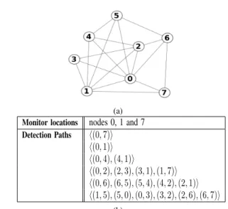
(a) Monitor locations nodes 0, 1 and 7
Detection Paths ⟨(0, 7)⟩ ⟨(0, 1)⟩ ⟨(0, 4), (4, 1)⟩ ⟨(0, 2), (2, 3), (3, 1), (1, 7)⟩ ⟨(0, 6), (6, 5), (5, 4), (4, 2), (2, 1)⟩ ⟨(1, 5), (5, 0), (0, 3), (3, 2), (2, 6), (6, 7)⟩ (b)
Fig. 1: Illustrative network topology, (a), and an associated detection solution, (b).
Theorem 2 states that the set of suspect links returned at the end of the detection phase whenever an anomaly on link e occurs is ∩p∈De+p− ∪p∈De−p. Therefore, instead of computing monitors that are to be activated and paths that are to be monitored during the localization phase whenever an anomaly is detected, we propose to perform these compu-tations for all potential anomalies only once offline. Having a set of detection paths that cover all links of the network, we infer the set of suspect links for all potential anomalies as described in Theorem 2. Then, a single anomaly scenario is
TABLE I: Sets of suspect links for all potential anomalies Anomalous link Set of suspect links
(0, 1) {(0, 1)} (0, 2) {(0, 2), (1, 3), (1, 7)} (1, 2) {(0, 6), (5, 6), (4, 5), (2, 4), (1, 2)} (0, 3) {(1, 5), (0, 5), (0, 3), (2, 6), (6, 7)} (1, 3) {(0, 2), (1, 3), (1, 7)} (2, 3) {(2, 3)} (0, 4) {(0, 4), (1, 4)} (1, 4) {(0, 4), (1, 4)} (2, 4) {(0, 6), (5, 6), (4, 5), (2, 4), (1, 2)} (0, 5) {(1, 5), (0, 5), (0, 3), (2, 6), (6, 7)} (1, 5) {(1, 5), (0, 5), (0, 3), (2, 6), (6, 7)} (4, 5) {(0, 6), (5, 6), (4, 5), (2, 4), (1, 2)} (0, 6) {(0, 6), (5, 6), (4, 5), (2, 4), (1, 2)} (2, 6) {(1, 5), (0, 5), (0, 3), (2, 6), (6, 7)} (5, 6) {(0, 6), (5, 6), (4, 5), (2, 4), (1, 2)} (0, 7) {(0, 7)} (1, 7) {(0, 2), (1, 3), (1, 7)} (6, 7) {(1, 5), (0, 5), (0, 3), (2, 6), (6, 7)} TABLE II: Anomaly scenarios Anomaly scenario Set of suspect links
a1 Sa1 ={(0, 2), (1, 3), (1, 7)}
a2 Sa2 ={(0, 6), (5, 6), (4, 5), (2, 4), (1, 2)} a3 Sa3 ={(1, 5), (0, 5), (0, 3), (2, 6), (6, 7)} a4 Sa1 ={(0, 4), (1, 4)}
created for all links that have the same set of suspect links, i.e., an anomaly scenario is created for each distinct set of suspect links. Let us denote by A the set of all anomaly scenarios, and let Sa denotes the set of suspect links associated to the anomaly scenario a ∈ A. Let dS = {Sa,∀a ∈ A}. dS have the following properties.
Corollary 4: ∪e∈ES(e) = ∪S(i)∈dSS(i) = E
Corollary 5: ∑S(i)∈dS| S(i) | = | E |
Clearly, an upper bound of the number of anomaly sce-narios, whatever the topology of network and whatever the detection solution, is the number of the network links. It is easy to show that when this bound is reached, the set of suspect links for an anomaly on link e, ∀e ∈ E, is reduced to the link e. In such case, the localization of all potential anomalies is immediate from the detection information. According to Corollary 2, we need to deploy monitors that enable the monitoring of a set of paths distinguishing links of each anomaly scenario pairwise in order to ensure the localization of all potential anomalies.
To illustrate, consider the sample network topology depicted in Figure 1(a). An associated anomaly detection solution that covers all links of the network is depicted in Figure 1(b). We use Theorem 2 to compute the set of suspect links for all potential anomalies. The result is depicted in Table I. The sets of suspect links associated to link (2, 3) and link (0, 7) are unitary. When an anomaly occurs on one of these two links, there is no need to trigger the localization phase because the anomalous link is immediately pinpointed by intersecting the detection paths that exhibit the anomaly. Furthermore, four non-unitary anomaly scenarios (a1, a2, a3, a4) are created for this topology (see table II). These are the four distinct non-unitary sets of suspect links.
Let AllP airs denotes the number of all the network link pairs. Clearly, AllP airs = (| E | (| E | −1))/2. Let dP airs
denotes the number of pair of links that need be distinguishable for localizing any potential link-level anomaly.
Corollary 6: dP airs = AllP airs - ∑
S(i),S(j)∈dS:i<j
| S(i) || S(j) | Corollary 6 confirms that we do not need to distinguish between all the network link pairs unless the number of detection paths equals 1, which is very unlikely.
The proofs of Corollary 4, Corollary 5 and Corollary 6 are described in Appendix A.
V. ANOMALY LOCALIZATION COST
Consider a set of candidate monitor locations,M, a set of network paths that are candidate to be monitored, P, and a set of anomaly scenarios A. The anomaly localization cost includes two costs:
• Monitor cost: it includes the effective cost of acquiring hardware and software monitoring devices and the cost of their maintenance. In addition, it includes the cost of communications between the monitors and the NOC. For instance, the cost of communications between a monitor and the NOC can be expressed as a function of the number of routing hops that separates them. Let us denote by Cn the cost of deploying a monitor on node n. Let Yn be a binary variable that indicates whether node n is selected to hold a monitoring device. The monitor cost can be expressed as
follows: ∑
n∈M
CnYn (1)
• Probe cost: it expresses the overhead of monitoring flows on the underlying network. Measurements of links that do not provide localization information should be avoided in order to minimize the monitoring overhead. Clearly, measuring links that do not belong to the set of suspect links of an anomaly scenario does not provide any ex-tra localization information. Furthermore, measurement of links that belong to the set of suspect links might be useless. Revisit Figure 1 and table I to illustrate. Con-sider an anomaly on link (6, 7). The associated set of sus-pect links is Sa3 = {(1, 5), (0, 5), (0, 3), (2, 6), (6, 7)}. Con-sider now the set of localization paths{p1:⟨(1, 5)(5, 6)(2, 6)⟩; p2:⟨(1, 5)(0, 5)(0, 2)⟩; p3:⟨(1, 7)(6, 7)(2, 6)⟩} that distinguishes between all the links ofSa3 pairwise. Path p1dividesSa3into two subsets:S1
a3{(1, 5), (2, 6)}andS 2
a3{(0, 5), (0, 3), (6, 7)}. p1 distinguishes each link of S1
a3 from each link of S 2 a3. Link
(5, 6)that is traversed by p1does not belong toSa3, and there-fore, it does not provide any localization information. Path p2 dividesSa13 into two subsets: S
11
a3{(1, 5)}andS 12
a3{(2, 6)}, and divides S2
a3 into two subsets: S 21
a3{(0, 5), (6, 7)} and S22
a3{(0, 3)}. Finally, p3distinguishes between(0, 5)and(6, 7). However, it crosses (2, 6)that is already distinguished from all the other suspect links. Thus, measuring (2, 6) by p3 does not provide extra localization information, although it belongs to Sa3.
Let us denote by Cethe cost of measuring link e. Ceshould be proportional to the load of link e, in order to avoid multiple measurements of the most overloaded links of the network.
Consider an anomaly scenario a∈ A. Let us denote by Sa the set of suspect links associated to the anomaly scenario a. Let Xpa be a binary variable that specifies whether path p is part of the localization solution of a. Let δpe be a binary input parameter that indicates whether path p crosses link e. The probe cost of the localization solution of a reads as
follows: ∑
e∈E,p∈P′
CeδpeXpa (2)
VI. ILP FORMULATION
The objective of the ILP is to find a localization solution for each anomaly scenario inA such that the anomaly localization cost is minimized. Let δpnbe a binary parameter that indicates whether node n is an end-node of path p. For simplicity of notation, we define the following sets:
• δPE ={δpe; p∈ P, e ∈ E}
• δPM={δpn; p∈ P, n ∈ M}
• CM={Cn; n∈ M} • CE ={Ce; e∈ E}
Let α be the weight associated to the monitor cost, and let β be the weight associated to the probe cost. α, β ∈ R. The input into the ILP is an instance of the graph G =
(E, M, P, A, δPE, δPM, CE, CM, α, β). The objective
func-tion minimizes the sum of the monitor cost and the probe cost. It reads as follows:
α ∑ n∈M CnYn+ β ∑ a∈A,e∈E,p∈P CeδpeXpa (3)
The ILP is subject to two constraints. The first constraint ensures that either end node of each selected monitoring paths is selected as monitor location. It reads as follows:
Yn ≥ δpnXpa; ∀n ∈ M, ∀p ∈ P, ∀a ∈ A (4)
The second constraint ensures that the suspect links asso-ciated to each anomaly scenario are distinguishable pairwise. To this end, according to Theorem 2, the constraint ensures that for each anomaly scenario a and for each pair of suspect links (e1, e2) : e1, e2∈ Sa there exists at least one monitoring path that crosses either e1 or e2, but not both. This constraint reads as follows:
∑
p∈P(δpe1+ δpe2− 2δpe1δpe2)Xpa> 0; ∀a ∈ A; ∀e1, e2∈ Sa (5)
We show that the above inequality is sufficient to distinguish between all the link pairs of each anomaly scenario using the argument of the following theorem.
Theorem 3: Let P1be the subset of paths ofP that cross
ei-ther e1or e2, but not both.∑p∈P(δpe1+ δpe2− 2δpe1δpe2) =| P1|.
Proof: Refer to Appendix B.
Corollary 7: If ∑p∈P(δpe1+ δpe2− 2δpe1δpe2)Xpa> 0,
then there exists at least one path inP that crosses either e1
or e2 but not both, then there exists at least one path inP
that distinguishes between e1 and e2.
VII. THEANOMALYLOCALIZATIONPROBLEM IS
N P-HARD
Theorem 4: The anomaly localization problem presented in
the previous section isN P-Hard.
Proof: Our formulation of the anomaly localization prob-lem can be reduced from the N P-Hard facility location problem.
Facility location problem[17]: consider a set of potential facility locationsF, and a set of clients D. Opening a facility at location i incurs a non-negative cost that is equal to fi. The cost of servicing client j∈ D by a facility installed at location
i ∈ F is dij. The problem is to find an assignment of each
client to exactly one facility such that the sum of the facility opening costs and the service costs is minimized.
We denote by f the set of facility opening costs, f = {fi, i ∈ F}, and by d the set of service costs, d =
{dij; i ∈ F, j ∈ D}. Given an instance I = (D, F, f, d)
of the facility location problem, we produce an instance
R(I) = (E, M, P, A, δPE, δPM, CE, CM, α, β) of the
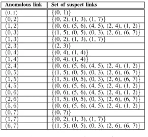
local-ization problem as follows. For each client j∈ D, we create: • Three nodes labeled by nj1, nj2, and nj3.
• One link connecting nj1 to nj2, labeled by ej1. • One link connecting nj2 to nj3, labeled by ej2. • An anomaly scenario aj such that Saj = {ej1, ej2}. For each facility location i ∈ F, we create two nodes labeled by mi1 and mi2. For each i ∈ F and for each
j ∈ D, we create one link connecting mi1 to nj1, labeled
by e1ij, and one link connecting mi2 to nj2, labeled by e2ij. We obtain a graphG = (E, N ), where N = {nik; i∈ D, k ∈ [1; 3]} ∪ {mjk; i∈ F, k ∈ [1; 2]}, and E = {ejk; j∈ D, k ∈ [1; 3]}∪{ek
ij; i∈ F, j ∈ D, k ∈ [1; 2]}. An example of a graph
constructed out of a facility location instance with four facility locations and four clients is shown in Figure 2.
Fig. 2: Example of a graph constructed out of a facility location instance with four facility locations and four clients
The candidate monitor location set is M = {mjk; i ∈ F, k ∈ [1; 2]}. The set of anomaly scenarios is A =
{aj; j ∈ D}. The set of candidate localization paths is
P = {pij; i ∈ F, j ∈ D}, where pij is the non-looping
path between mi1 and mi2 that crosses the links e1ij, ej1 and e2ij. The monitor deployment costs are defined as follows:
Cmi1 = Cmi2 = fi/2. The link measurement costs are defined
as follows: Cei1 = Cei2 = 0, Ce1ij = Ce2ij = dij/2. The remaining input parameters can be inferred easily fromG, M, A and P as follows:
• δajej′ k= { 1 if j = j′ 0 otherwise ; ∀j, j ′ ∈ D, k ∈ [1; 2] • δa jekij = 0; ∀i ∈ F, j ∈ D, k ∈ [1; 2] • δpijmi′ k = { 1 if i = i′ 0 otherwise ; ∀i, i ′ ∈ F, k ∈ [1; 2] • δpijej1= δpije1
ij = δpije2ij = 1; ∀i ∈ F, j ∈ D
• δpijej2= 0; ∀i ∈ F, j ∈ D
• α = β = 1
It can be easily shown that the time complexity of the above reduction is O(| F | × | D |), and therefore, it can be carried out in polynomial-time. In the sequel, we show that there is an optimal solution to the Instance I of the facility location problem if and only of there is an optimal solution to the instance R(I) of our anomaly localization problem.
Let us start by demonstrating that if there is an optimal solution to the facility location instance, then there is a feasible solution to the anomaly localization instance. Let the facility location solution assign each client j to a facility installed at location i. Consider the anomaly localization solution that selects for each anomaly scenario aj the path pij and the monitor locations mi1 and mi2. Then, let us fix an anomaly scenario aj. By construction, path pij crosses three links that are ej1and e1ij and e
2
ij. It follows, according to Theorem 1, that pij distinguishes between ej1 and ej2. Constraint (4) states that if pij is selected to be monitored, then, its end nodes must be selected to hold monitoring devices. Thus, the solution that selects for each anomaly scenario aj the path pij to be monitored, and its end nodes, mi1 and mi2, as monitor locations is a feasible solution to the anomaly localization instance.
Conversely, we demonstrate that if there is an optimal solution to the anomaly localization instance, then there is a feasible solution to the facility location instance. An optimal solution to the facility location problem selects exactly one path for each anomaly scenario. This is because, by construction, for each anomaly scenario ai ∈ A | Sai |= 2. Thus, monitoring one path that crosses exactly one of the two links is sufficient to distinguish between them. Let the optimal anomaly localization solution selects for each anomaly scenario aj the path pij, and naturally, the monitor locations mi1 and mi2. Trivially, the solution that assigns to each client j ∈ D the facility installed at location i is a feasible solution to the facility location instance.
We now prove that the constructed anomaly localization solution has the same cost as its corresponding optimal facility location solution (the proof holds in the converse case). Let Wi be a binary variable that indicates whether a facility is installed at location i, and let Zij be a binary variable that indicates whether client j is serviced by a facility installed at location i. Using the arguments that Zij = Xpijaj and Wi = Ymi1 = Ymi2
3, we show that the cost of the localization solution, denoted by
Cost(SR(I)), is equal to the cost of its corresponding
3Recall that X
pais a binary variable that indicates whether path p is part
of the localization solution of the anomaly scenario a, and Yn is a binary
variable that indicates whether node n is selected as a monitor location
facility location solution, denoted by Cost(SI), as follows:
Cost(SR(I)) = α ∑ mik∈M CmikYmik+ β ∑ aj∈A,e∈E,pij∈P CeXpijaj = ∑ mik∈M CmikYmik+ ∑ aj∈A,pij∈P (Ce1 ij+ Ce 2 ij)Xpijaj = ∑ mi1∈M fiYmi1+ ∑ aj∈A,pij∈P dijXpijaj =∑ i∈F fiWi+ ∑ j∈D,i∈F dijZij = Cost(SI)
Now, we show that the solution to the anomaly localization instance, denoted by SR(I), that is constructed out of an optimal solution to the facility location instance, denoted by SI∗, is optimal. Assume to the contrary that SR(I) is not optimal. Let SR(I)′∗ be an optimal solution to the anomaly lo-calization instance, and let SI′ be the facility location solution constructed out of SR(I)′∗ . We have Cost(SI∗) = Cost(SR(I)) <
Cost(S′R(I)∗ ) = Cost(S
′
I), leading to a contradiction. Using the
same arguments, we can show that the solution to the facility location instance constructed out of an optimal solution to the anomaly localization instance is optimal.
VIII. HEURISTIC SOLUTION
In this section, we provide a monitor location and path selection algorithm for localizing single link-level anomalies. The inputs of the algorithm are a network graphG = (N , E), a set of anomaly scenarios A, a set of candidate monitor locations M, the costs of deploying monitoring devices on the network nodes CM = {Cn; n ∈ M}, and the costs of monitoring the network links CE = {Ce; e ∈ E}. The outputs are a set of monitor locations, SMa, and a set of monitoring paths,SPa, that can distinguish between all links of Sa pairwise, for each a∈ A.
Similarly to the ILP, the heuristic solution aims at min-imizing the infrastructure cost, the communication cost and the probe cost jointly. To this end, we use a nested greedy approach that selects monitor locations jointly with monitoring paths. Algorithm 1 describes the pseudo-code. ProbeCost(p, CE) is a function that returns the probe cost incurred by monitoring path p. This cost is computed as described in section V. ms stores the best current candidate monitor location. SM stores the monitor locations selected at the previous iterations. Pcostmin stores the current lowest probe cost, and lcmax stores the current largest localization capacity, i.e., the number of link pairs that can be distinguished by monitors inSM ∪ {ms}. CP stores paths selected by the current best solution. In the sequel, we define the criteria of monitor location selection and monitoring path selection.
A detailed description of how monitor locations and monitoring paths are selected, and how candidate localization paths are computed is provided in the following subsections. A. Selection of monitor locations
The algorithm starts by selecting one candidate monitor location randomly. Alternatively, the candidate monitor loca-tion with the smallest monitor cost (sum of the infrastructure cost and the communication cost) can be selected. However, we advocate random selection for two reasons. The first is
Algorithm 1: Monitor location and path selection algo-rithm for single anomaly localization
1 nbPairs =
∑
a∈A |S∑a|−1
k=1
k; Pcostmin← INT MAX; lcmax
← 0; CP ← ∅;
2 SM ← {selectRandomElement(M)}; Remove the
selected monitor location fromM;
3 while (M ̸= ∅) do
4 Reset ms← Null;
5 foreach (m∈ M) do
6 if (( lcmax = nbP airsand βPcostmin ≤ αCm))
then Jump to line 5;
7 Reset lc← 0; Reset Pcost ← 0; 8 for (a∈ A) do 9 ClearPa; ClearMa; 10 j← 1; s(0)← 1; S (0)1 a ← Sa; 11 while (s(j)> 0) do 12 Sa(j)← {Sa(j)1, ...Sa(j)k,Sa(j)k+1...,S (j)s(j) a }; 13 pa(j)← CandidatePathSelection(m, SM, G, Sa(j),CP); lc +=∑1≤k≤s (j)lc(pa(j),S (j)k a );
14 Pcost += P robeCost(pa(j), CE);
15 l← 1; 16 for (1≤ k ≤ s(j)) do 17 if (| pa(j)∩ Sa(j)k|> 1) then S(j+1)l a ← pa(j)∩ S (j)k a ; l← l + 1; 18 if (| Sa(j)k− {pa(j)∩ S (j)k a } |> 1) then S(j+1)l+1 a =Sa(j)k− {pa(j)∩ S (j)k a }; l← l + 1; 19 end 20 s(j)← l − 1;
21 if (lcmax = nbP airsand (αCm+ β(PCost
+
s(j+1)∑ l=1
ThMinPCost(Sa(j+1)l) +
∑
a′∈A,a′>aThMinPCost(Sa′)) ≥
22 αCms+ βPcostmin)) then
23 /*Stop the exploration of the current
candidate monitor location*/
24 Jump to line 5;
25 end
26 Add the end nodes of pa(j)toMa;
27 Add pa(j)to Pa;
28 j← j + 1;
29 end
30 end
31 if (lc > lcmaxor (lc = lcmaxand
αCm+ βP cost < αCms+ βPcostmin)) then 32 ms← m; lcmax← lc;
33 Pcostmin← P Cost; SPa← Pa;SMa← Ma;
34 end
35
36 end
37 if (ms= N ull) then return ({SPa,SMa}; ∀a ∈ A)
38 UpdateCP ←
∪
a∈A
SPa;
39 Add ms toSM; Remove ms fromM;
40 end
41 return({SPa,SMa; ∀a ∈ A});
that the monitor location with the smallest monitor cost does not necessarily incur the smallest probe cost. The second is that selecting the starting point randomly enlarges the space
of explored solutions over multiple runs of the algorithm. Monitor locations are, then, added to the solution greedily until all link pairs of all the anomaly scenarios are distinguished. At each greedy iteration (lines 5-36), all the remaining candidate monitor locations are explored. Let us fix a candidate monitor location m. A set of monitoring paths whose end nodes are
in SM ∪ {m} is selected greedily (lines 7-35). The path
selection procedure is described in details in section VIII-B. The candidate monitor location whose associated monitoring paths can distinguish between the largest number of link pairs over all the anomaly scenarios is selected (line 31). In case of a tie, a monitor location that incurs the smallest localization cost (α× monitor cost + β × probe cost, where the probe cost is the summation of the probe costs of the associated monitoring paths) is selected.
When a solution that distinguishes between all the link pairs of all the anomaly scenarios is found, the algorithm continues the exploration of the remaining candidate monitor locations, if any, towards reducing the probe cost. However, a filter is applied on these locations before exploring them (line 6). Only candidate locations whose monitor cost is smaller than the probe cost of the current best solution are explored. Clearly, the localization cost of any solution that selects a monitor location not satisfying this filter would be larger than the localization cost of the current best solution. The algorithm ends when the set of candidate monitor locations gets empty, i.e., all candidate monitor locations have been selected, or when remaining candidate monitor locations can neither improve the localization capacity nor the probe cost of the current best solution.
B. Selection of localization paths
Given a candidate monitor location m and a set of already selected monitor locationsSM, the procedure of selecting an associated set of monitoring paths, (lines 7-35), is as follows. Let us fix an anomaly scenario a. A set of monitoring paths that maximizes the number of distinguished pair of links of Sa while minimizing the probe cost is selected greedily as follows. First, one path that can distinguish between the largest number of link pairs ofSais selected. We refer to the number of pair of links of a set of suspect links Sa that can be distinguished by a path p as the localization capacity of p with respect toSa, denoted by lc(p,Sa). It can be easily shown that:
lc(p,Sa) =| p ∩ Sa| (| Sa|− | p ∩ Sa|) (6)
In case of a tie, a path that minimizes the probe cost is selected. The algorithm used for computing the candidate monitoring path is described in section VIII-C. Let pa(1) be the selected path. Two subsets of suspect links are generated:
S(1)1
a =Sa∩ pa(1)andS (1)2
a =Sa− {Sa∩ pa(1)}. According
to Theorem 1, pa(1) distinguishes between every pair of links (e1, e2) such that e1∈ S
(1)1
a and e2∈ S (1)2
a . At the next step, we need to distinguish between the links of Sa(1)1 pairwise and between the links of Sa(1)2 pairwise. Hence, a path that maximizes lc(p,Sa(1)1) + lc(p,S
(1)1
a ) is selected. Ties are broken by selecting a path that minimizes the probe cost.
Let pa(j) be the monitoring path selected at step (j). Let s(j−1) be the number of non-unitary subsets of suspect links generated at step (j − 1). pa(j) is selected such that ∑
1≤k≤s(j−1)lc(p, S
(j−1)k
a ) is maximized. In case of a tie, a path that minimizes the probe cost is selected. For each
S(j−1)k
a ,1≤ k ≤ s(j−1), two subsets of suspect links are
gen-erated:Sa(j−1)k∩ pa(j) andS (j−1)k
a − {S
(j−1)k
a ∩ pa(j)}. Each
link of the former subset is distinguished from each link of the latter subset. Only non-unitary subsets, whose links need to be distinguished from each other, are considered at the next step. This greedy process is re-iterated until all the generated subsets of suspect links are unitary or until no candidate localization path can distinguish between the pair of links of non-unitary subsets. For each selected path pa(j), the localization capacity of m is incremented by lc(pa(j),S
(j)
a ) (line 13), and its probe cost is incremented by probeCost(pa(j), CE) (line 14). The above procedure is applied on the all the anomaly scenarios
in A. Then, the localization capacity and the probe cost of
m are evaluated (line 31). If the localization capacity of m is greater than lcmax, or if the localization capacity of m equals lcmax and its probe cost is less than Pcostmin; then lcmax is set equal to the localization capacity of m, Pcostmin is set equal to the probe cost of m and ms is set equal to m.
Furthermore, using the argument of the following theorem, we can compute a lower bound of the probe cost of the explored monitor location at any step in the path selection procedure.
Theorem 5: The theoretical minimal probe cost relative to
a set of suspect links S denoted by T hMinP cost(S) reads
as follows:
T hM inP cost(S) =∑
e∈S
Ce− max
e∈SCe (7)
Proof: Refer to Appendix C.
The lower bound of the probe cost of a candidate monitor location after path pa(j) is added to the set of its associated monitoring paths reads as follows:
P cost + s(j) ∑ k=1 T hM inP cost(S(j)k a ) + ∑ a′∈A,a′>a T hM inP cost(Sa′) (8)
where P cost is the summation of the probe costs of the already selected paths.
When the algorithm finds a solution that can distinguish between all link pairs of all the anomaly scenarios, it continues exploring the remaining candidate monitor locations that sat-isfy the monitor cost filter (line 6) towards reducing the probe cost. Using (8), we propose an optimization of the exploration process of these candidate monitor locations. The idea is to update the lower bound of the probe cost of the explored monitor location whenever a monitoring path is selected, and to infer a lower bound of the localization cost (line 21). The exploration of the considered candidate monitor location is abandoned if, at any step of the path selection procedure, the calculated lower bound of the localization cost dominates the localization cost of the current best solution.
Procedure 2: candidatePathSelection(m,SM, G, Sa(j), CP) 1 pc← newPath(); 2 limin←∑S(j)k a ∈S(j)a | S (j)k
a | /2 − 1; Pcostmin←∑e∈ECe;
3 foreach q∈ CP do 4 li =∑ S(j)k a ∈Sa(j)| S (j)k a | /2− | S (j)k a ∩ q |;
5 if (li < liminor (li = liminand
probeCost(pc, CE) < Pcmin)) then
6 limin= li; Pcmin= probeCost(pc, CE); ps= q;
7 end
8 end
9 add-node-to-path(m, pc);
10 depthFirst (m, pc){
11 foreach (n∈ children(m, G) and (m, n) /∈ pc) do
12 add-node-to-path(n, pc); 13 li(pc,Sa(j)) = ∑ S(j)k a ∈Sa(j)|| S (j)k a | /2− | Sa(j)k∩ pc||; 14 if (n∈ SM) then 15 if (li(pc,S (j) a ) < liminor (li(pc,S (j) a ) = limin
and probeCost(pc, CE) <= Pcmin)) then
16 ps← pc; limin← li(pc,S
(j)
a );
Pcmin= probeCost(pc, CE);
17 if (limin= 0 and Pcmin= 0) then
18 /*Stop the algorithm*/ Jump to line 31;
19 end
20 end
21 else
22 if
((limin= 0and (probeCost(pc, CE)+li(pc,Sa(j))−
limin>= Pcminor∃ Sa(j)k∈ Sa(j)such that
23 | Sa(j)k∩ pc|>| S (j)k a | /2)) or (li(pc,S (j) a ) > limin and∀ S (j)k a ∈ S (j) a | S (j)k a ∩ pc|>| S (j)k a | /2)) then
24 do not explore the descendants of n;
25 else
26 Recursively call depthFirst (n, pc);
27 end
28 end
29 end
30 } 31 return ps;
C. Candidate path selection algorithm
This section describes the procedure candidatePathSelec-tion called by Algorithm 1 at line 13. The inputs into this procedure are the network graph, the currently explored monitor location m, the subsets of suspect links generated at the current step of the path selection procedure Sa(j) =
{S(j)1
a , ... Sa(j)k,Sa(j)k+1 ...,S
(j)s(j)
a }, the set of the already
selected monitor locations SM, and the set of monitoring paths selected by the current best solution CP. The output is one monitoring path, whose end nodes are inSM ∪ {m}, that maximizes the localization capacity while minimizing the probe cost.
The main difficulty of this procedure is the computation of the set of candidate paths. Generally, the smaller the set of candidate paths is, the worst the quality of the heuristic is. This is because good paths might be missed when reducing the number of candidate paths. However, this reduction is
imper-ative to ensure the scalability of the heuristic. The procedure candidatePathSelection implements an algorithm for candidate localization path computation. The algorithm considers all the network paths whose end nodes belong to {m} × SM as candidate to be monitored. However, computing this set of paths is computationally expensive, because it requires exploring all the network graph. Moreover, since Algorithm 1 explores all remaining candidate monitor locations at each iteration, the graph would be explored multiple times; which makes the heuristic non-scalable and non-practical for dense networks. An alternative solution is to compute and store all paths traveling between all candidate monitor locations offline, thereby reducing the number of times the network graph is explored to one. Clearly, this solution is impractical due to memory issues. We conclude, based on the above discussion, that our candidate path computation algorithm must minimize the number of paths that are to be explored, while guaranteeing that good candidate paths are not missed. To this end, we make use of the argument of the following theorem:
Theorem 6: let lc(Sa(j), p) = ∑ S(j)k a ∈S(j)a lc(S (j)k a , p) be the localization
capacity of p with respect to S(j). We have,
max p∈P lc(S (j) a , p) = min p∈P ∑ S(j)k a ∈S (j) a || S(j)k a | /2− | S (j)k a ∩ p || (9)
Proof: Refer to Appendix D. We refer to ∑S(j)k
a ∈Sa(j) || S (j)k
a | /2− | Sa(j)k ∩ p ||
as the localization indicator of path p with respect to Sa(j), and we denote it by li(p,Sa(j)). According to Theorem 6, the smaller li(p,Sa(j)) is, the higher the localization capacity of p with respect to Sa(j) is. The localization indicator is used along with the probe cost to avoid exploring all the network graph, while guaranteeing that good candidate paths are not missed. Procedure 2 provides an overview of the pseudo-code. ps stores the current best candidate path, limin stores the localization indicator of ps, and Pcmin stores its probe cost. ps, limin and Pcmin are initialized to N ull, ∑ S(j)k a ∈S (j) a | S (j)k a | /2 − 1 and ∑ e∈ECe, respectively. Note that the least upper bound of the localization indicator is ∑S(j)k
a ∈S(j)a | S (j)k
a | /2, which corresponds to a path that
does not provide any localization information (i.e., ∀Sa(j)k ∈
S(j)
a ,Sa(j)k∩ p = ∅ or ∃Sa(j)k ∈ Sa(j) such that p = Sa(j)k)4;
whereas the least upper bound of the probe cost is∑e∈ECe, which corresponds to a path that crosses all the network nodes and does not provide any localization information. However,
if CP is not empty, then ps is set equal to the best path
in CP, i.e., the path that maximizes the localization capacity
(in case of a tie, a path that minimizes the probe cost); and liminand Pcminare initialized to the localization capacity and the probe cost of that path, respectively. The rational behind considering paths inCP is to avoid re-exploring all candidate paths traveling between the already selected monitors.
4By construction,∩
kS
(j)k
a =∅
The network graph is, then, explored in depth-first order starting from the candidate monitor location m. It is worth noting that we believe that a breadth-first search can find can-didate paths faster. However, the depth-first search approach requires much less memory.
We now introduce the optimizations made to avoid ex-ploring all the network graph, which speeds up the search and ensures the scalability of the algorithm. Let n be the currently explored node and pc the current path to that node. ps , limin and Pcmin are set equal to pc, li(pc,S
(j) a ), and
probeCost(pc, CE), respectively, if the following condition is
true:
n∈ SM and(li(pc,Sa(j)) < liminor (li(pc,Sa(j)) = limin and
probeCost(pc, CE) < Pcmin)) (10)
The above condition implies that the path selection criterion is the minimization of the localization indicator, which is equivalent to the maximization to the localization capacity, and that ties are broken by minimizing the probe cost. Moreover, it ensures that the end nodes of the selected path are in SM ∪ {m}.
Now, the most important feature of the algorithm is that it is able, using Theorem (6), to decide whether all paths having a given prefix are not good. A good path is a path that dominates the current best path, i.e., a path that satisfies Condition (10). In fact, all paths having as prefix the current path pc are undoubtedly inefficient if one of the following conditions is true:
limin= 0 and∃ Sa(j)k∈ Sa(j)such that| Sa(j)k∩ pc|>| Sa(j)k| /2 (11)
limin= 0 and∀Sa(j)k∈ S (j) a | S (j)k a ∩pc |≤| Sa(j)k| /2 and probeCost(pc, CE) + min e∈E Celi(pc,S (j) a )≥ Pcmin (12)
li(pc,Sa(j)) > liminand∀Sa(j)k∈ Sa(j)| Sa(j)k∩ pc|≥| Sa(j)k| /2 (13)
Whenever a node that is not inSM is explored, the current path to that node is examined. If it satisfies one of the above conditions, then the descendant nodes of the current node will not be explored, i.e., all paths having as prefix the current path will be discarded without exploring their suffixes. This achieves great savings in terms of the number of explored paths and in terms of time. The accuracy of conditions (11), (12) and (13) is demonstrated in Appendix E.
IX. PERFORMANCEEVALUATION
Extensive simulations are conducted on network topologies built using the BRITE generator [18] (Waxman model [19]:
α = β = 0.4, random node placement 5). We use Cplex11.2
[20] to solve ILPs and we implement our algorithms using C++. All the numerical results presented in this section are the mean over 30 simulations on random simulations. Our exper-iments indicate that the results are almost the same for larger number of simulations. Table III depicts a summary of the topologies considered. Our localization scheme takes as input 5These parameters are not to be confused with the monitor cost weight (α) and the probe cost weight (β) introduced in Section VI. Their values equal the values used by Waxman to generate network topologies [19].
any detection solution that covers all links of the network. For small topologies, i.e., TOP(8, 18), optimal detection solutions are computed using the detection scheme proposed in [13]; whereas the anomaly detection heuristic proposed in [14] is used to compute detection solutions for larger topologies. Note that the anomaly detection problem is N P-Hard, therefore, optimal detection solutions could not be computed for large topologies.
TABLE III: Summary of the topologies considered in the evaluation
Topology Nb. of nodes Nb. of links
TOP(8, 18) 8 18
TOP(10, 31) 10 31
TOP(12, 41) 12 41
TOP(15, 59) 15 59
TOP(20, 80) 20 80
The evaluations are performed on a PC equipped with a 2,992.47 MHz Intel(R) Core(TM)2 Duo processor and 3.9 GB of RAM. We assume that every nodes of the network is candidate to support a monitoring device and all paths of the networks are candidate to be monitored. We set Cn = Ce=
1,∀n ∈ N and ∀e ∈ E.
A. Comparing our Anomaly Localization Scheme with Exist-ing Schemes
We compare our anomaly localization scheme with an hy-brid anomaly localization scheme that combines the strengths of the schemes proposed in [1] and [2]. As proposed in [2], a set of paths that distinguishes only between the suspect links is monitored during the localization phase. However, to guarantee that all potential anomalies can be localized uniquely, a set of monitors that can distinguish between all pairs of the network links is deployed [1]. Such a scheme can be formulated as two ILPs. The first ILP computes a minimal subset of monitor locations that enables the localization of all potential anomalies. This ILP is run only once offline. It reads as follows:
Minimize∑n∈MYn Subject to:
∑
p∈P(δpe1+ δpe2− 2δpe1δpe2)Zp> 0;∀e1, e2∈ E; ∀p ∈ P
δpnYn≥ Zp; ∀p ∈ P, ∀n ∈ N
The second ILP is run whenever an anomaly is detected. The input is the set of monitor locations selected by the first ILP, M′, and a set of suspect linksS. The output is a minimal set of monitoring paths that can distinguish between the suspect links pairwise. This ILP reads as follows:
Minimize∑p∈PZp Subject to:
∑
p∈P(δpe1+ δpe2− 2δpe1δpe2)Zp> 0;∀e1, e2∈ S; ∀p ∈ P
Zp≤ δpnYn; ∀p ∈ P, ∀n ∈ M
′
We refer to this hybrid anomaly localization scheme as HLS. Only small topologies for which the ILPs can deliver solutions in tractable time are considered. We set the weight associated to the probe cost β = 1, and we vary the weight associated to the monitor cost, α∈ [1, 2, 4] and α ≥ 6.
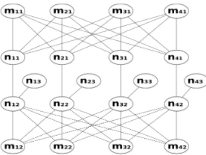
0 1 2 3 4 5 HLS _ = 1 _ = 2 _ = 4 _ >= 6
Avg. nb. of monitoring paths per anomaly
Fig. 3:Average number of monitoring paths per anomaly for TOP(8, 18). The first histogram to the left presents results for solutions computed using the hybrid localization scheme (HLS), and the other histograms present results for the solutions computed using our anomaly localization ILP with different values of α (β = 1).
We define three metrics for the comparison. The first metric is the time of computing the localization solution, i.e., monitors that are to be activated and paths that are to be monitored when an anomaly is detected. This metric reflects the speed of the localization scheme. The better is to avoid online computations, i.e., computations done upon detecting an anomaly, in order to shorten the localization delay.
TABLE IV: Average ILP computation time for TOP(8, 18) Hybrid scheme Our scheme Offline Computation Time 64.16 s 6.67 s Online Computation Time 25.7 10−3 s 0 s
Table IV depicts the online computation time and the offline computation time for the hybrid localization scheme and for our localization scheme. Intuitively, as shown in the table, the online computation time is zero for our localization scheme. This is because we compute full localization solutions for all potential anomalies offline. In contradiction, the hybrid scheme leaves the selection of monitoring paths upon detecting an anomaly, thereby achieving a non-negligible online computa-tion time. This time can be relatively high for large topologies where the number of candidate monitoring paths is large. For the offline computation time, the table shows that our scheme is about 10 times faster than the hybrid scheme, although, it computes full localization solutions for all potential anomalies. We explain this result by the fact that, unlike the hybrid scheme, our scheme does not distinguish between every pair of the network links.
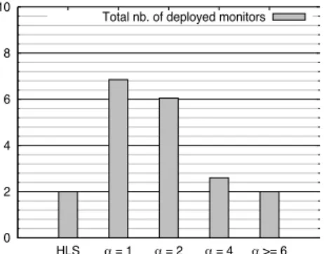
The second metric is the localization cost. Figure 4 plots the total number of deployed monitors (Figure 4c), the average number of monitors activated per anomaly (Figure 4b), and the average overhead (4a), i.e., the number of links monitored that provide no localization information, per anomaly for the hybrid localization scheme and for our localization scheme with different values of α. Three conclusions can be drawn from the numerical results. The first is that there is an interplay between the monitor location cost and the probe cost. The different results for the different values of α illustrate this conclusion. Indeed, the larger the value of α is, the fewer the number of monitors is and the larger the localization
0 1 2 3 4 5 6 7 8 9 10 HLS _ = 1 _ = 2 _ = 4 _ >= 6 Avg. overhead per anomaly
(a) Average overhead per anomaly
0 2 4 6 8 10 RProc(0.015%)RProc(0.03%)RProc(0.15%)RProc(0.3%)Procedure1 Avg. nb. of active monitors per anomaly
(b) Average nb. of monitors activated per anomaly
0 2 4 6 8 10 HLS _ = 1 _ = 2 _ = 4 _ >= 6 Total nb. of deployed monitors
(c) Total nb. of deployed monitors Fig. 4:Localization costs for TOP(8, 18)
overhead is. For instance, for α = 1, we have localization solutions with zero overhead and 7 monitors, i.e., 7 of the 8 nodes of the network hold monitoring devices. The second is that the existing localization scheme that deploys monitors offline and selects monitoring paths online does not take into consideration this interplay, and therefore, delivers sub-optimal localization solutions. Using the same number of monitors, for
α ≥ 6, our localization scheme can localize any potential
anomaly with about 65% less overhead than the existing localization scheme.
The third metric is the number of monitoring paths. Re-call that this is the path selection criterion for the existing localization scheme. We do not consider this criterion in our localization scheme for two reasons. The first is that, upon detecting an anomaly, the set of paths that distinguish between the suspect links are monitored simultaneously. Therefore, the minimization of the number of monitoring paths does not reduce the localization delay. The second reason is that this metric is tightly correlated to the number of monitors and the localization overhead. Indeed, if we relax the constraint on the localization overhead, this would allow long monitoring paths that cross a large number of links. Therefore, the number of monitoring paths that can distinguish between the suspect links would decrease. Similarly, if we relax the constraint on the number of monitors, we would deploy more monitors in the network, thus, the monitoring paths would get shorter. Therefore, the number of monitoring paths that can distinguish between the suspect links would increase. Figure 3 validates these claims. Hereby, we can observe that the larger α is, the more monitoring paths we have. Not surprisingly, for α≥ 6, our localization scheme monitors only 8% more paths than the hybrid localization scheme, while deploying the same number of monitors and incurring 65% less overhead.
B. Evaluating the Scalability and Quality of the Heuristic In this section, we evaluate the performance of our anomaly localization heuristic. We set α >> β. For each network topology, we run the heuristic n times, where n is the number of the network nodes. The first monitor location that is selected randomly must be different for each run. Then, we consider the solution with the smallest localization cost. For
TOP(8, 18), we compare the results obtained using the heuristic
with the results obtained using our anomaly localization ILP
(α≥ 6), and the results obtained using the hybrid localization
scheme. Furthermore, we evaluate the evolution of resource consumption and computation time with respect to the network size to evaluate the performance of the heuristic on larger topologies.
Table V depicts the heuristic computation time (this is the time of the n runs of the heuristic) and the average percentage of the network paths explored in one execution of Procedure 2 for all the topologies considered. For TOP(8, 18) the heuristic computation time is about 29.103 times faster than our ILP, and about 27.104 times faster than the hybrid localization scheme. Recall that all computations are done offline. For TOP(10, 31), TOP(12, 41) and TOP(15, 59)
the heuristic computation time is in the order of few seconds (< 25 s), while it was infeasible to obtain the ILP results for these topologies in tractable time. ForTOP(20, 80), whose number of paths is in the order of hundreds of billions, it was impossible to run the ILPs due to memory insufficiency. However, the heuristic succeeded to compute solutions in less than one hour for these topologies. This confirms the efficiency of our candidate path computation algorithm that minimizes the number of the networks paths that are to be explored. For instance, we found that only 0.007% of the network paths are explored in one execution of Procedure 2 for TOP(20, 80). TABLE V: Heuristic computation time (all computations are done offline) and percentage of paths explored in one execution of Proce-dure 2
Topology Heuristic computation % of paths explored in one
time execution of Procedure 2
TOP(8, 18) 0.00023 s 1.22%
TOP(10, 31) 0.08 s 0.21%
TOP(12, 41) 0.78 s 0.07%
TOP(15, 59) 24.11 s 0.02%
TOP(20, 80) 3525.52 s 0.007%
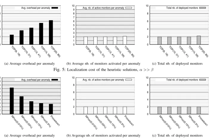
We now investigate the quality of the solutions delivered by the heuristic. Figure 5 plots the total number of monitors deployed (5c), the average number of monitors activated per anomaly (5b), and the average overhead per anomaly for the topologies considered in the evaluation5a.
First, we notice that two monitors are sufficient to localize all potential anomalies for all topologies, except TOP(20, 80)
0 2 4 6 8 10
TOP(8, 18) TOP(10, 31) TOP(12, 41) TOP(15, 59) TOP(20, 80) Avg. overhead per anomaly
(a) Average overhead per anomaly
0 1 2 3 4 5 6 7 8 9 10
TOP(8, 18) TOP(10, 31) TOP(12, 41) TOP(15, 59) TOP(20, 80) Avg. nb. of active monitors per anomaly
(b) Average nb. of monitors activated per anomaly
0 2 4 6 8 10
TOP(8, 18) TOP(10, 31) TOP(12, 41) TOP(15, 59) TOP(20, 80) Total nb. of deployed monitors
(c) Total nb. of deployed monitors Fig. 5:Localization cost of the heuristic solutions, α >> β
0 2 4 6 8 10 12 14 16 18 20 RProc(0.015%)RProc(0.03%)RProc(0.15%)RProc(0.3%)Procedure1 Avg. overhead per anomaly
(a) Average overhead per anomaly
0 2 4 6 8 10 RProc(0.015%)RProc(0.03%)RProc(0.15%)RProc(0.3%)Procedure1 Avg. nb. of active monitors per anomaly
(b) Avgerage nb. of monitors activated per anomaly
0 2 4 6 8 10 RProc(0.015%)RProc(0.03%)RProc(0.15%)RProc(0.3%)Procedure1 Total nb. of deployed monitors
(c) Total nb. of deployed monitors
Fig. 6: Impact of the number and the quality of candidate monitoring paths on the quality of the localization solution. RProc means random procedure (numerical results for TOP(15, 59))
for which the average number of monitors deployed and the average number of monitors activated per anomaly are slightly larger than two. This is expected, since we set α >> β, which means that the heuristic minimizes in priority the number of monitors that are to be deployed. A comparison of Figure 5 with Figure 4 shows that, for TOP(8, 18), the solutions computed using our ILP (α≥ 6) is very close to the solutions computed using the heuristic: the heuristic solution gnenerates about 9% more overhead, however, the two solutions deploy the same number of monitors and activate, in average, the same number of monitors when an anomaly occurs. This confirms that the candidate path computation algorithm that avoids exploring all paths of the network does not miss good paths. Moreover, the overhead of the heuristic solutions for TOP(10, 31),TOP(12, 41) andTOP(12, 59)is smaller than the overhead of the hybrid localization scheme solutions forTOP(8, 18). It is worth to recall that the hybrid localization solutions forTOP(8, 18) are exact solutions. This confirms that i) the heuristic succeeds to minimize the localization costs, i.e., the monitor cost and the probe cost, jointly; ii) the heuristic outperforms the hybrid localization scheme, since the former can localize anomalies in large topologies using less resources that those used by the latter to localize anomalies in smaller topologies. We finally evaluate the impact of the number and the quality of candidate monitoring paths on the quality of the localization solution. To this end, we compare the localization solutions obtained using the proposed heuristic, i.e., Algorithm
1 and Procedure 2, to the localization solutions obtained using Algorithm 1 and a procedure that computes candidate paths randomly (instead of Procedure 2). In the latter case, we variate the number of paths explored per one execution of the random candidate path computation procedure (0.015%, 0.03%, 0.15%, 0.3%). We report the results for TOP(15, 59)
when α >> β in Figure 6 (The results are essentially the same for the other topologies). Not surprisingly, Figure 6 shows that, when candidate paths are explored randomly, the larger the number of paths explored is the smaller the localization overhead is. Furthermore, it shows that the proposed heuristic achieves smaller overhead than the random approach, thought it explores more than 15 times less paths as shown in Table V. This validates our claim on the correlation between the number and quality of monitoring paths and the quality of the localization solution.
X. DISCUSSION
The anomaly localization solution must be updated when-ever the detection solution changes. Howwhen-ever, the detection solution changes in rare cases where a persistent anomaly makes a network link unavailable for a long period of time, or where the network topology is modified voluntary (e.g., add and/or removal of network equipments).
Usually, in the first case, the detection solution is updated partially. Only the detection paths that are affected by the anomaly are re-computed. The anomaly scenarios are updated accordingly, and the localization solution is re-computed,