CAPM, Components of Beta and the Cross Section of Expected Returns

Texte intégral

(1)2013s-09. CAPM, Components of Beta and the Cross Section of Expected Returns Tolga Cenesizoglu, Jonathan J. Reeves. Série Scientifique Scientific Series. Montréal Avril 2013. © 2013 Tolga Cenesizoglu, Jonathan J. Reeves. Tous droits réservés. All rights reserved. Reproduction partielle permise avec citation du document source, incluant la notice ©. Short sections may be quoted without explicit permission, if full credit, including © notice, is given to the source..

(2) CIRANO Le CIRANO est un organisme sans but lucratif constitué en vertu de la Loi des compagnies du Québec. Le financement de son infrastructure et de ses activités de recherche provient des cotisations de ses organisations-membres, d’une subvention d’infrastructure du Ministère du Développement économique et régional et de la Recherche, de même que des subventions et mandats obtenus par ses équipes de recherche. CIRANO is a private non-profit organization incorporated under the Québec Companies Act. Its infrastructure and research activities are funded through fees paid by member organizations, an infrastructure grant from the Ministère du Développement économique et régional et de la Recherche, and grants and research mandates obtained by its research teams. Les partenaires du CIRANO Partenaire majeur Ministère de l'Enseignement supérieur, de la Recherche, de la Science et de la Technologie Partenaires corporatifs Autorité des marchés financiers Banque de développement du Canada Banque du Canada Banque Laurentienne du Canada Banque Nationale du Canada Banque Scotia Bell Canada BMO Groupe financier Caisse de dépôt et placement du Québec École de technologie supérieure (ÉTS) Fédération des caisses Desjardins du Québec Financière Sun Life, Québec Gaz Métro Hydro-Québec Industrie Canada Institut national de la recherche scientifique (INRS) Investissements PSP Ministère des Finances et de l’Économie Power Corporation du Canada Rio Tinto Alcan State Street Global Advisors Transat A.T. Ville de Montréal Partenaires universitaires École Polytechnique de Montréal HEC Montréal McGill University Université Concordia Université de Montréal Université de Sherbrooke Université du Québec Université du Québec à Montréal Université Laval Le CIRANO collabore avec de nombreux centres et chaires de recherche universitaires dont on peut consulter la liste sur son site web. Les cahiers de la série scientifique (CS) visent à rendre accessibles des résultats de recherche effectuée au CIRANO afin de susciter échanges et commentaires. Ces cahiers sont écrits dans le style des publications scientifiques. Les idées et les opinions émises sont sous l’unique responsabilité des auteurs et ne représentent pas nécessairement les positions du CIRANO ou de ses partenaires. This paper presents research carried out at CIRANO and aims at encouraging discussion and comment. The observations and viewpoints expressed are the sole responsibility of the authors. They do not necessarily represent positions of CIRANO or its partners.. ISSN 1198-8177. Partenaire financier.

(3) CAPM, Components of Beta and the Cross Section of Expected Returns Tolga Cenesizoglu *, Jonathan J. Reeves †. Résumé / Abstract This paper demonstrates that a conditional version of the Capital Asset Pricing Model (CAPM) explains the cross section of expected returns, just as well as the three factor model of Fama and French. This is achieved by measuring beta (systematic risk) with short-, medium- and long-run components. The short-run component of beta is computed from daily returns over the prior year. While the medium-run beta component is from daily returns over the prior 5 years and the long-run component from monthly returns over the prior 10 years. More immediate changes in risk such as changes in portfolio characteristics are captured in the short-run beta component, whereas, more slowly changing risk due to the business cycle is captured in the medium- and long-run beta components. Mots clés/ Keywords : Asset Pricing, Systematic Risk, Mixed Frequency Data, Realized Beta, Component Models.. * †. HEC Montreal and CIRPEE, tolga.cenesizoglu@hec.ca Australian School of Business..

(4) 1. Introduction. It is well known that the unconditional (or static) version of CAPM fails to account for the cross-sectional variation in expected returns, especially expected returns on portfolios based on firm characteristics. However, it is still possible, at least theoretically, that a version of CAPM with time-varying betas explains the cross-sectional variation in expected returns (see Jagannathan and Wang (1996)). However, the empirical success of such an approach depends critically on successfully capturing the time-variation of betas. The theory does not provide much guidance on how to capture time-variation in betas. Although there are several approaches in the literature, one can group them into two main categories based on the frequency of data used. By far, the most common approach based on low frequency data is to estimate betas based on a rolling window of monthly observations over the last 5 years as in Fama and MacBeth (1973). One can also model betas as linear functions of instruments observed at low frequencies as in Harvey (1989), Shanken (1990), Ferson and Harvey (1991, 1993, 1999), Cochrane (1996) and Jagannathan and Wang (1996). On the other hand, one can use high frequency data, e.g. daily, to estimate betas and capture their time-variation as in Andersen, Bollerslev, Diebold, and Wu (2005, 2006), Lewellen and Nagel (2006), Ghysels and Jacquier (2006) and Hooper, Ng, and Reeves (2008). Independent of the approach, most studies in the literature make ad hoc choices on the data window and frequency to estimate betas and, thus, implicitly assume that their choice is the best data window and frequency combination to capture time variation in betas. In this paper, we avoid this problem and propose to model the conditional beta of an asset as a weighted average of three betas estimated over different periods using different frequency data. Our three component beta model is motivated by two empirical observations. First, there is growing empirical evidence that both volatility and correlations in equity markets have more than one component. For example, Rangel and Engle (2009) and Engle and Rangel (2010) provide empirical evidence that both a model with low and high frequency volatility and correlation components capture the dynamics of returns in equity markets better than a single component model. This, in turn, suggests that betas themselves might have more than one component. Secondly, there are numerous studies on the relationship of beta with a variety of firm characteristics and macroeconomic variables, see e.g., Hamada (1972), Rubinstein (1973), Shanken (1990), Ferson and Harvey (1993, 1999), Berk, Green, and Naik (1999) and Andersen, Bollerslev, Diebold, and Wu (2005), which tend to move over time at different frequencies. This in turn suggests that a single time-varying beta estimated based on a single data window and frequency might not be able to capture changes in risk which happen at different frequencies. Our three component beta model can be considered as a mixed-frequency approach as the short- and medium-run beta components are computed from daily returns, whereas, the long-run beta component is computed from monthly returns. It differs from the approaches in the previous literature in several aspects. First of all, most approaches, such as estimating betas based on a rolling window of monthly returns over the last 5 years as in Fama and MacBeth (1973) or estimating realized betas based on daily returns as in Andersen, Bollerslev, Diebold, and Wu (2005, 2006), Lewellen and Nagel (2006), Ghysels and Jacquier (2006) and Hooper, Ng, and Reeves (2008), need to make an explicit ad hoc choice on the estimation window and data frequency in order to estimate conditional betas. Instead, we allow conditional betas to be determined jointly by betas estimated over different periods based on data with different frequency. Secondly, Harvey (2001) shows that the approach based on instruments is relatively sensitive to the set of instruments used. We use a data-driven non-parametric approach to capture time variation in betas rather than. 2.

(5) parametric and instrument-based approaches such as those in Harvey (1989), Shanken (1990), Ferson and Harvey (1991, 1993, 1999), Cochrane (1996), Jagannathan and Wang (1996), Ang and Chen (2007) and Rangel and Engle (2009). We show that our three component beta model can account for most of the cross-sectional variation in expected returns. Specifically, we analyze the performance of our three component beta model relative to the benchmark three factor model of Fama and French (1993, 1996) with constant factor loadings in accounting for the cross-sectional variation in expected monthly returns on the 25 size and book-to-market cross sorted portfolios for the period January 1970 to December 2010. To do this, for each month, we first estimate the short and medium-term beta components using daily data over the previous one and five year periods, respectively, and the long-run beta component using monthly data over the previous ten year period. We then calculate the average pricing error as the average of the residuals from the estimation of the cross-sectional regression in each month as in Fama and MacBeth (1973). Differently from our three component beta model, the factor loadings on the three Fama-French factors are estimated only once based on the whole sample period. In this framework, our three component beta model outperforms the Fama-French three factor model. Specifically, it does not only achieve lower overall pricing errors as measured by sum of squared pricing errors (SSPE) but also for each size and book-to-market quintile. Furthermore, it only fails to account for the expected return on the small-growth portfolio, which is known to be the most difficult portfolio to correctly price, compared to three mispriced assets under the Fama-French three factor model. To understand the intuition behind the empirical success of this three component beta model relative to the FamaFrench three factor model, we decompose its overall performance by analyzing the performances of its components. Specifically, we first analyze the performance of one component beta models, which are simply CAPM with timevarying betas estimated over different periods using different frequency data. This allows us to analyze the explanatory power of each component separately in accounting for the cross-sectional variation in expected returns. The one component beta model with the medium-term beta performs better than the one with the short-term beta which is in turn better than the one with the long-term beta. These results suggest that the overall performance of our three component beta model is mostly due to short and medium term betas with the long-term beta contributing only slightly. We then turn our attention to the two component beta models. Comparing two and three component models allows us to analyze the pure contribution of a specific beta to the overall performance of the three component beta model while controlling for relatively moderate levels of correlations between beta components. Specifically, we calculate the percentage decrease in the SSPE due to the inclusion of a specific component. This percentage decrease in the SSPE can be interpreted as a partial R2 since it is the change in the variation explained by the part of that component orthogonal to the other two components. The short and medium term beta components decrease the overall SSPE by 37% and 48%, respectively, while the long-term beta component decreases it by 18%. Once again, these results suggest that the overall performance of our three component beta model is mostly due to short and medium term betas with the long-term beta contributing only slightly. However, these results do not necessarily imply that betas based on low frequency data are completely useless. As we discuss below, they capture a different dimension of the time variation in betas that cannot be captured by the short and medium run beta components. To understand the economic intuition behind the relative success of the three component beta model, we analyze the relation between the components of beta and the determinants of risk, such as economic conditions and portfolio characteristics. To this end, we analyze the correlations between annual changes in each beta component and the lagged. 3.

(6) annual change in the book-to-market ratio of the portfolio as well as the Treasury bill rate at the beginning of the year. The lagged annual change in the book-to-market ratio of the portfolio captures the change in one of the important portfolio characteristics. The short-run beta components of portfolios, especially those with high book-to-market ratios, have highly significant positive correlations with the lagged annual changes in their book-to-market ratios. Overall, there is a pattern of increasing correlations as the book-to-market ratio of the portfolio increases, demonstrating that an increase in the portfolio’s risk characteristics due to its book-to-market ratio, often results in significant increases in the short-run beta component. The medium- and long-run beta components have mostly insignificant correlations, showing that these beta components are less sensitive to the more fast moving risk dynamics of assets. On the other hand, the Treasury bill rate at the beginning of a year is chosen to measure the economic conditions over the next 12 months. The annual changes in medium- and long-term beta components are significantly negatively correlated with the Treasury bill rate, especially for portfolios with high book-to-market ratios. This suggests that in recessions when the Treasury bill rate is low, the medium- and long-run beta components for portfolios with high book-to-market ratios, tend to rise over the year. Furthermore, the short-run beta components do not seem to be significantly correlated with the Treasury bill rate suggesting that the dynamics of the short-run beta components are not dominated by the business cycle. These results suggest that the impact of the business cycle on asset returns in our three component beta model is primarily captured through the medium- and long-run beta components. This is in line with Adrian and Rosenberg (2008) who also find that the business cycle is correlated with a long-run component of risk in their factor pricing model containing a short- and long-run volatility component. Overall, these results suggest that the more immediate changes in risk such as changes in portfolio characteristics are captured in the short-run beta component while the medium- and long-run beta components capture more slowly changing risk which we find to be correlated with the business cycle. In addition, we also analyze the performance of our three component beta model over phases of the business cycle and find that it has similar pricing errors to the Fama-French three factor model during expansions, and lower pricing errors during recessions. This in turn suggests that the empirical success of our three component beta model relative to the Fama-French three factor is due to its success in capturing time-variation in risk of portfolios in recessions. Mindful of the Lewellen, Nagel, and Shanken (2010) critique of standard empirical methods used in the asset pricing literature and other potential problems, we perform a number of robustness checks. First, we should not that betas estimated with different windows and/or frequencies of data are, not surprisingly, correlated. However, these correlations are at relatively moderate levels suggesting that the relative performance of our three component models are not due to correlations between different beta components. Second, we conduct simulation experiments where we demonstrate that the success of our three component beta models, is unlikely to have been generated by chance. Third, we extend the number of test portfolios in our analysis to include momentum-sorted portfolios and industry portfolios. In this setting our three component beta model performs similar to the Fama-French three factor model. Fourth, most of our study is focused on analyzing the performance of the models in explaining the cross-sectional variation in monthly returns, though as part of our robustness checks, we also analyze the performance of the models in explaining the cross-sectional variation in quarterly returns where we again find that our three component beta model to perform just as well as the Fama-French three factor model. Fifth, our three component beta model performs better than the Fama-French three factor model over different sample periods. Finally, our performance of our three component beta model continues to outperform the Fama-French three factor model when we control for nonsynchronous trading in. 4.

(7) estimating the short and medium-run beta components. The remainder of the paper is organized as follows. Section 2 describes the methodology. Asset pricing performance is presented in section 3. We discuss the intuition behind the performance of our three component beta models in Section 4. We present robustness checks in section 5. Our conclusion is presented in section 6.. 2. Methodology. In this section, we first discuss the methodology to estimate different asset pricing models. We start with the three component beta model before turning our attention to two benchmark models, i.e. the unconditional version of CAPM with constant betas and the three factor model of Fama and French (1993, 1996) with constant factor loadings. We then discuss several measures that we use to evaluate the performances of different models in accounting for the cross-sectional variation in returns.. 2.1. Three Component Beta Models. Following the notation in Ghysels and Jacquier (2006), let βx,y,i,t denote the conditional beta of asset i in period t estimated using x periods of data up to but not including any data from period t based on returns sampled at y frequency.1 For example, assuming that t tracks months, β6m,d,i,t denotes the conditional beta of asset i in month t estimated using daily data over six months of data prior to period t, i.e. between the beginning of month t − 6 and the end of month t − 1. Then, our three component beta model is expressed as follows: βˆi,t = w1,i,t βˆx1 ,y1 ,i,t + w2,i,t βˆx2 ,y2 ,i,t + w3,i,t βˆx3 ,y3 ,i,t. (1). In this framework, we choose the pairs of (xj , yj ) for j = 1, 2, 3 to capture different components of beta. Specifically, we assume that the first component captures the fast moving short term component of beta and consider (1m, d), (3m, d), (6m, d) or (12m, d) for (x1 , y1 ). We consider either (12m, d) or (60m, d) for (x2 , y2 ) so that the second component can capture the medium term movements in beta. Finally, we consider (120m, m) as the only specification for (x3 , y3 ) that is designed to capture the slow moving long term component of beta. We use 120 months rather than the usual choice of 60 months which is already considered for (x2 , y2 ). Several remarks are in order concerning the specification in Equation 1. First of all, it allows us to capture short, medium and long term movements in the beta of an asset. Second, it is flexible enough to include common timevarying beta specifications in the literature as special cases. For example, the standard Fama-MacBeth betas can be obtained as a special case of the specification in Equation 1 by considering (x3 , y3 ) = (60m, m) and restricting w1,i,t = w2,i,t = 0 and w3,i,t = 1 for all i and t. Finally, the weights are allowed to change over time with changing economic conditions and portfolio characteristics. For example, the medium-term beta might be more important in determining the systematic risk of an asset, and thus, have a relatively higher weight during recessions. The specification in Equation 1, however, does not provide any information on how to obtain the weights. In this paper, we allow the weights to be determined in the cross-sectional regressions estimated every period. Specifically, we first obtain the three components of beta for each asset i = 1, . . . , N and period t = 1, . . . , T by regressing each asset’s return on the excess market return based on the estimation window and data frequency for the component of 1 We. also consider including data from period t when estimating βx,y,i,t , our results do not change significantly.. 5.

(8) beta considered. We then estimate the following Fama-MacBeth cross-sectional regression for each period t where the conditional beta of an asset is defined as the weighted average of its three components as in Equation 1: Rt. = λ0,t + λm,t βˆt + αt. (2). = λ0,t + λm,t (w1,t ⊙ βˆx1 ,y1 ,t + w2,t ⊙ βˆx2 ,y2 ,t + w3,t ⊙ βˆx3 ,y3 ,t ) + αt. (3). where Rt is the N × 1 vector of excess returns on the test assets in period t, βˆt is the N × 1 vector of conditional betas of the test assets in period t, βˆxj ,yj ,t is the N × 1 vector of the j th component of the test assets’ conditional betas in period t, and ⊙ denotes element-by-element matrix multiplication. However, the weights, wj,i,t for j = 1, 2, 3 and i = 1, . . . , N , cannot be all identified in the cross-sectional regression unless restrictions are imposed. Hence, we restrict the weight of a component in a given period to be the same across assets, i.e. wj,1,t = . . . = wj,N,t = wj,t for j = 1, 2, 3. Imposing this restriction on the cross-sectional regression in Equation 2 yields: Rt = λ0,t + λ1,t βˆx1 ,y1 ,t + λ2,t βˆx2 ,y2 ,t + λ3,t βˆx3 ,y3 ,t + αt. (4). where λj,t = wj,t λm,t for j = 1, 2, 3. In this framework, λj,t for j = 1, 2, 3 cannot be interpreted as factor risk premia due to two reasons. First, there is only one risk factor, the return on the market portfolio, whose loading is modeled as a weighted average of its loadings estimated over different periods based on data with different frequencies. Second and more importantly, λj,t is determined jointly by the weights on different beta components and the market risk premium, both of which are assumed to be time varying. In this framework, the average pricing errors can simply be obtained as the sample averages of pricing errors from the cross-sectional regressions estimated each period as: T ∑ ¯ˆ = 1 ˆt α α T t=1. (5). ˆ t is the vector of pricing errors obtained from the estimation of cross-sectional regression (Equation (9)) in where α ¯ ˆ and its version corrected for autocorrelation are respectively: period t. The variance-covariance matrix of α ¯ ˆ cov(α) =. T 1 ∑ ¯ ¯ˆ ′ ˆ t − α)( ˆ α ˆ t − α) (α T 2 t=1. (6). ¯ ˆ cov( f α) =. q T T 1 ∑ 1 ∑ ∑ j ′ ¯ˆ α ¯ˆ ′ ¯ ¯ ˆ t − α)( ˆ t−j − α) ˆ ˆ ˆ ˆ )(α ( α − α)( α − α) + (1 − t t T 2 t=1 T 2 j=1 t=j+1 q+1. (7). where we set q = ⌊(4(T /100)2/9 )⌋ and ⌊x⌋ denotes largest integer not greater than x.. 2.2 Benchmark Models In this paper, we consider the three factor model of Fama and French (1993, 1996) with constant factor loadings as the main benchmark model. For completeness, we also present results for the unconditional version of CAPM with constant betas. We consider three different approaches to estimate the benchmark models. One obtains numerically identical av6.

(9) erage pricing errors from these three approaches when the betas are assumed constant (see Cochrane (2001)). These different approaches allow us to correct the standard errors of average pricing errors for different econometric problems, such as possible conditional heteroskedasticity of errors from the time series regressions and the well known errors in variables problem in the cross-sectional regressions due to the fact that betas are not known but estimated instead. Although it is possible to correct the standard errors for these econometrics problems in a GMM framework when betas are assumed constant as discussed in Cochrane (2001), it is relatively difficult to do so when betas are assumed time-varying as in our three component beta models. Here, we follow Cochrane (2001)’s suggestion of comparing the standard errors from these different approaches for the benchmark models with constant factor loadings. This comparison would provide us some intuition about the potential effect of econometric problems might have on our statistical results in our three component beta models where betas are assumed time-varying. For example, large differences between the standard errors from these three different estimation of benchmark models would be a warning sign for potential problems in the standard errors of our three-component beta models. In all these three approaches, we assume that the betas are constant and estimate them only once via OLS for each asset separately based on the following time-series regression using the full sample of time-series observations: Ri,t = ai + βi′ ft + εi,t. (8). where ft is the K × 1 vector of factors in period t and βi is the K × 1 vector of factor loadings for asset i. In the first approach, similar to the one discussed above, we estimate the following cross-sectional regression in each period: ˆ t + αt Rt = βλ where βˆ = [1. βˆ1′ ; . . . ; 1. (9). ′ βˆN ] is a N × (K + 1) matrix that includes a N × 1 vector ones in its first column and. estimated betas in other columns. λt = [λ0,t λ1,t . . . λK,t ]′ is a (K + 1) × 1 vector where λ0,t is the conditional zero-beta rate and λk,t is the conditional risk premium on the k th factor in period t. The average pricing errors can be obtained as the sample averages of the pricing errors, as in Equation 5, from the estimation of the cross-sectional regression in each period. The uncorrected and corrected covariance matrices of the average pricing errors can then be estimated based on Equations (6) and (7), respectively. In the second approach, we obtain the average pricing errors as the residuals from the estimation of a single crosssectional regression of expected returns (calculated as the average returns over the whole sample) on factor loadings via OLS: ˆ +α ¯ = βλ R. (10). ¯ = 1/T ∑T Rt is the N × 1 vector of expected returns; βˆ and λ are as defined above. The uncorrected where R t=1 covariance matrix of average pricing errors are then given by ¯ ˆ = cov(α). 1 ˆ βˆ′ β) ˆ −1 βˆ′ )Σ(I ˆ βˆ′ β) ˆ −1 βˆ′ ) ˆ N − β( (IN − β( T. (11). ˆ = 1/T ∑T εˆt εˆ′ is an estimate of the covariance matrix of the vector of residuals from the time-series where Σ t t=1 regressions of asset returns on market returns, εˆt . The covariance matrix of average pricing errors corrected for the. 7.

(10) errors in variable problem a la Shanken (1992) can then be estimated as: ¯ ˆ = cov( f α). 1 ˆ βˆ′ β) ˆ −1 βˆ′ )Σ(I ˆ βˆ′ β) ˆ −1 βˆ′ )(1 + λ ˆ ′Σ ˆ ˆ N − β( ˆ f λ) (IN − β( T. (12). ˆ f is the covariance matrix of factors. where Σ In the third approach, we estimate the time-series and cross-sectional regressions simultaneously in a GMM framework with OLS factor loadings serving as the weighting matrix as in Section 12.2 of Cochrane (2001). Specifically, let g(θ) denote the moment conditions implied by the time-series and cross-sectional regressions: . . E[Rt − a − β ′ ft ].   g(θ) =  E[(Rt − a − β ′ ft ) ⊗ ft ]  E[Rt − βλ]. .  0.       = 0     0. (13). where θ = [a′ vec(β)′ λ′ ]′ is the vector of parameters. Let gT (θ) denote the sample analogs of the moment conditions. The GMM estimate of θ is then defined as the set of parameters that set some linear combination of sample means of the moment conditions, cgT (θ), to zero. To obtain the same estimates as the ones from the first and second approaches, we use the following weighting matrix:.  c=.  IN (K+1). 0. 0. βˆ′. . (14). where βˆ is the matrix of OLS factor loadings that also includes a vector of ones as its first column as defined above. The pricing errors can then be obtained as the sample analogs of the last N moment conditions evaluated at the estimated parameter values. The covariance matrix of the pricing errors is the part of the covariance matrix of the moment conditions that corresponds to the last N moment conditions. The covariance matrix of the moment conditions is given by ˆ = 1 (IN (K+2) − d(cd)−1 c)S(IN (K+2) − d(cd)−1 c)′ cov(gT (θ)) T . where. IN.   d = −  µ1,f ⊗ IN  0N,N ; µ1,f = 1/T. ∑T. t=1 ft. and µ2,f = 1/T. ∑T. ′ t=1 ft ft .. (15). . (µf ⊗ IN )′. 0N,K+1. µ2,f ⊗ IN. 0N K,K+1. ([λ1 . . . λK ]′ ⊗ IN )′. βˆ.    . (16). S is the long-run covariance matrix of moment conditions and can. be consistently estimated via the Barlett estimate as in Newey and West (1987). Cochrane (2001) shows that the uncorrected errors from the first and second approach are identical. Hence, we consider four sets of standard errors when analyzing the statistical significance of the pricing errors of the benchmark models. Comparing the corrected and uncorrected standard errors from the first approach allows us have an idea about the effect of possible autocorrelation on the standard errors of pricing errors. Similarly, comparing the corrected and uncorrected standard errors from the first approach reveals whether errors in variables problem has an important impact on the statistical significance of the pricing errors. Finally, the standard errors from the third approach are the most general and control for not only the errors in variables problem but also for the possibility that errors from the time series regressions might not be iid, conditionally homoskedastic and independent of the factors. Thus, comparing the uncorrected standard errors from the first approach and those from the third approach might reveal the effect of these 8.

(11) potential econometric problems on the statistical errors of the pricing errors. More importantly, as mentioned above, large differences between these standard errors might signal the unreliability of the standard errors of the average pricing errors from the three component beta models which are not corrected for potential econometric problems except autocorrelation.. 2.3. Performance Measures. To compare the performance of different models in accounting for the cross-sectional variation in returns, we consider four metrics. The first one is the number of mispriced assets at 1% and 5% significance levels based on the variance¯ ˆ corrected for autocorrelation in Equation 7.2 As we discuss below, we also take a closer covariance matrix of α look at the pricing errors for individual assets, which allow us to analyze which assets are mispriced across different models. The second and third metrics are the sum of square pricing errors (SSPE) and root mean square pricing errors (RMSPE) (see Adrian and Rosenberg (2008)): SSPE. ¯ˆ ′ α ¯ˆ = α (SSPE/N )1/2. RMSPE =. (17) (18). Finally, we consider adjusted R2 (see Jagannathan and Wang (1996) and Lettau and Ludvigson (2001)): Adj. R2 R2. (T − 1)(1 − R2 ) (T − K − 1) ¯ˆ ¯ varc (R) − varc (α) ¯ varc (R). = 1−. (19). =. (20). ¯ = 1/T ∑T Rt and varc denotes a cross-sectional variance. We should note here that R2 as defined where R t=1 ¯ˆ ˆ¯ = R ¯ − α, in Equation (20) implicitly assumes that the cross-section variance between average fitted returns, R and average pricing errors is zero. This is true when betas are assumed constant and guarantees that the R2 in this framework takes on values between zero and one consistent with the usual definition of R2 . However, this is not case when betas are allowed to change over time. In other words, the cross-sectional covariance between average fitted returns and average pricing errors can be different than zero and the R2 as defined in Equation (20) is no longer guaranteed to take on values between zero and one. Although we are aware of this problem, we still choose to present this performance measure for two reasons. First of all, the R2 never takes on negative values for the models and the sets of test portfolios considered in this paper. Second and more importantly, it is one of the most commonly used performance measures and allows us to compare our results to those in the literature.. 2.4 Test Portfolios We analyze the performance of different models in accounting for the cross-sectional variation in monthly excess returns on the Fama and French’s (1993) 25 size and book-to-market cross-sorted portfolios. The returns on these portfolios and the value-weighted portfolio of all NYSE, AMEX, and NASDAQ stocks in the CRSP database, which we use as the proxy for the market portfolio, as well as the risk-free rate are all available from the website of Kenneth 2 We also consider the number of mispriced assets based on the uncorrected version of the variance-covariance matrix of α ¯ ˆ in Equation 6. The number of mispriced assets for a model is almost always the same regardless of whether the standard errors are corrected for autocorrelation or not.. 9.

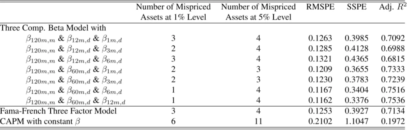
(12) French at http://mba.tuck.dartmouth.edu/pages/faculty/ken.french/. This data set is now rather standard in asset pricing tests and Table 1 displays summary statistics of the monthly returns, in excess of the Treasury bill rate, of these portfolios for our sample period between January 1970 and December 2010. In section 5, we also use 10 portfolios formed on momentum and 30 industry portfolios as additional test assets, which are also available from the same website.. 3. Asset Pricing Performance. We now analyze the performance of the models in explaining the cross-sectional variation in monthly returns on the 25 size and book-to-market sorted portfolios for the period January 1970 to December 2010. We firstly focus on the three component beta models, relative to our two benchmark models; the three factor model of Fama and French (1993, 1996) with constant factor loadings and the unconditional version of CAPM with constant betas. Performance measures discussed in the prior section are displayed in Table 2. The three component beta model with β12m,d , β60m,d and β120m,m has the lowest RMSPE and SSPE and highest adjusted R2 . All three of these performance measures are favorable for this component model, relative to the FamaFrench three factor model and CAPM with constant beta. The adjusted R2 for the component model is 0.7536, compared with 0.7134 for the Fama-French model and 0.1972 for CAPM. Other three component specifications that perform better than the Fama-French model all have the medium-run component set at β60m,d , providing strong support for this factor in explaining the cross-sectional variation in monthly returns. The performance of the three component beta model with β12m,d , β60m,d and β120m,m is very similar to that of the three component beta model with β6m,d , β60m,d and β120m,m , suggesting that either β6m,d or β12m,d is suitable in capturing the short-run component of beta. Table 2 also presents the number of mispriced assets at the 1% and 5% significance levels, based on FamaMacBeth standard errors with Newey-West correction. Again the three component beta model with β12m,d , β60m,d and β120m,m or β6m,d , β60m,d and β120m,m is the best performing model with only one asset mispriced at the 1% significance level. While the Fama-French three factor model has three assets mispriced and the CAPM has six assets mispriced. Table 3 reports the average pricing errors along with their standard errors for each asset. As discussed in Section 2, four sets of standard errors are presented for the benchmark models while only two sets of standard errors are available for the three component beta models. The Fama-MacBeth standard errors with or without Newey-West correction are quite similar to standard errors based on the Shanken correction or the GMM estimation. This suggests that correcting for the errors in variable problem does not significantly affect the standard errors of average pricing errors, at least for the benchmark models.3 In other words, we can conclude that the Fama-MacBeth standard errors, which do not correct for the errors in variables problem, are reliable enough to base our statistical testing of the significance of the average pricing errors from our three component beta models. The Fama-French three factor model fails to explain the return on three portfolios at the 1% significance level: the small-growth portfolio, the fourth size quintile in growth portfolios and the fourth book-to-market quintile in large portfolios. In contrast, the only mispriced asset at the 1% significance level with our three component beta model is the small-growth portfolio, which is known to be the most difficult portfolio to correctly price. Even for this extreme portfolio, the average pricing error based on 3 This is in line with the discussion of the Shanken correction in Section 12.2.3 of Cochrane (2001). He argues that the multiplicative correction term is quite small at the monthly frequency and ignoring it makes little difference.. 10.

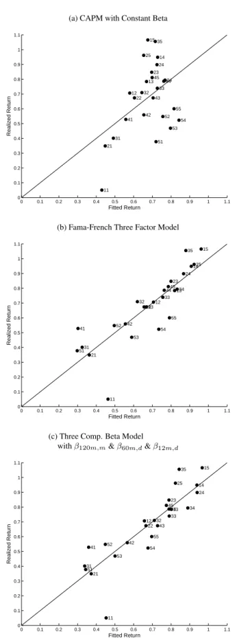
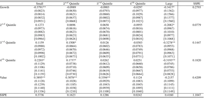
(13) our three component beta model is smaller in absolute value than that based on the Fama-French three factor model. Furthermore, the returns on all other 25 size and book-to-market portfolios are accounted for at the 1% significance level by our three component beta model. Table 3 also reports the SSPE for each size and book-to-market quintile. As is well known, the large pricing errors for the CAPM with constant beta are found to be concentrated in the small, large, growth and value quintiles. Compared to the CAPM with constant betas, the three factor Fama French models does better in accounting for the cross-sectional variation in these quintiles except the growth quintile where the SSPE is 0.2335 compared to 0.2793 for CAPM with constant betas. In contrast, our three component beta model performs better, in terms of SSPE, than the Fama-French three factor model in accounting for the cross-sectional variation in all the extreme quintile portfolios, expect the value portfolios where its performance is only slightly worse than that of the Fama-French three factor model. Pricing performance can also be examined by comparing the average monthly fitted excess return against the average monthly realized excess return for each asset and model. This is displayed in Figure 1 as a plot of fitted versus realized return. Again the deficiencies in the CAPM with constant beta are evident with asset returns deviating sometimes substantially from the 45 degree line. In contrast, the three factor Fama French and three component beta models have asset returns relatively close to the 45 degree line, except for one asset, the small-growth portfolio.. 4. Understanding the Asset Pricing Performance. 4.1. Decomposition of Performance. In this section, we provide some intuition on why the three component beta model performs well. To this end, we analyze the performances of one and two component beta models which allow us to decompose the overall performance of three component beta models. The one component beta models are simply CAPM with betas estimated with different windows and/or frequencies of data. The two component beta models assume that the beta of an asset is a weighted average of two betas estimated with different windows and/or frequencies of data. Panel (a) of Table 4 presents different performance measures of one component beta models. First of all, one component beta models with β1m,d , . . . , β60m,d perform much better than CAPM with constant betas regardless of the performance measure considered. For example, the sum of squared pricing errors for the one component beta model with β60m,d is half that of CAPM while its adjusted R2 is almost threefold that of CAPM. These results suggest that one can explain more than half of the cross-sectional variation in returns by estimating time varying betas based on high frequency data. Secondly, although the one component beta model with β120m,m , the most commonly used approach of capturing time variation in betas, also performs better than CAPM with constant beta, its performance is far less impressive. However, this does not necessarily imply that betas based on low frequency data are completely useless. As we discuss below, they capture a different dimension of the time variation in betas that cannot be captured by betas based on high frequency data. Finally, one can easily analyze the contribution of each beta to the overall performance of the three component beta model by comparing the performance measures of one component beta models to those of three component beta models. Consider the three component beta model with β12m,d , β60m,d and β120m,m as an example. Among the three one component beta models, the one with β60m,d performs better than the one with β12m,d which is in turn better than the one with β120m,m . This suggests that the overall performance of this three component beta model is mostly due to β60m,d and β12m,d , with β120m,m contributing only slightly.. 11.

(14) As discussed in the next section, betas estimated with different windows and/or frequencies of data are, not surprisingly, correlated, although at relatively moderate levels. Hence, the performance measures of one component beta models do not reveal the pure contribution of a specific beta to the overall performance of the three component beta model. Two component beta models allow us to understand the pure contribution of each beta to the overall performance of three component beta models. First, note that two component models perform better than one component models regardless of how betas are estimated. This comparison illustrates the advantages of combining different betas in accounting for the cross-sectional variation in returns. Secondly, two component models where both beta components are estimated using daily data perform better than those where one of the beta components is estimated using monthly data. The best performing two component model, the one with β12m,d and β60m,d , performs almost as well as the Fama-French three factor model. This again demonstrates the advantages of using high frequency data in estimating betas. More importantly, one can easily analyze the pure contribution of each beta to the overall performance of the three component beta model by comparing the performance measures of two component beta models to those of three component beta models. For example, the performance measures of the two component beta model with β60m,d and β120m,m reveal the pure contribution of β12m,d to the overall performance of the three component beta model with β12m,d , β60m,d and β120m,m : (1) The number of assets mispriced at 5% significance levels decreases by one from five to four; (2) The RMSPE and SSPE decrease from 0.1466 and 0.5372 to 0.1162 and 0.3376, respectively; (3) The adjusted R2 increases by almost 15% from 60.88% to 75.36%. To better understand the contribution of each component to the overall performance of three component beta models, we take a closer look at the best performing three component beta model, i.e. the one with β12m,d , β60m,d and β120m,m . To this end, Table 5 presents the percentage decrease in the SSPE due to the inclusion of a specific component. The percentage decrease in the SSPE can be interpreted as a partial R2 since it is the change in the variation explained by the part of that component orthogonal to the other two components. β12m,d and β60m,d decrease the overall SSPE by 37% and 48%, respectively. This is mostly due to their explanatory power for portfolios with high market capitalizations (2nd quintile and above) and book-to-market ratios (3rd quintile and above). They do not significantly decrease the SSPE of portfolios with low book-to-market ratios. The inclusion of β12m,d in the three component beta model actually increases the SSPE of the 2nd quintile of book-to-market sorted portfolios. On the other hand, β120m,m decreases the overall SSPE only by 18%. It performs relatively poorly in explaining the returns on portfolios of small and large and has a mixed performance in explaining the returns on book-to-market sorted portfolios.. 4.2. Dynamics of the Components of Beta. To further our understanding of the asset pricing performance of our three component beta model, we now also study the time variation of beta measurements, β12m,d , β60m,d and β120m,m . Table 7 reports the mean and standard deviation of these beta components for the 25 size and book-to-market sorted portfolios over our sample period between January 1970 to December 2010. In regard to the means of these betas, there is a strong pattern in all three beta measurements, in the form of a decreasing mean beta as the book-to-market ratio of a portfolio increases. This suggests that the mean betas cannot possibly account for the fact that portfolios with higher book-to-market ratios also have higher mean returns as presented in Table 1. Although not presented, this is also in line with the pattern observed in constant betas estimated once using the whole sample. On the other. 12.

(15) hand, there is no clear pattern in the mean of all three beta components as functions of the market capitalization of a portfolio. Similar to their constant betas, the mean of the long term beta component, β120m,m , increases as the market capitalization of a portfolio decreases. This suggests that the mean of the long term beta component might account for the fact that portfolios with smaller market capitalizations have higher mean returns as presented in Table 1. However, the same cannot be said about the mean of short- and medium-term beta components. There is no clear pattern in the mean of short- and medium-term beta components. More importantly, if there is any pattern, it tends to work in the opposite direction with large firms having higher betas than small firms. To summarize, these results suggest that variation in the means of different beta components cannot possibly account for the observed patterns in mean returns. Instead, results on the variability of beta will contribute to providing an explanation to the success of our three component beta model. To see this, Table 7 presents the standard deviation of different beta components. The standard deviation of β12m,d , β60m,d and β120m,m increases as the market capitalization of a portfolio decreases and its book-to-market ratio increases. For example, for the short-run beta component, the standard deviation of the large-growth portfolio is 0.1407, compared with 0.2590 for the small-value portfolio. For the long-run beta component, the standard deviation for the large-growth and small-value portfolios are 0.0408 and 0.1872, respectively. In addition, summary statistics on the annual changes in β12m,d for the 25 size and book-to-market sorted portfolios over the January 1970 to December 2010 are presented in Table 9. The variability of these beta changes in respect to standard deviation, minimum, maximum and range provide insights into the relationship between the dynamics of beta and returns. In particular, as the book-to-market ratio of a portfolio increases, the maximum annual beta change tends to rise. For example, the maximum annual change for the small-growth portfolio is 0.5590, whereas the maximum annual change for the smallvalue portfolio is 0.7736. For the large-growth and large-value portfolios, the maximum annual change is 0.2169 and 0.8132, respectively. A pattern in the variability of beta changes also exists in relation to the market capitalization of a portfolio. As the market capitalization of a portfolio increases, the range of annual beta changes (maximum minimum) increases. For example, the range of the small-growth portfolio is 1.2147, whereas the range of the largegrowth portfolio is 0.5264. The recent financial crisis also provides further insights and Table 8 reports the mean and standard deviation of β12m,d , β60m,d and β120m,m for the 25 size and book-to-market sorted portfolios over the period, January 2009 to December 2010. During this period there is a dramatic change in the pattern of mean betas for β12m,d and β60m,d . In particular for β12m,d there is now a strong pattern of an increasing mean beta as the market capitalization of the portfolio decreases and its book-to-market ratio increases. For example, the mean of β12m,d is 0.7914 for the large-growth portfolio and 1.1699 for the small-value portfolio. This reversal in the pattern of beta, relative to that over the full sample, demonstrates the dramatic changes in beta during the turmoil of the financial crisis. These summary statistics suggest that the variability in beta is related to the size and value premia that are evident in the mean returns of the 25 size and book-to-market sorted portfolios. Part of the success of our three component beta component model can be attributed to capturing these beta dynamics. We next investigate the annual change in each beta component, β12m,d , β60m,d and β120m,m , in relation to the business cycle. Table 10 displays the correlations of the annual beta changes with the Treasury bill rate, for our 25 size and book-to-market sorted portfolios over the January 1970 to December 2010. The Treasury bill rate at the beginning of the 12 month period is chosen for measuring economic conditions over the next 12 months. Panel a displays the correlations for the annual changes of β12m,d which are mostly insignificant, indicating that the dynamics of the short-. 13.

(16) run component are not dominated by the business cycle. In contrast, panel b and c display a number of significant correlations for annual changes of β60m,d and β120m,m with the Treasury bill rate. A strong pattern is present where correlations become significantly more negative as the book-to-market ratio of the portfolio increases, with the most significant negative correlations being approximately -0.5. Thus, in recessions when the Treasury bill rate is low, the medium- and long-run beta components for portfolios with high book-to-market ratios, tend to rise over the year. It is widely acknowledged that the business cycle has significant impacts on asset returns, and in our three component beta model this is primarily captured through the medium- and long-run beta components. It is not too surprising that the business cycle is not primarily driving the short-run beta component, as typically the dynamics of the business cycle are slowly changing, whereas the short-run beta component is designed to capture fast moving beta dynamics. For example, changes in a portfolio’s specific risk characteristics are likely to be more immediate in nature and have a more rapid impact on the portfolio’s short-run beta component. To illustrate this, Table 11 displays the correlations of 11 month changes in betas with the prior 12 month change in the value-weighted average book-to-market ratio of the portfolio. The 11 month change in an asset’s beta component is measured from 1 July to 1 June so that the asset composition remains unchanged, as rebalancing of portfolios occurs at the beginning of July. The prior 12 month change in the value-weighted average book-to-market ratio of the portfolio is from 1 July and is obtained from the Kenneth French Data Library. This 12 month change in the book-to-market ratio of the portfolio captures the change in one of the important portfolio characteristics. Panel a of Table 11, displays correlations for the short-run beta component of the 25 size and book-to-market sorted portfolios, showing highly significant positive correlations for the value portfolios with the highest correlation being 0.6329. Overall, there is a pattern of increasing correlation as the book-to-market ratio of the portfolio increases. Demonstrating that an increase in the portfolio’s risk characteristics due to an increase in its book-to-market ratio, often results in significant increases in the short-run beta component. Panels b and c of Table 11 display correlations for the medium- and long-run beta components with mostly insignificant correlations, showing that these beta components are less sensitive to the more fast moving risk dynamics of assets. Finally, Table 6 presents summary statistics on the correlations between the short-, medium- and long-run beta components for the 25 size and book-to-market sorted portfolios. These correlations are typically not too high, with the highest mean correlation being 0.6823 which is between the short- and medium-run beta components, and the lowest mean correlation being 0.1220 which is between the short- and long-run beta components. These relatively moderate levels of correlation between different components of beta suggest that they do indeed capture different frequency variations in betas.. 5 5.1. Robustness Checks Some Simulation Results. Lewellen, Nagel, and Shanken (2010) argue that it is relatively easy to come up with factors that explain most of the cross-sectional variation in the 25 size and book-to-market portfolios due to the strong factor structure in these portfolios. Specifically, they generate different types of artificial factors and show that these artificial factors can explain the cross-sectional variation in the 25 size and book-to-market portfolios as well as the Fama-French three factor model. They provide several suggestions to remedy this problem. We implement some of these suggestions to. 14.

(17) to show that the performance of our three component beta model relative to the Fama-French three factor model is not due to this strong factor structure in the 25 size and book-to-market portfolios. Before considering their suggestions, we start in this section with a simulation exercise similar to theirs and analyze whether the relative success of our three component beta model is due to the possibility that it might be exploiting the strong factor structure present in the 25 size and book-to-market portfolio. In our framework, instead of several factors with constant loadings, there is only one factor, the return on the market portfolio, whose loading is assumed to be time-varying and measured as a weighted average of loadings estimated over different window of observations with different frequencies. Hence, we generate only two artificial factors replacing the daily and monthly observations of the return on the market portfolio. Specifically, let ωt denote a 3 × 1 vector of random weights drawn from a standard normal distribution. We generate artificial factors as Pt = ωt′ Ft + vt where Ft is a 3 × 1 vector of either daily or monthly Fama-French factors and vt is another random variable independent of ωt′ and Ft . We then estimate the three component beta model with β12m,d,t , β60m,d,t and β120m,m,t based on the time series of daily and monthly artificial factors. We repeat this exercise 5,000 times and report the summary statistics for different performance measures in Table 12. First of all, there are, on average, five to six (two to three) mispriced assets at the 5% (1%) level when we use artificial factors to account for the cross-sectional variation in the 25 size and book-to-market portfolios. Secondly, the RMSPE and SSPE based on artificial factors are, on average, 0.1555 and 0.6118, respectively. Thirdly, the average adjusted R2 based on artificial factors is 0.5536, suggesting that artificial factors can explain a little more than half of the cross-sectional variation in the 25 size and book-to-market portfolios. These results are consistent with those in Lewellen, Nagel, and Shanken (2010) who also find that artificial factors can explain a non-negligible part of the cross-sectional variation in the 25 size and book-to-market portfolios. However, the explanatory power of artificial factors are still, on average, well below that of our three component beta models. For example, the three component beta model with β12m,d,t , β60m,d,t and β120m,m,t has an RMSPE of 0.1162, a SSPE of 0.3376 and an adjusted R2 of 0.7536. More importantly, the performance measures of our three component beta models are outside the 5% and 95% quantiles of these performance measures based on artificial factors. In other words, the probability that the relative success of our three component beta models is due to luck is less than 5%.. 5.2. Additional Test Portfolios. We now turn our attention to analyzing the performance of the models in explaining the cross-sectional variation in monthly returns with additional test portfolios, namely the 10 momentum sorted portfolios and 30 industry portfolios, from the Kenneth French Data Library. Performance of the three component beta models as well as the two benchmark models, CAPM with constant beta and the Fama-French three factor model, is again evaluated for the period January 1970 to December 2010. Performance measures for the pricing of the 25 size and book-to-market cross sorted portfolios, 10 momentum sorted portfolios and 30 industry portfolios are displayed in Table 13. These results firstly show that when all these assets are priced, there is a substantial increase in pricing errors across all models, relative to the pricing of just the 25 size and book-to-market cross sorted portfolios. For example, the adjusted R2 for the best performing three component beta model, Fama-French three factor model and CAPM is 0.3692, 0.2699 and 0.0792, respectively. Whereas, for the pricing of just the 25 size and book-to-market cross sorted portfolios, the adjusted R2 for the models are 0.7536, 0.7134 and 0.1972, respectively. This substantial increase. 15.

(18) in pricing errors is largely attributed to the inclusion of the industry portfolios, which exhibit relatively little cross sectional dispersion in average returns as shown in Santos and Veronesi (2006). As discussed in Lewellen, Nagel, and Shanken (2010), assessing the performance of asset pricing models on additional portfolios to the size and book-tomarket cross sorted portfolios, raises the hurdle in evaluating model performance. In this regard, our three component beta models start to demonstrate outperformance, relative to the Fama-French three factor model. The best performing three component beta model is with β3m,d , β12m,d and β120m,m based on RMSPE, SSPE and adjusted R2 . The number of assets that this model misprices at the 1% significance level is 6. While the Fama-French three factor model misprices 8. The performance of the three component beta model with β12m,d , β60m,d and β120m,m is again very similar to that of the three component beta model with β6m,d , β60m,d and β120m,m and the number of assets that these models misprice at the 1% significance level is also 6. The RMSPE, SSPE and adjusted R2 of these two models is comparable with the Fama-French three factor model, however, they do not outperform the three component beta model with β3m,d , β12m,d and β120m,m . Thus, the inclusion of these additional portfolios, favors beta component models with short- and medium-run components measured over a shorter period. This is consistent with substantial time variation in industry betas, which has been found in earlier studies such as Ferson and Harvey (1991) and Braun, Nelson, and Sunier (1995).. 5.3. Alternative Frequencies. In this section, we analyze whether the three component beta models continue to perform just as well as the FamaFrench three factor model in accounting for the cross-sectional variation in quarterly returns on the 25 size and bookto-market cross sorted portfolios. To this end, we use monthly returns on these portfolios to calculate their quarterly returns. We then estimate the three component beta models as well as the benchmark models using quarterly instead of monthly returns. Table 14 presents the performance measures for the three component beta models and the benchmark models. Before comparing the performances of the three component beta models to those of the Fama-French three factor model, we should first note that the RMSPE and SSPE are higher than those based on monthly returns, regardless of the model considered, since quarterly returns are higher on average than monthly returns. Furthermore, compared to the results based on monthly returns, there is a deterioration in the performance of CAPM with constant betas when we consider quarterly returns, while the other models continue to perform similarly. For example, the adjusted R2 of the CAPM with constant betas based on quarterly returns is only 6% compared to an adjusted R2 of 19% based on monthly returns. More importantly, the results in Table 14 suggest that the three component beta models continue to perform as well as or even sometimes better than the Fama-French three factor model in accounting for the cross-sectional variation in quarterly returns on the 25 size and book-to-market cross sorted portfolios. First of all, the best performing three component beta model for monthly returns, namely the one with β12m,d , β60m,d and β120m,m , performs as well as the Fama-French three factor model based on RMSPE, SSPE and adjusted R2 and outperforms it based on the number of significantly mispriced assets. Secondly, two similar three component beta models where we replace β12m,d with either β6m,d or β3m,d actually outperform the Fama-French three factor model based on all measures. These results suggest that three component beta models are as good of a model or even a better one than the Fama-French three. 16.

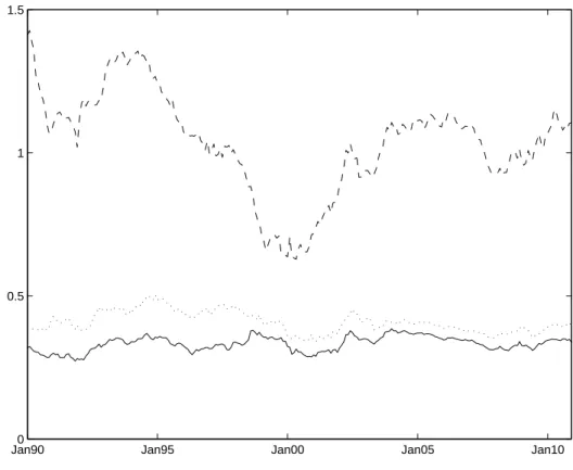
(19) factor model in accounting for the cross-sectional variation in both monthly and quarterly returns.. 5.4. Alternative Sample Periods. In this section, we analyze how the best performing three component beta model fairs against the benchmark models especially the Fama-French three factor model over different sample periods. To this end, we firstly analyze the performances of these models over an expanding window of sample periods starting with the first sample period between January 1970 and January 1990. Given that an increasing number of observations generally improves precision in estimating sample means, we consider an expanding rather than rolling window of observations in estimating average pricing errors, which are simply the sample averages of conditional alphas. Figure 2 presents the SSPE of the three component beta model with β12m,d , β60m,d and β120m,m and the two benchmark models for the period between January 1990 and December 2010. The SSPEs of the three component beta model and the Fama-French three factor model are quite stable over different sample periods, whereas that of the CAPM model is less stable. Specifically, CAPM performs performs better when we consider sample periods between 1970 and the second half of the 90s, but its performance decreases, i.e. its SSPE increases, as we add data from the 2000s. More importantly, the three component beta model with β12m,d , β60m,d and β120m,m performs always better than the Fama-French three factor model, which in turn performs better than the CAPM with constant betas, as we consider an expanding window of observations. To summarize, the three component beta model does not only have a stable performance in accounting for the cross-sectional variation in returns but also its success relative to the Fama-French three factor model is not due to the specific sample period considered in Section 3 and 4. Secondly, we analyze the performances of these models over expansion and recession periods during the business cycle. We classify a month as either part of the expansion or recession phase through the NBER classification. Table 15 presents the SSPE of the three component beta model with β12m,d , β60m,d and β120m,m and the two benchmark models for each portfolio quintile, over both the expansion periods (displayed in panel a), and over the recession periods (displayed in panel b.) During expansions, the SSPE of the three component beta model is very similar to that of the Fama-French three factor model, over all quintiles. However, during recessions (when pricing errors rise for all the models) the SSPE of the three component beta model is lower relative to that of the Fama-French three factor model. The largest differences in SSPE between these two models in recessions occurrs in the growth and value quintiles. For the growth quintile, the SSPE’s for the two models are 0.3197 and 0.5173, respectively. And for the value quintile, the SSPE’s for the two models are 0.2048 and 0.4000, respectively. The three component beta model in recessions also produces substantially lower SSPE’s for the small and large quintiles. This suggests that the three component beta model does a relatively good job in capturing dynamics during recessions. In contrast, the two benchmark models have inferior performance. The SSPE for CAPM with constant betas in expansions and recessions is 1.0112 and 2.1113, respectively. The SSPE for the Fama-French three factor model in expansions and recessions is 0.3496 and 1.1480, respectively. Whereas, the SSPE for the three component beta model in expansions and recessions is 0.3561 and 0.8037, respectively.. 5.5. Nonsynchronous Trading. Lo and MacKinlay (1990) point out that nonsynchronous price movements in stocks can occur due to small stocks having delayed price reactions. While these effects can be important for individual stocks, the impact for broadly. 17.

(20) diversified value-weighted portfolios is much less. However, to ensure our results are not biased, due to nonsynchronous trading, we conduct two further robustness tests. Firstly, we simply remove the 5 test portfolios from the small quintile from the 25 size and book-to-market cross sorted portfolios. Performance measures of the models for the pricing of the remaining 20 size and book-to-market cross sorted portfolios for the period January 1970 to December 2010 are displayed in Table 16. Overall, the pricing performance of the Fama-French three factor model and the the three component beta model with β12m,d,t , β60m,d,t and β120m,m,t remain comparable over the different performance measures. Both models have lower pricing error from the remove of these 5 test portfolios. The Fama-French three factor model adjusted R2 rises from 0.7134 to 0.8050. While the three component beta model adjusted R2 rises from 0.7536 to 0.8195. Thus, we can conclude that the 5 small test portfolios are not highly influential in the performance measurements of the three component beta model. In addition, to further examine potential bias from nonsynchronous trading, we follow the approach of Dimson (1979) and Lewellen and Nagel (2006) and estimate our short- and medium-run beta components from daily returns using the following regression equation. Ri,t = αi + βi0 Rm,t + βi1 Rm,t−1 + βi2 [(Rm,t−2 + Rm,t−3 + Rm,t−4 )/3] + +ui,t. (21). with βi = βi0 + βi1 + βi2 . We then re-run our analysis of the component beta models over the 25 size and book-tomarket cross sorted portfolios, with performance measures displayed in Table 17, showing relatively little change due to this correction for nonsynchronous trading. For example, the adjusted R2 for the the three component beta model with β12m,d,t , β60m,d,t and β120m,m,t only falls from 0.7536 to 0.7325.. 6. Conclusions. The prior literature on empirically assessing asset pricing models has most commonly measured systematic risk with monthly returns and as a single component. In this paper, we propose to model the conditional beta of an asset as a weighted average of three betas estimated over different periods using different frequency data. Our three component beta model can be considered as a mixed-frequency approach as the short- and medium-run beta components are computed from daily returns, whereas, the long-run beta component is computed from monthly returns. We demonstrate that much can be gained when daily and monthly returns are utilized to measure components of systematic risk in an asset pricing framework. Specifically, we show that our three component beta model can account for the crosssectional variation in expected returns, just as well as the Fama-French three factor model. Most of the gain occurs through the use of daily returns and thus an important implication of this study is that when accurate daily returns are available, they should be utilized in CAPM applications. Our results also suggest that the more immediate changes in risk such as changes in portfolio characteristics are captured in the short-run beta component while the medium- and long-run beta components capture more slowly changing risk which we find to be correlated with the business cycle. The empirical success of our three component beta model relative to the Fama-French three factor is partly due to its success in capturing time-variation in risk of portfolios in recessions.. 18.

(21) References Adrian, Tobias, and Joshua Rosenberg, 2008, Stock returns and volatility: pricing the short-run and long-run components of market risk, Journal of Finance 63, 2997–3030. Andersen, Torben G., Tim Bollerslev, Francis X. Diebold, and Ginger Wu, 2005, A framework for exploring the macroeconomic determinants of systematic risk, American Economic Review 95, 398–404. , 2006, Realized beta: persistence and predictability, Advances in Econometrics: Econometric Analysis of Economic and Financial Times Series in Honour of R.F. Engle and C.W.J. Granger B, 1–40. Ang, Andrew, and Joseph Chen, 2007, Capm over the long run: 1926-2001, Journal of Empirical Finance 14, 1–40. Berk, Jonathan B., Richard C. Green, and Vasant Naik, 1999, Optimal investment, growth options, and security returns, Journal of Finance 54, 1553–1607. Braun, Phillip A., Daniel B. Nelson, and Alain M. Sunier, 1995, Good news, bad news, volatility, and betas, Journal of Finance 50, 1575–1603. Cochrane, John H., 1996, A cross-sectional test of an investment-based asset pricing model, Journal of Political Economy 104, 572–621. , 2001, Asset Pricing (Princeton University Press: Princeton, NJ). Dimson, Elroy, 1979, Risk measurement when shares are subject to infrequent trading, Journal of Financial Economics 7, 197–226. Engle, Robert F., and Jose Gonzalo Rangel, 2010, High and low frequency correlations in global equity markets, Stern School of Business, New York University, Working Paper. Fama, Eugene F., and Kenneth R. French, 1993, Common risk factors in the returns on bonds and stocks, Journal of Financial Economics 33, 3–56. , 1996, Multifactor explanations of asset pricing anomalies, Journal of Finance 51, 55–84. Fama, Eugene F., and James D. MacBeth, 1973, Risk, return, and equilibrium: empirical tests, Journal of Political Economy 81, 607–636. Ferson, Wayne E., and Campbell R. Harvey, 1991, The variation of economic risk premiums, Journal of Political Economy 99, 385–415. , 1993, The risk and predictability of international equity returns, Review of Financial Studies 6, 527–566. , 1999, Conditioning variables and the cross-section of stock returns, Journal of Finance 54, 1325–1360. Ghysels, Eric, and Eric Jacquier, 2006, Market beta dynamics and portfolio efficiency, HEC Montreal, Working Paper. Hamada, Robert S., 1972, The effects of the firm’s capital structure on the systematic risk of common stocks, Journal of Finance 27, 435–452.. 19.

(22) Harvey, Campbell R., 1989, Time-varying conditional covariances in tests of asset pricing models, Journal of Financial Economics 24, 289–317. , 2001, The specification of conditional expectations, Journal of Empirical Finance 8, 573637. Hooper, Vincent J, Kevin Ng, and Jonathan J Reeves, 2008, Quarterly beta forecasting: an evaluation, International Journal of Forecasting 24, 480–489. Jagannathan, Ravi, and Zhenyu Wang, 1996, The conditional capm and the cross-section of expected returns, Journal of Finance 51, 3–53. Lettau, Martin, and Sydney Ludvigson, 2001, Resurrecting the (c)capm: a cross-sectional test when risk premia are time-varying, Journal of Political Economy 109, 1238–1287. Lewellen, Jonathan, and Stefan Nagel, 2006, The conditional capm does not explain asset-pricing anomalies, Journal of Financial Economics 82, 289–314. , and Jay Shanken, 2010, A skeptical appraisal of asset pricing tests, Journal of Financial Economics 96, 175–194. Lo, Andrew W., and A. Craig MacKinlay, 1990, When are contrarian profits due to stock market overreaction, Review of Financial Studies 3, 175–205. Newey, Whitney K., and Kenneth D. West, 1987, A simple, positive semi-definite, heteroskedasticity and autocorrelation consistent covariance matrix, Econometrica 55, 703–708. Rangel, Jose Gonzalo, and Robert F. Engle, 2009, The factor-spline-garch model for high- and low-frequency correlations, Stern School of Business, New York University, Working Paper. Rubinstein, Mark E., 1973, A mean-variance synthesis of corporate financial theory, Journal of Finance 28, 167–181. Santos, Tano, and Pietro Veronesi, 2006, Labor income and predictable stock returns, Review of Financial Studies 19, 1–44. Shanken, Jay, 1990, Intertemporal asset pricing: an empirical investigation, Journal of Econometrics 45, 99–120. , 1992, On the estimation of beta-pricing models, Review of Financial Studies 5, 1–55.. 20.

(23) Figure 1: Realized vs Fitted Returns (a) CAPM with Constant Beta 1.1 15 35 1 25. 14. 0.9. 24. 0.8. 13. 23 45. 34 44. Realized Return. 33 32 12 22. 0.7. 43 55. 0.6 42. 52. 41. 0.5. 54 53. 31. 0.4. 51. 21 0.3 0.2 0.1 11 0. 0. 0.1. 0.2. 0.3. 0.4. 0.5. 0.6. 0.7. 0.8. 0.9. 1. 1.1. Fitted Return. (b) Fama-French Three Factor Model 1.1 15. 35 1 1425 0.9. 24 23 45 34 44 13. 0.8. Realized Return. 33 32. 0.7. 12 22 43 55. 0.6 52. 41. 0.5. 42 54 53. 31 51. 0.4. 21. 0.3 0.2 0.1 11 0. 0. 0.1. 0.2. 0.3. 0.4. 0.5. 0.6. 0.7. 0.8. 0.9. 1. 1.1. Fitted Return. (c) Three Comp. Beta Model with β120m,m & β60m,d & β12m,d 1.1 15. 35 1 25. 14. 0.9. 24 23 45 44 13 33. Realized Return. 0.8. 34. 12 32 22 43. 0.7. 55. 0.6 41. 0.5. 42. 52. 54 53. 31 51. 0.4. 21. 0.3 0.2 0.1 11 0. 0. 0.1. 0.2. 0.3. 0.4. 0.5. 0.6. 0.7. 0.8. 0.9. 1. 1.1. Fitted Return. Note: This figure plots average monthly realized excess returns on the 25 size and book-to-market returns in the y-axis against their fitted values from three asset pricing models in the x-axis. The numbers on the graphs refer to individual portfolios with the first number denoting the size and the second number denoting the book-to-market quintile.. 21.

(24) Figure 2: SSPE of Asset Pricing Models for Alternative Sample Periods. 1.5. 1. 0.5. 0 Jan90. Jan95. Jan00. Jan05. Jan10. Note: This figure presents the SSPE for 25 size and book-to-market portfolios from asset pricing models over an expanding window of observations starting with the first window between January 1970 and January 1990 and ending with the last window between January 1970 and December 2010. The dashed, dotted and solid lines correspond to the SSPEs of the CAPM with constant betas, the Fama-French three-factor model and the three component beta model with β12m,d , β60m,d and β120m,m , respectively.. 22.