THESE PAR ARTICLES PRÉSENTÉE À L'ÉCOLE DE TECHNOLOGIE SUPÉRIEURE
COMME EXIGENCE PARTIELLE À L'OBTENTION DU DOCTORAT EN GÉNIE
Ph.D.
PAR
KECHROUD, Riyad
UNE METHODE DE COUPLAGE ELEMENTS FINIS- CONDITIONS ABSORBANTES DE TYPE-PADÉ POUR LES PROBLÈMES DE DIFFRACTION
ACOUSTIQUE
MONTREAL, LE 16 JANVIER 2008
Professeur, Azzeddine Soulaïmani, directeur de thèse
Département de génie mécanique à École de technologie supérieure
Professeur, Ammar B. Kouki, président du jury
Département de génie électrique à École de technologie supérieure
Professeur, Marins Paraschivoiu, examinateur exteme Département de génie mécanique à l'Université Concordia
Professeur, Frédéric Laville, examinateur
Département de génie mécanique à École de technologie supérieure
ELLE A FAIT L'OBJET D'UNE SOUTENANCE DEVANT JURY ET PUBLIC LE 7 JANVIER 2008
KECHROUD, Riyad SOMMAIRE
Nous nous intéressons aux problèmes harmoniques de diffraction acoustique en milieu infini régis par l'équation de Helmholtz. La simulation numérique de ces phénomènes est complexe notamment lorsqu'il est question de fréquences élevées et d'obstacles de forme allongée tel qu'un sous-marin. Les codes éléments finis commerciaux sont incapables de cerner tous les aspects liés à ce type de problèmes. De plus, ce genre d'applications fait ap-pel à de grandes ressources de calcul. En effet, la taille du système d'équations à résoudre (plusieurs millions de ddl) engendre souvent l'épuisement des ressources des calculateurs traditionnels.
Notre objectif est de solutionner ce type de problèmes avec une précision pratique en utili-sant le minimum de ressources. Nous proposons ainsi une méthode de couplage éléments finis de type Lagrange et à base d'ondes planes avec les conditions absorbantes d'ordre élevé basées sur les approximants complexes de Padé. A travers une série d'expériences numériques, nous montrons l'efficacité de ces conditions absorbantes en comparaison avec les conditions absorbantes de Bayliss-Gunzburger-Turkel d'ordre deux implémentées dans les codes commerciaux. La méthodologie proposée permet non seulement une réduction de la taille du domaine de calcul sans dégradation de la précision mais conduit également à la résolution de systèmes d'équations de taille relativement réduite.
KECHROUD, Riyad ABSTRACT
We address problems of acoustic diffraction in infinité médium govemed in the harmonie régime by the Helmholtz équation. The simulation of thèse phenomena is complex espe-cially when it involves higher frequency and elongated scatterers such as a submarine. The finite élément commercial codes are unable to deal with ail the aspects related to this kind of problems. Moreover, this kind of applications requires a huge amount of computational resources. Indeed, the size of the System of équations to be solved (several million ddl) often overwhelm the resources of the most available calculators.
Our goal is to solve this kind of problems with an engineering accuracy using the minimum of resources. We thus propose a method coupling plane wave and Lagrange finite éléments with higher order Padé-type absorbing boundary conditions. Through a séries of numerical experiments, we show the effectiveness of thèse absorbing conditions in comparison with the second order Bayliss-Gunzburger-Turkel absorbing boundary conditions implemented in the commercial codes. This methodology allows us not only to reduce the size of the computational domain without degrading the précision but also lead us to the solution of Systems of reduced size.
Je remercie toutes les personnes de prés ou de loin qui m'ont aidé à l'aboutissement de cette thèse.
Je voudrais exprimer ma gratitude au Professeur Azzeddine Soulaïmani pour m'avoir pro-posé ce thème de recherche et d'en avoir assumé la direction. Ses conseils éclairés m'ont permis de progresser mais surtout d'apprendre, merci pour la patience et pour le support inconditionnel.
Je voudrais également remercier le Professeur Ammar B. Kouki, pour avoir accepté d'être président de ce jury de thèse, et les Professeurs Marins Paraschivoiu et Frédéric Laville pour avoir accepté d'évaluer ce travail.
Je tiens aussi à remercier les Professeurs Youssef Saad et Xavier Antoine pour la collabo-ration fructueuse que nous avons eu.
Je tiens également à remercier tous les membres du groupe GRANIT, où j'ai trouvé un environnement humain idéal pour la recherche. Que mes amis et collègues Aminé Benhaj Ali, Riadh Ata, Youcef Bouchera, Youcef Loukili, Nizar El-Houssaïni, Jack Feng, Simon Nicolas Roth, Adile et Jean-Marie trouvent ici l'expression de ma gratitude.
Je ne saurais oublier l'appui inconditionnel de toute ma famille. Je voudrais remercier en particulier ma conjointe Nassima et ma petite fille Aya. Je vous dédie ce travail.
Je voudrais reconnaître l'appui financier de mon directeur de thèse et celui de l'École de Technologie Supérieure.
Page
SOMMAIRE.
ABSTRACT h REMERCIEMENTS iii
TABLE DES MATIÈRES v LISTE DES TABLEAUX viii LISTE DES FIGURES xii LISTE DES ABRÉVIATIONS ET SIGLES xv
INTRODUCTION GÉNÉRALE 1 CHAPITRE 1 PRECONDITIONING TECHNIQUES FOR THE SOLUTION
OF THE HELMHOLTZ EQUATION BY THE FINITE
ELE-MENT METHOD 14 1.1 Mathematical model 17 1.1.1 General model 17 1.1.2 DtN boundary conditions 18
1.1.3 Variational formulation 19 1.1.4 Analytic and Numerical computation of the parameter r 20
1.2 Solution method 21 1.3 Numerical Experiments in 2D 24
1.3.1 Impact of discretization 27 1.3.2 Impact of the dropping strategy in ILU type precondtioners 29
1.3.3 Performance of GMRES-ILUT for différent frequency régimes 32
1.3.4 Performance of différent preconditioners for GMRES 35 1.3.5 Computing preconditioners from problems with lower wavenumbers ... 35
1.4 Numerical Experiments in 3D 36 1.4.1 Problem 1 : Dirichlet Problem 38 1.4.2 Problem 2 : Neumann Problem 39 1.4.3 Impact of the discretization scheme 40
BIBLIOGRAPHIE 45 CHAPITRE 2 NUMERICAL ACCURACY OF A PADÉ-TYPE NON-REFLECTING
BOUNDARY CONDITION FOR THE FINITE ELEMENT SOLUTION OF ACOUSTIC SCATTERING PROBLEMS AT
HIGH-FREQUENCY 48 2.1 Exact and approximate mathematical models 53
2.1.1 The two-dimensional exterior acoustic scattering problem 53 2.1.2 Formulation in a bounded domain with the BGT2-like NRBC 54 2.2 A high-order Padé-type ABC for high-frequency scattering 56
2.3 Itérative Krylov finite élément solution 60
2.3.1 Variational formulation 60 2.3.2 The Galerkin-Least-Squares finite élément method 61
2.3.3 Preconditioned itérative Krylov scheme 62 2.4 Performances and comparisons for some model test problems 64
2.4.1 The sound-hard circular cylinder 65 2.4.2 The sound-hard elliptical cylinder 72 2.5 Sound-hard submarine-shaped scatterer 76 2.6 A few words on the computational aspects 79
2.7 Conclusion 84 BIBLIOGRAPHIE 85 CHAPITRE 3 PERFORMANCE STUDY OF PLANE WAVE FINITE
ELE-MENT METHODS WITH A PADÉ-TYPE ARTIFICIAL
BOUN-DARY CONDITION IN ACOUSTIC SCATTERING 91
3.1 A Padé-type artificial boundary condition 94 3.1.1 The two-dimensional scattering problem 94 3.1.2 Bounding the domain by using a Padé-type ABC 95
3.1.3 Variational formulation with Padé-type ABC 97
3.2 Finite élément approximation 99
3.3 Numerical study 101 3.3.1 The circular cylinder 102 3.3.2 The sound-hard elliptical cylinder 107
3.3.3 The submarine-like shaped scatterer 111
3.4 Conlusion 121 BIBLIOGRAPHIE 122 CONCLUSION GÉNÉRALE 128
ANNEXE A ON THE THREE-DlMENSlONAL SCATTERING PROBLEM 132
A. 1 The three-dimensional scattering problem 132 A. 1.1 Bounding the domain by using a Padé-type ABC 133 A.1.2 Variational formulation with Padé-type ABC 135
A.2 Finite élément approximation 136 A.2.1 Implementation of the Padé non-reflecting boundary condition 137
A.3 Numerical study 140 ANNEXE B POIDS ET POINTS D'INTÉGRATION 142
B.l Points et poids d'intégration de Gaussen ID 142 B.1.1 Abscisses des points d'intégration de Gaussen ID 142 B.l.2 Poids des points d'intégration de Gauss en ID 143 B.2 Points et Poids d'intégration de Gauss en 2D 143 B.3 Points et poids d'intégration de Gauss en 3D 144 ANNEXE C MÉTHODE GMRES ET SES PRÉCONDITIONNEURS 146
C. 1 Méthode GMRES pour systèmes à nombres complexes 146 C.2 Préconditionneurs algébriques ILUO, ILUT et ILUTC 146
C.3 Préconditionneurs déflatés 146
Page
Table 1.1 Numerical results for problem 1 with ILUT-GMRES 26 Table 1.2 Error in the finite élément solution for Galerkin and Galerkin
Least-squares(GLS) discretization schemes for différent mesh-sizes. The values in the parenthesis correspond to GLS scheme.
Order 2 Bayliss-Turkel boundary conditions used 28 Table 1.3 Itération count (Iter) and CPU time (Time) versus the If il
parameter of ILUT. Tolérance is set to l.e-05. GLS scheme
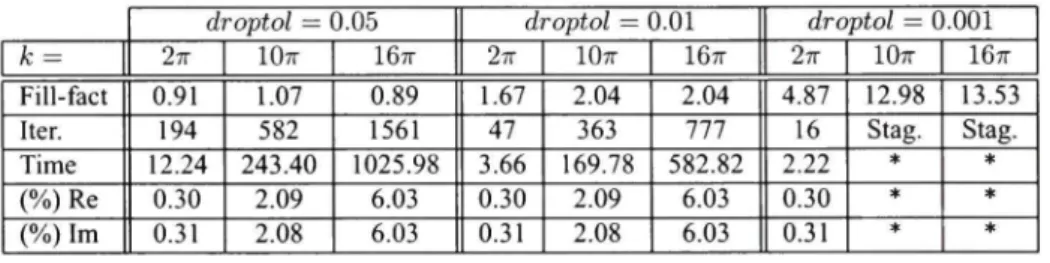
results between parenthèses 30 Table 1.4 Performance of ILUT using If il = 8 x nnz/n, im=50
when droptol is varied, for Systems associated with différent
wavenumbers (Standard Galerkin scheme) 31 Table 1.5 Performance of ILUTP(ILUT with pivoting) using If il =
8 X nnz/n, im=50, and permtol=0.1, when droptol is varied, for Systems associated with différent wavenumbers (Standard
Galerkin scheme) 31 Table 1.6 Behavior of ILUT-preconditioned GMRES for différent
wavenumbers and différent mesh sizes 32 Table 1.7 Behavior of ILUT-preconditioned GMRES for a wave number
Â;=l 67r and two différent mesh resolutions. Case If il = 1 33 Table 1.8 Itération count (Iter) and CPU time (Time) versus the Ifil
parameter of ILUT. GLS scheme results between parenthèses 33 Table 1.9 Itération count (Iter) and CPU time (Time) versus the Ifil for
différent preconditioners 36 Table 1.10 Performances of the solvers ILUT-GMRES and ILUO-GMRES
for différent wavenumbers and différent mesh sizes (Soft Scatterer) 39 Table 1.11 Performances of the solver ILUT-GMRES vs. ILUO-GMRES
Table 1.12 Performances of the solver ILUT-GMRES for différent
différent mesh sizes (Galerkin and GLS Scheme) 42 Table 2.1 RMS relative error on the interior solution (on the trace) of the
computed scattered field for différent values of the parameters defining the Padé-type ABC and the BGT-like ABC. The mesh
resolution is fixed to n\ = 40 and m, = 1/4 for the Galerkin scheme 66 Table 2.2 RMS relative error on the interior solution (on the trace) of the
computed scattered field for différent values of the parameters defining the Padé-type ABC and the BGT-like ABC. The mesh resolution is fixed to nx = 40 and m = 1 for the Galerkin
scheme 67 Table 2.3 Circular cylinder : RMS error for différent mesh resolutions
of the Galerkin FEM and ABC positions. The values in
parenthesis correspond to the error on the trace 67 Table 2.4 Circular cylinder : RMS error for différent mesh resolutions of
the GLS22.5 FEM and ABC positions. The values in parenthèses
correspond to the error on the trace 68 Table 2.5 Circular cylinder : RMS error for différent mesh resolutions
of the GLS FEM and BGT-like ABC positions. The values in
parenthèses correspond to the error on the trace 69 Table 2.6 Circular cylinder : RMS error for différent mesh resolutions of
the GLS FEM and Padé(7r/6,2) ABC positions. The values in
parenthèses correspond to the error on the trace 69 Table 2.7 Circular cylinder : RMS error for différent mesh resolutions of
the GLS FEM and Padé(7r/3,2) ABC positions. The values in
parenthèses correspond to the error on the trace 70 Table 2.8 Elliptical cylinder : RMS error on the trace for différent mesh
resolutions of the GLS22.5 FEM and ABC positions (on a circular (C) or elliptical shaped fictitious boundary. The values
between parenthèses correspond to the Galerkin FEM 72 Table 2.9 Elliptical cylinder : RMS error on the trace for différent
mesh resolutions of the GLS22.5 FEM and ABC positions on a rectangular-shaped fictitious boundary.The values between
Table 2.11
Table 2.12
Table 2.13
Table 2.14
Table 3.
Submarine shaped scatterer : RMS error on the trace for différent mesh resolutions of the GLS22.5 FEM and ABC positions on the rectangular fictitious boundary. The values in
parenthèses correspond to Galerkin FEM 81 Storage requirements (nnzi for the System and the associated
preconditioner, itérations count ( i t s ) and CPU time when the
GLS22.5 scheme and BGT-like ABC are used 82 Storage requirements (nnzi for the System and the associated
preconditioner, itérations count ( i t s ) and CPU time when the GLS22.5 scheme and Padé(7r/3,2)-type ABC are used. The number of itérations and CPU times and reported in parenthesis
in the corresponding columns for the Padé(7r/6,2)-type ABC 83 Accuracy vs. time solution for the BGT-like and Padé-type
ABCs for the GLS22.5 scheme 83 Sound-hard circular cylinder : relative RMS error (in %) in the
computational domain Q/, (respectively on F/j) of the T6 finite
élément for différent meshes 105 Table 3.2 Sound-hard circular cylinder : relative RMS error (in %) in
the computational domain Q^ (respectively on F/j) of the CPWT6 and PWT6 finite éléments for two coarse mesh ng x n^
corresponding respectively to 3 x 15 and 6 x 30 105 Table 3.3 Sound-hard and sound-soft circular cylinder : RMS error in the
computational domain Q^. (and on Th for the sound-hard case)
at ka = 60 and 6»^"<= = 0 degree for the T6 FEM 107
Table 3.4 Sound-hard and sound-soft circular cylinder : RMS error in the computational domain Q^ (and on Y h for the sound-hard case)
at ka = 60 and 6'"'^ = 0 degree for the PWT6 and CPWT6 FEM 107 Table 3.5 Sound-hard elliptical cylinder : RMS error on F^ for the T6
Table 3.6 Sound-hard elliptical cylinder : RMS error on F^ for the
CPWT6 and PWT6 FEM at ka = 60, e'""" = 45 degrees 111 Table 3.7 Sound-hard submarine-like scatterer : RMS error on the
computational domain F/, for the T6 finite élément method for
kD = 20 and 6'"" = 225 degrees 115
Table 3.8 Sound-hard submarine-like scatterer : RMS error on the computational domain F/j for CPWT6 and PWT6 finite
éléments for kD = 20 and 6''"'= = 225 degrees 116
Table 3.9 Sound-hard submarine-like scatterer : mesh resolution and #dof needed to achieve a prescribed accuracy using the T6, CPWT6
and PWT6 finite éléments for kD = 20 and 6""= = 225 degrees 120 Table A. 1 Sphère : RMS error for différent mesh resolutions of the linear
Page
Figure 1.1 Square shaped computational domain with a structured mesh 25 Figure 1.2 Convergence historiés for problem 1 with ILUT-GMRES for
différent values of Ifil - residual norms vs itération 27 Figure 1.3 Crown shaped computational domain with a structured mesh 28
Figure 1.4 Convergence historiés - residual norms vs itération for preconditioners obtained from lower wavenumbers. Numbers in
parenthesis show the fill-factors 37
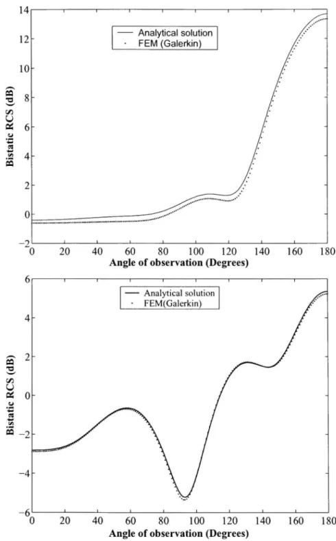
Figure 1.5 Spherical shaped computational domain 38 Figure 1.6 Bistatic Radar Cross Section for k=27r and (p — 0. top : soft
scatterer, bottom : hard scatterer. 41 Figure 2.1 The circular shaped scatterer surrounded with a circular artificial
boundary 65 Figure 2.2 Far-field pattern (between 0 and 45 degrees) of the unit circular
cylinder using the BGT-like ABC 71 Figure 2.3 The elliptical shaped scatterer surrounded with an elliptical, a
circular and a rectangular artificial boundary 75 Figure 2.4 Far-field pattern (between 0 and 180 degrees) of the elliptical
cylinder using the BGT-like and Padé-type ABCs 75 Figure 2.5 Far-field pattern (between 180 and 360 degrees) of the elliptical
cylinder using the BGT-like and Padé-type ABCs 76
Figure 2.6 The submarine-shaped scatterer. 77 Figure 2.7 Far-field pattern (between 0 and 180 degrees) of the
submarine-shaped scatterer using the BGT-like and Padé-type ABCs 79 Figure 2.8 Far-field pattern (between 180 and 360 degrees) of the
Figure 2.9 Mesh of the computational domain bounded by the
submarine-shaped scatterer and the elliptical artificial boundary 80 Figure 2.10 Mesh of the computational domain bounded by the
submarine-shaped scatterer and the rectangular artificial boundary 81 Figure 3.1 The circular shaped scatterer surrounded with a circular artificial
boundary. The computational domain is meshed with structured
quadratic finite éléments 104 Figure 3.2 Radar Cross Section of the sound-hard circular cylinder at ka =
60, O^"'^ = 0 degree, m = 0.15, nx = 1 and n^ = 2 using the
Padé-type ABC 108 Figure 3.3 Radar Cross Section of the sound-soft circular cylinder at ka =
60, 6''"'^ = 0 degree, m = 0.15, nx — 1 and n^ = 2 using the
Padé-type ABC 108 Figure 3.4 Comparison of the computed RCS of the sound-hard elliptical
cylinder at ka = 60, for 0'"'^ = 45 degrees and m = 0.15. We use
the CPWT6 FEM for différent values of n, 112 Figure 3.5 Comparison of the computed RCS of the sound-hard elliptical
cylinder at ka = 60, for 9'"'^ = 45 degrees and m = 0.15. We
again increase the mesh resolution and compare it to the T6 FEM 113 Figure 3.6 Comparison of the computed RCS of the sound-hard elliptical
cylinder at ka = 60, for 0™" = 45 degrees and m = 1.2 114 Figure 3.7 Configuration for the computations : the submarine-like shaped
scatterer is enclosed by an elliptical fictitious boundary S 115 Figure 3.8 Mesh of the computational domain with quadratic finite éléments 115
Figure 3.9 Comparison of the RCS of the sound-hard submarine-like scatterer for kD = 20, m = 1.0 and 9"'^' = 225 degrees using the Padé-type ABC with the T6 and the CPWT6 finite éléments (setting nx == 1 and n, = 5 for the CPWT6 FEM and nx = 2.5
for the T6 FEM) 117 Figure 3.10 Comparison of the RCS of the sound-hard submarine-like
scatterer for kD = 20, m = 1.0 and 6''"'^ = 225 degrees using the Padé-type ABC with the T6 and CPWT6 finite éléments (setting
now nx — 2 and n^ = 3 for the CPWT6 FEM and nx — 3.5 for
the T6 FEM) 118 Figure 3.11 Comparison of the RCS of the sound-hard submarine-like
scatterer for kD = 20, m = 2.0 and 9™" = 225 degrees using the Padé-type ABC with the T6 and CPWT6 FEM {nx = 1 and
a Forme bilinaire symétrique définie sur Hi{Çl) x Hi{Çl)
acLS Forme bilinaire et symétrique associée à la méthode GLS et définie sur i / i ( Q ) X / / i ( f i )
6 Forme linéaire défine sur L2{^)
bcLS Forme linéaire associée à la méthode GLS d Dimension de l'espace (d=l,2 ou 3) k Nombre d'onde
u Champ de pression diffracté Uinc Champ de pression incident h Pas du maillage
nx Nombre d'éléments par longueur d'onde
A forme variationnelle symétrique définie sur H^{Q) x H^{Çl) Bj est une forme variationnelle symétrique définie sur H^{T,) x H^{T,) C est une forme variationnelle symétrique définie sur H^{Ti) x H^{T,) V est une forme variationnelle symétrique définie sur i/^(S) x i/^(S) AG]_S forme variationnelle associée à la méthode GLS
d Vecteur unitaire de direction du champ incident nr Vecteur unitaire normale sortant de îl~ à la frontière F
[A\ Matrice carrée bande, symmetrique, non hermitienne, à coefficients et à
diagonale non dominante
H^{ÇL) Espace de Sobolev définie sur Jl
H^{T.) Espace de Sobolev définie sur E ILU Factorisation incomplète LU
ILUC Factorisation incomplète LU du type Crout [Ke] Matrice rigidité élémentaire
[L] Matrice triangulaire inférieure
[M] Matrice carrée de préconditionnement
[Me] Matrice masse élémentaire \U\ Matrice triangulaire supérieure
DtN Opérateur pseudodifférentiel (Dirichlet to Neumann), relation reliant
l'in-connue physique à sa dérivée normale
Ti. Opérateur différentiel de Helmholtz A -I- A;^
A/, Opérateur différentiel d'ordre i approximant l'opérateur DtN A Opérateur de Laplace
A s Opérateur différentiel de Laplace-Beltrami r Frontière exteme de l'obstacle
Y art Frontière artificielle
« Courbure en un noeud donnée A longueur d'onde
fie Domaine extérieur
Q^"' Domaine extérieure associée kO."
Çl~ Obstacle de frontière F
S Frontière artificielle
T Paramètre de la méthode Galerkin-Moindres Carrés (GLS)
BGT-2 Conditions aux limites absorbantes de Bayliss-Gunzburger-Turkel du se-cond ordre
NRBC Conditions aux limites non-réfléchissantes (Non- Reflecting Boundary Conditions)
La modélisation numérique des problèmes d'ondes demeure un domaine où la recherche est très active depuis près d'un demi-siècle. Cette activité est poussée en partie par l'impor-tance des applications telles que le sonar, le radar, l'exploration géophysique, l'imagerie médicale, les tests non-destructifs et récemment la météorologie. En dépit des progrès réalisés, ce domaine de recherche est toujours considéré comme un des plus difficiles en calcul scientifique notamment lorsqu'il est question d'ondes courtes.
Nous nous intéressons dans ce travail à la résolution des problèmes harmoniques de diff-raction acoustique en milieu infini, régis par l'équation de Helmholtz (ou équation réduite des ondes), avec une condition de radiation à l'infini dite condition de Sommerfeld, par la méthode des éléments finis (MEF). Nous considérons les problèmes directs liés aux applications du type sonar où une onde de pression incidente (harmonique) rentre en in-teraction avec un obstacle donné donnant ainsi naissance à un champ de pression diffracté caractérisé en champ lointain par la section équivalente (ou image) sonar (ou radar) (radar cross section, RCS).
Les premières applications de la technologie MEF se sont concentrées sur les problèmes dits intérieurs (Thompson,2006) où les structures mécaniques ayant une géométrie com-plexe sont couplées de façon directe avec des cavités acoustiques afin soit d'analyser la réponse fréquentielle de telles structures lorsqu'elle sont soumises à des vibrations forcées ou afin d'effectuer une analyse modale pour déterminer les modes résonants.
Toutefois, les énormes progrès réalisés ces dernières années dans le développement de la technologie éléments finis a permis d'étendre ses applications aux problèmes dits ex-térieurs où le domaine d'étude est non-borné. De nombreux travaux démontrant les po-tentialités de la MEF sont publiés régulièrement qu'ils s'agissent de problèmes dits di-rects (Djellouli et (3/.,2000; Tezaur et o/.,2002; Farhat and Hetmaniuk,2002) ou inverses (Farhat et a/.,2002). Des méthodes MEF d'analyse par bandes de fréquences sont
éga-Revue de la littérature et position du problème
La résolution des problèmes extérieurs hautes fréquences demeure un défi pour la MEF standard (Zienkiewicz,2000). En effet, cette méthode exige des ressources de calcul consi-dérables afin de solutionner de tels problèmes notamment lorsqu'il est question d'ondes courtes. A titre d'exemple, résoudre un problème de diffraction acoustique tridimension-nel (Tezaur et a/.,2000) en utilisant des éléments finis quadratiques conduit à la résolution d'un système d'équations à nombres complexes ayant une dizaine de millions d'incon-nues pour un nombre d'onde adimensionnel kD=10 où k est le nombre d'onde et D une dimension caractéristique du sous-marin. Les applications industrielles et militaires re-liées au sonar requièrent la résolution de tels problèmes pour kD beaucoup plus important avoisinant 200 (Gillman,2006). Ceci indique clairement que la méthode des éléments finis standard est incapable d'adresser des problèmes dans la gamme des moyennes et hautes fréquences.
Ainsi, les recherches se sont orientées notamment vers l'amélioration de la technologie éléments finis par entre-autres l'incorporation du comportement ondulatoire de la solu-tion (autrement dit de la nature physique du problème) de ce type de problèmes dans la base d'approximation locale combinée à une décomposition de domaine et une résolution itérative parallèle. Ces améliorations devront permettre d'étendre ses applications à des fréquences encore plus élevées.
Habituellement, pour les moyennes et hautes fréquences, ce sont les méthodes analytiques ou numériques telles que méthodes asymptotiques (Molinet et fl/.,2005), la méthode des conditions de radiation sur le bord (On surface radiation condition, OSRC) (Antoine et al., 1999 ; Antoine et al.,2006) et la méthode des équations intégrales de frontière (Burton and Miller, 1971 ; Colton and Kress,1983 ; Nédélec,2001) qui sont traditionnellement
uti-gueur d'onde en question est du même ordre de grandeur que les dimensions caractérisant l'obstacle. La méthode des conditions de radiation sur le bord bien que rapide par rapport à la méthode des équations intégrales de frontière reste malheureusement dépendante de la forme géométrique de l'obstacle qui doit être convexe.
Harari et Hughes (Harari and Hughes, 1992) montrent que la méthode des éléments fi-nis est compétitive avec la méthode des équations intégrales de frontière standard. En effet, contrairement à la méthode des éléments finis, cette technique est limitée aux pro-blèmes linéaires, isotropes et homogènes. La présence de fréquences de résonances pa-rasites (qui n'ont pas d'origine physique) reliées au problème intérieur associé forcent l'adoption de formulations intégrales, souvent complexes, alternatives telles que celles de Burton-Miller (Burton and Miller, 1971) et la méthode CHIEF (Combined Helmholtz Intégral Equation Formulation) de (Schenck, 1968). Ne nécessitant que la discrétisation des surfaces en 3D, elle conduit, cependant, à des systèmes d'équations denses exigeant ainsi un espace mémoire considérable lorsqu'il s'agit de problèmes 3D où les fréquences en jeu sont relativement élevées. Ces systèmes sont de plus mal-conditionnés compli-quant leur résolution par des méthodes de résolution itératives et augmentant ainsi les temps de calcul. Toutefois, cette compétitivité éléments finis- méthode intégrale devient moins évidente lorsque cette dernière est associée à la méthode rapide des multipôles (Fast Multipole Method, FMM) (Chew et a/.,2001; Darve,2000) et à des solveurs rapides (Darve,2000; Rokhlin,1990; Bruno,2004)
Problématique liée au domaine non-borné
Contrairement à la méthode des équations intégrales de frontière, les méthodes d'approxi-mation par sous domaines telles que la méthode des éléments finis (Zienkiewicz,2000) ou des différences finies (MDF) (Harari and Turkel,1992) sont conçues pour des applications
défi à ces méthodes.
L'application de la MEF ou la MDF nécessite avant tout la définition d'un domaine de calcul borné. Cette opération est réalisée pratiquement en entourant l'obstacle par une frontière artificielle positionnée à une distance, généralement mesurée en multiple de la longueur d'onde correspondant à la fréquence en question (Mittra et a/., 1989), de la sur-face extérieure de l'obstacle.
Le comportement de la solution dans le domaine complémentaire est alors représenté par des conditions aux limites imposées sur la frontière artificielle ou par une interpolation spécifique. La première approche est associée aux conditions non-réfléchissantes ou ab-sorbantes (Givoli,1999; Givoli,2004) alors que la seconde est associée aux éléments infinis (Astley,2000; Gerdes,2000). Pour ces éléments, la précision dépend entre autres du choix des fonctions d'interpolation, leur ordre dans la direction radiale et du choix de la formu-lation variationnelle adoptée (conjuguée ou non). Dans ces deux approches, l'idée est de minimiser les réflexions parasites dues à l'introduction de la frontière artificielle.
Une alternative consiste à remplacer la frontière artificielle par une couche parfaitement adaptée (Bérenger, 1994)(ou Perfectiy Matched Layer, PML) conçue pour amortir toutes les ondes qui y pénètrent. Dans ce cas, la taille du domaine de calcul est élargie par celle de cette couche. L'épaisseur de cette couche peut rapidement accroître l'espace mémoire et les temps de calcul en 3D (Turkel,2007). Cette technique, facile à implémenter dans un code élément fini, semble bien fonctionner en coordonnées cartésiennes et favorise ainsi les couches rectangulaires. Toutefois, la précision des résultats reste sensible à l'amortis-sement (fictif) caractérisant cette couche. De plus. Il n'existe pas à notre connaissance de
Dans toutes ces approches (conditions absorbantes, éléments infinis et couche parfaite-ment adaptée), le problème aux limites reste bien posé au sens de Hadamard et admet ainsi une solution unique.
Conditions absorbantes
non-locales
Les conditions absorbantes peuvent être non-locales comme c'est le cas de la technique Dirichlet à Neumann (Dirichlet to Neumann, DtN) introduite par Keller et Givoli (Keller and Givoli, 1989). Cette technique permet grâce à une expansion en série de Fourier de l'opérateur DtN (opérateur qui relie l'inconnue physique et sa dérivée normale) d'imposer des conditions dites transparentes (sans réflexions) sur des frontières artificielles de formes simples telles qu'un cercle et une ellipse en 2D ou une sphère et une ellipsoïde en 3D (Thompson et a/.,2000). Dans l'implémentation de cette technique, la série de Fourier est tronquée à un ordre m tel que m soit supérieur à kR où R le rayon de la frontière artificielle sans pour autant introduire des fréquences de résonance parasites dans la solution éléments finis (Harari, 1991). L'ordre m peut devenir rapidement trop élevé s'il s'agit de fréquences élevées et/ou de structures allongées.
L'emploi de cette technique conduit à une sous-matrice symétrique mais pleine étant donné que tous les degrés de liberté sur la frontière artificielle sont tous liés entre eux via la condition aux limites DtN. Son stockage peut devenir très vite problématique en 3D lorsque les fréquences en jeu sont élevées. De plus, son utilisation pratique se limite aux frontières de formes circulaire et sphérique, ce qui conduit à de grands domaines de calcul (en termes de longueurs d'onde) lorsqu'il s'agit de problèmes de diffraction mettant en jeu des obstacles de forme allongée. L'implémentation de cette technique dans un solveur
Conditions absorbantes
locales
Alternativement, des conditions locales préservant la structure bande et la symétrie des matrices EF peuvent être construites comme des approximations de l'opérateur DtN (Gi-voli,2004 ; Turkel,2007 ; Tsynkov,1998). Antoine, Barucq et Bendali (Antoine et al.,1999) présentent une procédure générale et rigoureuse d'approximation de l'opérateur DtN, ba-sée sur la théorie des opérateurs pseudodifférentiels, dans le cadre de la méthode des conditions de radiation sur le bord (On surface radiation conditions, OSRC). Cette procé-dure permet de construire des conditions absorbantes d'ordre élevé et donc plus précises. En particulier, elle permet non seulement de retrouver entre-autres les conditions absor-bantes développées par Enquist et Majda (Engquist and Majda,1977), Bayliss et Turkel (Bayliss and Turkel, 1980) et Bayliss, Gunzburger et Turkel (Bayhss et a/., 1982) pour les frontières circulaires et sphériques mais également de généraliser leurs applications à des frontières artificielles de formes générales convexes. Les conditions absorbantes d'ordre supérieur à deux sont rarement utilisées dans la pratique à cause des difficultés liées à leur implementation avec des éléments finis linéaires et quadratiques par d'exemple.
Une étude de comparaison de la précision conditions absorbantes versus éléments infinis a été menée par (Shirron and Babuska,1998) dans le cas du problème de diffraction de la sphère. Celle-ci montre que la précision des résultats obtenus avec les éléments infinis est supérieure à celle avec les conditions absorbantes de Bayliss-Gunzburger-Turkel pour un nombre d'onde adimensionnel égal à kR=10. L'inverse est constatée pour kR=l. Tou-tefois, les systèmes d'équations obtenus en utilisant les éléments infinis sont moins bien conditionnés que ceux avec les conditions absorbantes.
Une altemative prometteuse concernant les conditions absorbantes locales consiste à uti-liser des fonctions auxiliaires pour implémenter les conditions absorbantes d'ordre élevé
Problématique liée au problème de pollution numérique de la MEF
La résolution de l'équation de Helmholtz par la méthode des éléments finis soulève une autre problématique liée à la perte du caractère elliptique de cette équation et sa so-lution fortement oscillante lorsque le nombre d'onde k augmente (Harari, 1991). Ainsi, une dégradation rapide de la précision des résultats éléments finis est constatée à me-sure que le nombre d'onde augmente et ce même si le nombre d'éléments par longueur d'onde est gardé constant (la règle heuristique de dix éléments finis linéaires par lon-gueur d'onde s'avère dans la pratique insuffisante) à l'opposé de la méthode intégrale de frontière (Gerdes,2000). Outre donc l'erreur de discrétisation, il existe une autre erreur désignée dans la référence (Ihlenburg and Babuska,1995) par l'erreur de pollution.
11 est possible de quantifier cette erreur soit par une analyse d'erreur ou de dispersion où l'on montre que le nombre d'onde du système discret k^ diffère du nombre d'onde k du système continu. Ceci se traduit par un retard (un déphasage) entre la solution numérique et la solution exacte. Ihlenburg et Babuska (Ihlenburg and Babuska, 1997) ont montré, pour un problème monodimensionnel que l'erreur relative e de la solution éléments finis hp au sens la semi-norme Hi satisfait pour un kh suffisamment petit : e < Ci(A;h/(2p))P +
C2{kh/{2p))^PkL avec Ci et C2 des constantes indépendantes de k, L désigne la taille
du domaine, h le pas de discrétisation et p l'ordre du polynôme. Le terme Ci{kh/{2p))P représente l'erreur d'approximation qui peut être contrôlée en maintenant le produit kh constant pour un p donné. Le deuxième terme C2{kh/{2p))'^''kL est lié à la pollution. Pour des nombres d'onde adimensionnels kL élevés, l'erreur due à la pollution devient prépondérante et affecte la précision des schémas éléments finis hp standards. 11 est clair aussi qu'on peut contrôler l'effet de pollution soit en utilisant un maillage très fin (kh très petit donc des systèmes d'équations très grands) pour un p fixe, ou au contraire en
Pour les problèmes bidimensionnels et tridimensionnels, la taille du domaine de calcul me-surée en termes de longueur d'onde est dans la pratique importante à cause des contraintes imposées par les conditions absorbantes lorsque les fréquences en jeu sont élevées. En effet, celles-ci sont plus précises lorsqu'elles sont placées suffisamment loin de l'obstacle. La réduction du problème de la pollution numérique implicitement par la réduction de la taille du domaine est donc limitée par cette contrainte. Les remèdes au phénomène de pollution ou de dispersion se sont donc orientés vers la minimisation explicite.
Différentes méthodes ont été développées afin de contrer le phénomène de pollution et stabiliser la méthode de Galerkin ; citons à titre d'exemple : les éléments finis hp (Ih-lenburg and Babuska, 1997), les éléments finis spectraux (Kamiadakis and Sherwin,1999 ; Gary,2002 ; Mehdizadeh and Paraschivoiu,2003), la méthode des éléments finis générali-sés (Ilhenburg,1998) (generalized finite élément method, GFEM ) où l'on retrouve entre-autres la méthode Galerkin-Moindes carrés (Galerkin least- squares, GLS)(Harari,1991) et la méthode des éléments finis quasi-stabilisés (quasi-stabilized finite element)(Babuska and Sauter, 1997)
Dans les revues de littérature récentes de Thompson (Thompson,2006) et de Harari (Ha-rari,2006), sont citées d'autres méthodes de stabilisation telles que la méthode PUFEM (the partition of unity finite élément), la méthode RFB (residual free bubble), la méthode de Galerkin discontinue et enrichie (the discontinuons enrichment methods, DEM), la mé-thode de Galerkin discontinue (the discontinuons Galerkin method, DGM), la mémé-thode de l'élément faible (weak élément method), la méthode variationnelle ultra-faible (ultra weak variational formulation, UWVF) ou récemment la méthode des éléments finis oscil-lants (Gillman et a/.,2007; Gillman,2006) (Oscillated FEM).
comme les méthodes PUFEM et DGM incluent le comportement ondulatoire de la solu-tion dans l'approximasolu-tion locale (au niveau élémentaire) par le biais d'ondes planes ayant des directions spécifiques. Ces méthodes peuvent être regroupées sous le thème des élé-ments finis avec ondes planes (plane wave finite élément, PWFEM).
Problématique liée à la résolution directe et itérative du système discret de Helmholtz
Un autre domaine où la recherche demeure active est celui de la résolution du système d'équations de Helmholtz issu d'une discrétisation par la méthode des éléments finis. En effet, bien que ce système à coefficients complexes, soit linéaire, creux et symétrique (dans le cas où la formulation variationnnelle adoptée est bilinéaire), il est non-Hermitien, à diagonale non-dominante, indéfini et peut être de grande taille.
Les applications pratiques conduisent souvent à plusieurs millions d'inconnues (même en 2D). Les méthodes directes de résolution telles que la méthode d'élimination de Gauss
ou la factorisation LU , bien que robustes en comparaison avec les méthodes itératives,
peuvent devenir excessivement chères en termes de mémoire et temps de calcul dès qu'il s'agit de problèmes tridimensionnels où les fréquences en jeu sont élevées. Générale-ment, la résolution itérative se fait dans l'ensemble des nombres complexes. En effet, la résolution dans l'ensemble des nombres réels bien que possible (Mehdizadeh et Paraschi-voiu,2003), le conditionnement du système à résoudre est mauvais en comparaison avec celui du système original (Zebic, 1992). Dans la pratique, les méthodes itératives de réso-lution utilisées sont celles dites de projection dans l'espace de Krylov (Saad, 1996) telles que GMRES (generalized minimal residual method)(Kechroud et al.,2004), BiCG-Stab (stabilized biconjugate gradient method) (Thompson,2006), et QMR (quasi-minimal resi-dual method) (Thompson et al.,2000). Le choix d'un solveur dépend du problème traité
(Thompson,2006) du moment qu'il n'existe pas de solveur itératif universel pour ce type de problèmes.
Pour accélérer la convergence, ces solveurs sont munis soit de préconditionneurs spéciali-sés dits préconditionneurs analytiques (Gander and Nataf 2001) ou de préconditionneurs algébriques standards à usage général (Kechroud et a/.,2004). Ces derniers sont basés sur les méthodes directes du type factorisation LU, tels que ILUT (décomposition incomplète LU avec seuil) (Saad, 1994) , ILUO ou ILUTC (ILU version Crout) (Li et al.,2002) ou de préconditionneurs modifiés (perturbés) (Mardochée,2001 ) où avant la factorisation in-complète de Cholesky, la partie réelle de la matrice de préconditionnement est modifiée de façon à la rendre moins indéfinie ou définie positive ce qui permet d'accélérer la conver-gence de GMRES. Une autre technique similaire à cette dernière baptisée shifted Laplace
Preconditioners (Erlangga et ai,2004) consiste à construire le préconditionneur à partir
d'un opérateur de Helmholtz modifié en considérant un nombre d'onde complexe. D'autres techniques de résolutions sont basées sur la méthode de décomposition de do-maine (domain décomposition method, DDM), technique qui favorise le traitement para-llèle, avec toutefois la nécessité de stabiliser les problèmes posés dans les sous-domaines. Le solveur FETI-H (Djellouli et a/.,2000; Tezaur et ûf/.,2000) en est un exemple. 11 y a lieu aussi de citer également les méthodes de résolution basées sur les transformations rapides de Fourier (Elman and 0'Leary,1998) et la méthode des domaines fictifs (fictitious do-main method,FDM) (Farhat and Hetmaniuk,2002; Hetmaniuk and Farhat,2003).
Objectifs de la thèse
Nous nous proposons dans cette thèse de solutionner les problèmes de diffraction acous-tique hautes fréquences en milieu non-borné. Notre objectif principal est de développer une méthodologie simple et efficace de résolution itérative de ces problèmes basée sur une méthode de couplage éléments finis (de Lagrange, GLS, et à base d'ondes planes)
-conditions absorbantes généralisées d'ordre élevé basées sur les approximants complexes de Padé. Notre but est d'atteindre des résultats probants aussi bien en champ proche qu'en champ lointain en particulier lors du calcul de la surface équivalente radar ou sonar,(radar cross section, RCS)) qui a un intérêt pratique.
Nos objectifs spécifiques sont dans un premier temps la réduction, pour une précision pra-tique, de la taille du domaine de calcul et des temps de résolution en comparaison avec des méthodologies éléments finis utilisant les conditions généralisées de Bayliss-Gunzburger-Turkel du second ordre, ce qui permet de solutionner des problèmes de fréquences plus élevées pour des ressources de calcul données.
Dans un deuxième temps, notre objectif est une diminution significative de la taille des systèmes d'équations à résoudre par une réduction explicite du phénomène de pollution ceci dans le but d'utiliser des solveurs directs.
Plan de la thèse
La présente thèse s'articule autour de trois chapitres qui ont fait l'objet de publications parues (chapitres 1 et 2) et une soumise (chapitre 3). Trois problématiques sont abordées dans ces chapitres à savoir :
a. La résolution itérative du système discret de Helmholtz par une méthode de pro-jection dans l'espace de Krylov préconditionnée par des préconditionneurs
algé-briques ;
b. Les conditions absorbantes locales généralisées d'ordre élevées ;
c. Les moyens implicite et explicite pour réduire la pollution ou dispersion numérique dans les schémas MEF.
Ainsi au chapitre 1, après une revue de littérature portant sur les conditions absorbantes, nous présentons la discrétisation par la méthode des éléments finis linéaires (schémas de Galerkin et Galerkin-moindres carrés, GLS) du problème de Helmholtz extérieur en 2D et 3D reformulé dans un domaine borné à l'aide des conditions absorbantes de Bayliss-Gunzburger-Turkel d'ordre deux.
Nous développons en particulier une méthode originale de calcul du paramètre r associé à la méthode GLS. Nous étudions par la suite les performances d'une résolution itéra-tive du système d'équations de Helmholtz par la méthode de projection GMRES avec initialisation munie de trois préconditionneurs ILUT, ILUTC et ILUO afin d'en accélérer la convergence. Une comparaison de la précision des schémas de Galerkin et Galerkin moindres carrés est également effectuée.
Au chapitre 2, nous substituons la condition de Bayliss-Gunzburger-Turkel d'ordre 2 par une condition absorbante d'ordre élevé, mieux adaptée aux hautes fréquences, basée sur les approximants complexes de Padé. Le processus de construction de ces conditions à par-tir de l'opérateur DtN est développé. Nous associons ces conditions absorbantes aux sché-mas éléments finis linéaires de Galerkin et Galerkin-moindres carrés pour résoudre itéra-tivement à l'aide du solveur ILUT-GMRES des problèmes 2D de diffraction acoustique hautes fréquences. Nous analysons les performances de cette technique de couplage par rapport à celle utilisant les conditions généralisées de Bayliss-Gunzburger-Turkel d'ordre deux pour différentes formes d'obstacle en particulier le cas où celui-ci est un sous-marin. La solution de ce type problème d'ondes courtes par la MEF nécessite habituellement la résolution d'un système d'équations de plusieurs millions d'inconnus. L'objectif est la ré-duction de la taille du domaine de calcul (et donc implicitement la pollution numérique) et les temps de calcul. Des comparaisons entre la précision des éléments finis linéaires et stabilisés par la technique GLS est menée.
Dans le chapitre 3, nous couplons les conditions absorbantes de Padé, développées dans le chapitre 2, avec des éléments finis quadratiques et des éléments finis quadratiques à base d'ondes planes afin de réduire explicitement le problème de pollution. L'objectif étant cette fois non-seulement la réduction de la taille du domaine de calcul mais également celle du système d'équations de façon à pouvoir le résoudre de manière directe. Ainsi, des problèmes mettant en jeu des fréquences plus élevées que ceux du chapitre deux sont traitées.
Une comparaison éléments finis quadratiques et ceux à base d'ondes planes permet de mettre en évidence outre la convergence hp, la convergence suivant le nombre d'ondes planes par nœud.
Nous terminons cette thèse par une conclusion générale et des recommandations futures. Nous détaillons dans les annexes quelques aspects de mise en oeuvre des techniques pro-posées. Ainsi, dans l'annexe A, nous développons la méthodologie proposée dans le cas 3D. Les résultats relatifs à un obstacle sphérique y sont présentés. Dans l'annexe B, la procédure utilisée pour calculer les poids et les coordonnées des points utilisés lors de l'intégration numérique d'ordre supérieur est détaillée. Enfin, dans l'annexe B, nous pré-sentons de façon succincte le principe de la construction d'un préconditionneur déflaté.
HELMHOLTZ EQUATION BY THE FINITE ELEMENT METHOD
Riyad Kechroud ", Azzeddine Soulaïmani °, Yousef Saad *", Shivaraju Gowdab ° Département de Génie Mecanique,École de Technologie Supérieure,
1100 Notre-Dame Ouest, Montréal,Québec,Canada H3C 1K3
** Department of Computer Science and Engineering, University of Minnesota, 4-192 EE/CS Building, 200 Union Street S.E., Minneapolis, MN 55455, USA This chapter is published as an article in Mathematics and Computers in Simulation
vol.65(2004) pp. 303-321.
In the harmonie régime most diffraction phenomena are govemed by the Helmholtz équa-tion. Propagation/scattering problems are often defined over open (non-bounded) domains and are, as a resuit, solved by the boundary élément method. In this case only the extemal surface is discretized. This leads to Systems of équations of relatively small dimensions which are, however, dense. For 3-D problems in which relatively high frequencies come into play, the required memory and computational resources can quickly exceed those af-forded by available workstations. For thèse reasons and also because integral-based tech-niques are restricted to linear and isotropic problems, the finite élément method is currently enjoying a regain of interest.
The use of the finite élément method requires that we define the boundary of the discretized domain. From a practical point of view, the actual obstacle is surrounded by an artificial boundary, located at a finite distance from the extemal surface. The scattered field out-side the computational domain is thus represented either by boundary conditions known as 'absorbing' (ABC), which are specified on this boundary, or by infinité éléments. In both cases, the idea is to prevent the reflection of waves by the artificial boundary. Bé-renger (BéBé-renger, 1994) proposed to replace the boundary by an absorbing layer, or PML
(Perfectiy Matched Layer), of finite width, whose rôle is precisely to damp the waves dif-fracted by the obstacle. The size of the computational domain is thus increased by the width of the PML.
The technique referred to as DtN (Dirichlet to Neumann), and introduced by Givoli and Keller (Keller and Givoli, 1989), can be viewed as a gênerai procédure for specifying exact boundary conditions, known as 'transparent' (TBC), in the case of artificial boundaries of simple géométrie shapes (circle, ellipse, sphère, ellipsoid). Since the TBC is non local, it leads to couplings between ail degrees of freedom at the artificial boundary, which may entail excessive memory requirements. To overcome thèse difficulties, local absorbing boundary conditions, such as those of Robin, bave been developed. This simple condition is easy to implement but gives poor results.
Enquist and Majda (Enquist and Majda,1977) proposed an approach which consists of ap-proximating the DtN operator. Bayliss and al. (Bayliss et a/., 1982) developed an asymp-totic solution outside the domain to establish thèse conditions. However, the local ABC cannot entirely eliminate the parasitic reflections. On the numerical side, the solution of the Helmholtz équation is particularly diflficult when the frequencies involved are high, because of the loss of the elliptic character, and because of the oscillatory behavior of its solution. The meshes must therefore be very fine in the case of a standard discretiza-tion scheme in order to minimize numerical noise. Spécial discretizadiscretiza-tion schemes, whose implementations are rather involved, hâve been developed to circumvent thèse diflficuhies. The System of équations obtained from the Galerkin discretization scheme is sparse, com-plex and symmetric (but non-Hermitian). It is also generally not diagonal dominant and its Hermitian part is not positive definite.
The itérative method GMRES (Saad and Schultz,1986),combined with an efficient pre-conditioner was found to be fairly robust for solving Systems of this type, especially when the frequencies involved are high. Indeed, direct methods become exceedingly expensive
both in tenus of memory and computations when solving very large size Systems. Indus-trial applications often lead to the solution of Systems of équations of several millions of unknowns. When attempting to couvert this complex System into a real one the number of unknowns doubles, though each of the unknowns is now real and occupies half the space occupied by a complex number What is more serions is the impact on the preconditioner. Converting the complex problem into a real one in the standard way amounts to reordering the complex data and the resulting System becomes more diflficult to precondition. In this case the preconditioned GMRES algorithm converges in a reasonable time only when a full factorization of a Crout type (Zebic, 1992) is performed. This factorization remains ex-pensive. Numerical analysts are currently devoting enormous efforts to develop effective preconditioners. However, their methods hâve had limited success for highly indefinite problems (Mardochée,2001).
In this work we propose to investigate the usefulness of a complex version of ILUT (In-complète LU factorization with Threshold), developed by Saad (Saad, 1994) and ILUTC developed by Li et al. (Li et a/.,2002). Thèse preconditioners are derived from direct so-lution methods. The basic idea is to apply an incomplète factorization of the type LU, with reduced cost, to the original System of équations resulting from the discretization of the Helmholtz équation. Our tests show that thèse preconditioners results in better perfor-mances.
The paper is organized as follows. In the first section we establish the mathematical model which govems acoustic phenomena in d-dimension spaces (d=l,2,3). This model is refor-mulated in a variational form using weighted residuals. Two discretization schemes will be considered, namely the Galerkin and the Galerkin Least-Squares methods. The second section introduces the solution method while section 3 and 4 présent numerical tests and discusses the performance of the solution techniques.
l.I Mathematical model
We are interested in diffraction of an acoustic wave originating from infinity on a bounded obstacle with boundary F. The wave propagates in an open médium Qg- The objective is to develop a model using the finite élément method to deal with problems of acoustic diffraction. First we présent the boundary value problem which govems thèse phenomena in unbounded média. This problem is not adapted to a numerical solution by the finite élément method. It is reformulated by invoking the DtN technique, into another problem which is better adapted to this type of solution. The radiation condition at infinity is thus replaced by a particular boundary condition on an artificial boundary.
l.l.I General model
The d-dimensional (d=l,2,3) problem to solve on the open domain Çlg is as follows (Colton and Kress, 1992): Au + k^u u du or —-on = = =
f
^inc du.nc dn in on on Qe F F (1.1) lim r 2 ( — iku r—.c» drwhere u and / dénote, respectively, the wave diffracted by F and a source function such that / = 0 outside the artificial boundary, which typically assumes respectively a circular (spherical) shape in two (three) dimension problems. The fourth équation of the above problem is the Sommerfeld radiation condition. It guarantees the uniqueness of the solu-tion of this boundary value problem. Only the outgoing waves are therefore allowed and the energy flux is positive.
known function and its normal derivative, on an artificial boundary Tart- This condition denoted by DtN (Dirichlet to Neumann), replaces the radiation condition at infinity. It represents the characteristic impédance outside the computational domain Q. The compu-tational domain Q is then limited intemally by F and extemally by Fart- Denoting by M the DtN operator, the boundary value problem (1.1) can be reformulated as follows :
Au + k^u u du or -;r — on du = = = 0 Uinc OU{jic du in on on
n
F F dn (1.2) = —Mu o n FartIt is known that this boundary value problem admits a unique solution (Zebic, 1992). The exact nonlocal condition introduced by (Keller and Givoli, 1989), translates the fact that the artificial boundary Fart does not yield any artificial reflection. It is therefore a Trans-parent Boundary Condition (TBC) in which Mu can be expressed as an expansion into Hankel flinctions of the first kind. This Hankel séries expansion is obtained from an ana-lytic solution of the Helmholtz équation in the domain outside of Î7. It is limited to an order m such that kR < m, in order to guarantee uniqueness of the solution to the boundary value problem (1.2).
Other methods consist of taking only approximations to the TBC. Thèse conditions are then termed 'absorbing' (ABC). Thus, we do not encounter difficulties inhérent to the non-locality of the TBC. However, artificial reflections on Fart are not avoided. The simplest idea is to impose the Robin condition, namely :
du ^ ^ , T.
This condition, which resembles the Sommerfeld radiation condition, does not perform too well. To reduce reflections on the artificial boundary some authors hâve proposed boun-dary conditions of higher order. Using the framework of pseudo- differential operators, Enquist and Majda (Enquist and Majda, 1977) developed a séquence of local ABCs of in-creasing order. Bayliss and Turkel (Bayliss et a/., 1982) use an asymptotic development in
1/r of the solution u in order to form a séquence of local operators. In two dimensions, The second order Bayliss-Turkel conditions can be written as :
9u _ . u u 1 d'^u
d^~' ~2R^ 8RHI/R - ik) ^ 2(1//? - ik)R'' d9^ ^'^
In 3D, this condition is written as :
More détails on the finite éléments implementations of (4) and (5) can be found in (An-toine and al., 1999 ; Djellouli et al.,2000 ; Tezaur et al.,2000)
I.I.3 Variational formulation
In order to apply the finite élément method, the problem (2) is reformulated in a variational form : Find uin Hi{n) such that :
a{u,v) =b{v)yve Hi(Q) (1.6)
where a is a symmetric bilinear form defined on Hi{Q) x Hi{Q) by :
a{u,v) = / WuVvdÇl - fc^ / uvdQ. + / MuvdF (1.7)
and 6 is a linear form defined on L2{^) by :
It is obvions that when the variational problem (6) is approximated by a finite élément method, the second order Bayliss-Turkel conditions (4) and (5) introduces only additional mass- and stiflfness like matrices defined on F.
In the Galerkin-Least-Squares discretization scheme the variational formulation is adjus-ted in order to account for the residual of the partial differential équation. Under this constraint, the weak form of the équation is :
aGLs{u,v) = bcLsiv) v) with < -Ip aGLs{u,v) = a{u,v) + T
nuHvdn
(1.9)bGLs{u,v) = b{u,v) + T I Hu fdO.
where H is the Helmholtz differential operator 7^(.) = A(.) -I- A;^(.) and r is a parameter whose choice dépends on some design criterion.
1.1.4 Analyti c and Numerical computation of the parameter r
For a regular mesh in two dimensions , consisting of bilinear finite éléments and with a constant mesh size h, the parameter r determined by Harrari et al. (Harari et a/., 1996) is expressed as :
r = i r i - ^ ( : ^ - ^ - ^ - ^ ^ y i with
A;2 V {kh)^2 + f,){2 + fy)
fx = cos {kh cos9), fy = cos {kh sin 9)
where 6 is the direction of propagation of the plane waves. Two values of r corres-ponding to 6 = 0 and to 6 = 22.5 deg. are often used in practice (Harari et a/., 1996; Obérai and Pinsky,2000).
For non regular meshes, we propose as an altemative to compute the parameter r nume-rically. This is donc within each finite élément. The basic idea starts from the System of
équations which arise from the discretized version of the variational formulation above :
[ A ' ] e M e - ( l - T ^ - ' K - ' [ A / ] e M e = { 0 }
where [K]e and [M]e are the élément stiflfness and mass matrices respectively. Multiplying both sides of the above expression by the row vector {u}* = {û}^, the transpose and complex conjugate of u, yields the desired expression for the parameter r :
'\ /L.2
T = ( 1 - T')/k where r ' is given by :
^ ' = T T T ^ F ^ T T T V ^ ' ^ {u}^ = {exp{i(kcos{9)xi + ksm{9)yi))} '^ \ " / e i-'^^J e l^/ e
and X,, yi are the coordinates of the nodes of the élément. It is straightforward to extend this approach to the three-dimensional case and to isoparametric finite éléments.
1.2 Solutio n method
In what follows, we use quadrilatéral finite éléments in 2D and tetrahedral ones in 3D. The discretized version of (6) or (9) resuit in a linear System of équations of the form :
Au = b (1.10)
The coefficient matrix A in the above System, is sparse, symmetric, and complex. Note that it is also non-Hermitian and not diagonally dominant.
As can be seen, the eflfect of the DtN condition in the discretization scheme by standard finite éléments results only in the addition of the complex matrix C to form the global matrix A. In addition, the terms Cij are zéro whenever the nodes with index i or j do not belong to the artificial boundary Fart- If the DtN condition is non-local then clearly the
terms Cij are nonzero for ail nodes of index i, or j belonging to Fart, and this can destroy the band structure of the matrix if a particular numbering is not used.
We exclude the use of direct methods in this study because of their potential excessive cost - especially for 3D problems. Among itérative methods, preconditioned Krylov subspace techniques (Saad, 1996) are the most general-purpose and appear to be a good altemative to direct solvers.
A preconditioned Krylov subspace method for solving the linear system (1.10) consists of an accelerator and a preconditioner (Saad, 1996). In what follows we call M the precondi-tioning matrix, so that, for example, the right-preconditioned System :
AM-^y = b where x = M'^y (1.11)
is solved instead of the original system (1.10). The above system is solved via an "acce-lerator", a term used to include a number of methods of the Krylov subspace class. Thus, a right-preconditioned Krylov subspace method computes an approximate solution from the affine space :
XQ + Span{ro, AA/~Vo, • • • , (vlA/~^)'"~^ ro, } ,
which vérifies certain conditions. For example, the GMRES algorithm (Saad, 1996) re-quires that the residual Vm = b — Axm has a minimal 2-norm.
The most common way to define the preconditioning matrix M is through Incomplète LU factorizations. An ILU factorization is obtained from an approximate Gaussian élimination process. When Gaussian élimination is applied to a sparse matrix A, a large number of nonzero éléments may appear in locations originally occupied by zéro éléments. Thèse fill-ins are often small éléments and may be dropped to obtain Incomplète LU factorizations. Among thèse procédures, is ILU(O) which is obtained by performing the standard LU factorization of A and dropping ail fill-in éléments that are generated during the process.
Thus, the L and U factors hâve the same pattern as the lower and upper triangular parts
of A (respectively). More accurate factorizations denoted by ILU(k) hâve been defined
which drop fill-ins according to their 'levels' in the élimination process, where the levels attempt to reflect size and are defined recursively (Saad, 1996). We will not consider levels other than level zéro in this work.
Another class of preconditioners is based on dropping fill-ins according to their numerical values. One of thèse methods is ILUT (ILU with Threshold). This procédure uses basi-cally a form of Gaussian élimination which générâtes the rows of L and U one by one. Small values are dropped during the élimination, using a parameter droptol. A second pa-rameter, p, is then used to keep the largest p entries in each of the rows of L and U. This procédure is denoted by ILUT {droptol, Ifil) of A. Practical values of Ifil and droptol are Ifil = aNNZ/n, with NNZ the number of non-zero entries of the original matrix, n the number of unknowns, a is a positive integer, and 10~^ < droptol < 10~^. The quotient NNZ/n refers to the average number of nonzero entries in A. - Among other preconditioners we tested, is a complex version of a Crout-based incomplète factorization. A detailed description of this technique is beyond the scope of this article and we refer the reader to (Li et o/.,2002). The method is based on Computing the i-th column of L and the z-th row of U at the i-th step, for z = 1,..., n — 1. There are two attractions of this algorithm. The first is that it présents important advantages in terms of cost, when com-pared with the standard ILUT. A second advantage is that it enables a more elaborate and rigorous dropping strategy which aims at making / — L~^AU~^ small rather than making
A — LU small as is traditionally donc.
AH the incomplète LU factorization techniques bave been developed for cases when the original matrix A has some diagonal dominance properties. The procédures still work for cases when the matrix is not diagonally dominant and this is the main reason why ILU techniques hâve had an excellent success across a broad spectrum of applications. The matrices which arise from the Helmholtz équation can be highly indefinite. In this situation
the resulting incomplète LU factorization can be inaccurate and resuit in an ineflfective preconditioner. We are therefore in a situation where many of the standard techniques can be expected to fail and some of the techniques which are not necessarily compétitive might be useflil. Among thèse we can mention, for example, an approach based on the normal équations :
A"Ax = A"b.
The above system is Hermitian positive definite and can be solved with the conjugate gradient method, preconditioned by a diagonal matrix, or with an incomplète Cholesky factorization. Hère there are two difficulties. The first is that A"A can sometimes be much denser than the original matrix. The second is that positive definiteness does not guarantee the existence of a good-quahty incomplète Cholesky factorization. In gênerai, this approach is not recommended as the condition number of A" A is the square of that of A - so convergence may be slow. Our experiments with this approach hâve not been conclusive so far and will not be reported hère. In essence, the diflficulty is now shiflted to that of preconditioning the matrix A^ A which may be as hard or barder than that of preconditioning the original matrix.
1.3 Numerical Experiments in 2D
Two problems are considered for the numerical experiments in 2D. The first problem is a square domain and is used to study the convergence of ILUT for différent values of
Ifil and drop-tolerance for a well-conditioned problem. For the second problem the
do-main considered is circular and it is used to study the impact of discretization schemes and to study the performance of GMRES for différent frequency régimes and for différent preconditioners. The condition number of the linear system arising from the discretization varies with the number of éléments per wavelength. The analytical solution is available for both the problems and it is used to compute the error in the numerical solution. The com-putations are performed in double précision on Intel Pentium III based PCs (with 512KB
RAM and 600MHz clock speed processor).
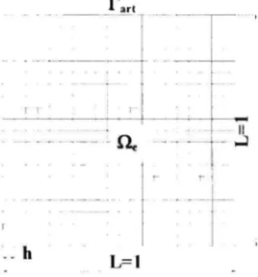
Problem 1.
The problem domain Q is a unit square (Fig.1.1) Q = (0,1) x (0,1). The goveming differential équation is :
( Au + k u = 0 in fie
du .,
-T- +iku dn g in Fa (1.12)
The function g is selected such that the exact solution has the expression : u{x,y) =
exp[ik cos{9)x + k sin(^)y]. The incident angle is set at9 = 45. The domain is discretized
with a structured mesh with a mesh size of h = 1/200. The wavelength is A = 0.628, so the ratio X/h is 125.66. For the solution of the linear system obtained after applying the boundary conditions, the Krylov subspace size is set to 20. The initial guess is zéro and the GMRES itération is stopped when the residual norm is reduced by 10~* or when the number of itérations exceeds 500.
Tari : : ; . : : : : „ : : : : : j j ^ y - : r II 1^1
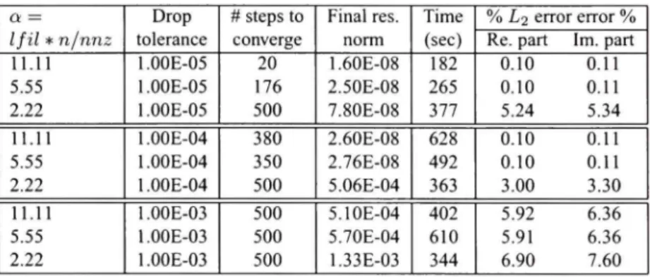
Table 1.1 shows the number of itérations taken by ILUT-GMRES and the error in the computed solution for différent values of Ifil and drop-tolerance. As expected, for this well conditioned Systems, we get the smallest number of itérations for the highest value
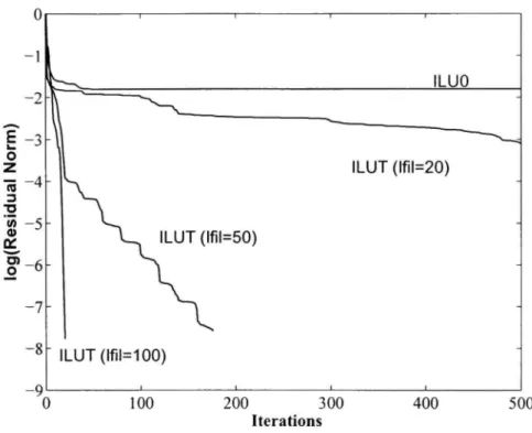
of Ifil and lowest value of drop-tolerance. Figure 1.3 illustrâtes the convergence behavior
of ILUT-GMRES for différent values of Ifil. The results show that as the Ifil is increased the convergence rate increases. It also shows that ILUO stagnâtes.
Table 1.1
Numerical results for problem 1 with ILUT-GMRES
a = Ifil * njnnz 11.11 5.55 2.22 11.11 5.55 2.22 11.11 5.55 2.22 Drop tolérance l.OOE-05 l.OOE-05 l.OOE-05 l.OOE-04 l.OOE-04 l.OOE-04 l.OOE-03 l.OOE-03 l.OOE-03 # steps to converge 20 176 500 380 350 500 500 500 500 Final res. norm 1.60E-08 2.50E-08 7.80E-08 2.60E-08 2.76E-08 5.06E-04 5.10E-04 5.70E-04 1.33E-03 Time (sec) 182 265 377 628 492 363 402 610 344 % L2 error error % Re. part Im. part
0.10 0.11 0.10 0.11 5.24 5.34 0.10 0.11 0.10 0.11 3.00 3.30 5.92 6.36 5.91 6.36 6.90 7.60 Problem 2.
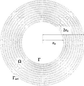
In this problem a soft obstacle, which is a disk of radius ro = 0.5m is considered. The incident wave is plane with a wavelength A, and it propagates along the x-axis. The se-cond order Bayliss-Turkel boundary se-conditions are used on the artificial boundary, located at a distance 2TQ from the obstacle. The discretization uses isoparametric quadrilatéral éléments with 4 nodes (Fig. 1.3). The analytic solution is known and can be found in (Zebic,1992; Bowman,1969).
-9 ILUO ILUT (lfil=20) ILUT (lfil=50) ILUT(lfil=100) 100 200 300 Itérations 400 500
Figure 1.2 Convergence historiés for problem 1 with ILUT-GMRES for différent
values oflfil - residual norms vs itération. 1.3.1 Impac t of discretization
Under the same conditions {k = 2n) and for différent meshes, the accuracy of the results obtained with the GLS scheme are superior to those with the classical Galerkin scheme, see Table 1.2. The number of itérations and exécution times are in both cases almost iden-tical. The Galerkin least-squares scheme leads to a good accuracy even for a rough mesh resolution using 10 points per wavelength. The accuracy of the results is comparable with that obtained in (Zebic, 1992), using a classical Galerkin scheme with an exact non-local Dirichlet to Neumann (DtN) boundary condition. As a comparison, the errors on the real part obtained by Zebic were 5.15,1.33,0.34 for X/h = 10,20,40 respectively. The precon-ditioner selected by Zebic (Zebic, 1992) is based on an incomplète CROUT factorization. In this référence, the finite éléments used are triangles with 3 nodes.