Working paper
(in progress, please do not quote)
The women’s trade-off between work and informal care in Europe
Roméo Fontaine
#, LEDa-LEGOS
May 2010
Abstract
This article focus on the trade-off between work and informal care among women aged 50 to 65. We first specify a simple time allocation model assuming a substitution between the two activities trough the time constraint but also a complementarity trough the agent’s preferences. From the two first-order conditions defining the optimal allocation, we jointly estimate the time devoted to work and care taking into account the simultaneity of the decisions and the censure which characterizes each variable. The model is estimated using data from SHARE, a European multidisciplinary database of micro data on health, socio-economic status and family network. Our empirical results suggest that time devoted to care appears to reduce the working time. In terms of public policy, encouraging the informal care provision for disabled elderly people may then hamper growth in senior employment.
Key words: Long-term care; informal care; female labour supply; time allocation JEL Classification: C34, I12, J14, J22
#Correspondence to: Université Paris-Dauphine, LEDa-LEGOS, Place du Maréchal de Lattre de Tassigny 75775 Paris Cedex 16, France. E-mail : romeo.fontaine@dauphine.fr
1. Introduction
Population ageing is considered in Europe as a major challenge in the coming decades, especially because of the sustainability question of public pensions systems. To contain the dependency ratio, the Stockholm European Council (2001) has set a target for Member States to raise the employment rate to a European average of 67%, setting specific objectives for the senior population. According to the Stockholm European Council conclusions, “it has agreed to set an EU target for increasing the average EU employment rate among older women and men (55-64) to 50 % by 2010”1. This target of 50% was subsequently renewed by the Community Lisbon Program (2005).
In parallel, the growing proportion of elderly in the population is likely to increase the demand for long-term care. To allow the frail elderly to live in the community without excessively increasing public long-term care expenditures, most of the EU members encourage, more or less explicitly, family members to provide care for elderly people.
Considering that senior play a major role in caring for dependent elderly people, it is appropriate to ask whether a policy aimed at extending the work lives of seniors is compatible with a policy aimed at supporting informal care for elderly people. Won’t informal care decrease if the senior employment rate rises? Or, looking at it from the opposite side, won’t shifting the burden of care for elderly people to families hamper growth in senior employment?
Using data from the second wave of the Survey of Health, Ageing and Retirement in Europe (SHARE, 2006-2007)2, figure 1 illustrates at the national level the relationship between the employment rate for women aged 50 to 65 with one living parent3, with the proportion of “intensive” caregivers, defined as those who devote to parental care more than one hour a day or who co-reside with their parent. A decreasing relationship appears between the labour force participation and the provision of informal care. At one end, there are Northern European countries and Switzerland, which present a high employment rate and a low proportion of intensive caregivers. At the other end are the countries of Southeast and Eastern European characterized by a low employment rate and a high proportion of intensive caregivers. Continental European countries lie somewhere in between.
Figure 2 highlights a similar negative correlation at the individual level: the women labour force participation decreases according to the intensity of care provided for a non-coresiding elderly parent. It appears however that women who provide less than an hour a day of care are more frequently employed than no caregivers. This result suggests that the relationship between work and care is not only based on a pure substitution effect between the two activities.
1 In 2001, the European employment rate of this population was 37.7% (Eurostat). 2 See section 5 for a description of the data.
3 We focus in this paper on caregiving provided by children to their parent living without a spouse. Children
Figure 1
Employment rate and proportion of « intensive » caregivers* by country
Austria Germany Netherlands Italy France Denmark Greece Belgium Czech Republic
Poland Sweden Spain Switzerland 0% 10% 20% 30% 40% 50% 60% 70% 0% 5% 10% 15% 20% 25%
proportion of "intensive" caregiver
e m p lo y m e n t ra te
* Women who provide more than one hour a day of care for their elderly parents or who co-reside with him or her. Population: Women aged 50 to 65 and having only one living parent.
Source : Eurostat and SHARE, wave 2 (2006-2007)
Figure 2
Employment rate for women according to the intensity of care
0% 10% 20% 30% 40% 50% 60% 70% nocaregiver ] 0 ; 1 ] ] 1 ; 2 ] ] 2 ; 4 ] ] 4 ; 8 ] ] 8 ; +]
num ber of hours of care per day
e m p lo y m e n t ra te
Population: Women aged 50 to 65 and having only one living parent (women co-residing with their elderly parent are excluded because of lack of information on their caregiving behaviour)
Source : SHARE, wave 2 (2006-2007)
The aim of this paper is to highlight the individual interaction process between working and caregiving behaviour among the senior population. Specifically, the objective is to test the following hypothesis: the provision of informal care encourages individuals to reduce, at least partially, their labour force participation. Previous empirical studies have shows significant differences between men and women behaviours according to the trade-off
between work and care (see, e.g., Carmichael & Charles, 2003). These differences justify an empirical study distinguishing the two subpopulations. The present analysis is restricted to the female population, given that data used do not allow a robust quantitative analysis for the male population4. They are however less likely than women to reduce their working time because of their caregiving role: they are less often involved than women in caregiving for an elderly parent, and among those involved, they devote less time to parental care than women (1 hour and 11 minutes on average against 3 hours and 6 minutes for
women, Fontaine,2009). The female population is then the population for whom the risk of
working time reduction is probably the most important.
The rest of this article is organized as follows. Section 2 summarizes the main results of the empirical literature and discusses econometric methods used. Section 3 presents a simple microeconomic model of the trade-off between labour and care. Section 4 provides the econometric specification. Data used and estimation results are presented in sections 5 and 6. Section 7 presents results of alternative specifications. Finally, section 8 concludes.
2. Survey
Since the mid-90s, several empirical study have analysed in Europe the relationship between labour and caregiving behaviour5. Using a sample of women aged 21 to 59,
Carmichael and Charles (1998) found that in UK, providing less than 20 hours per week of care increase the probability of employment whereas providing more than 20 hours per week of care decreases the labour force participation. Always on UK data, the authors also found that the negative effect of caregiving beyond a certain threshold would be lower for men than for women and that the negative effect on employment is greater for those caring for someone living in the same household (Carmichael& Charles, 2003). More recently,
Heitmueller (2007) confirmed these results in the English case: providing more than 20 hours per week of care for someone living outside the household and caring for someone living in the same household negatively impact the labour force participation.
To our knowledge, only three studies based outside of UK analyse in Europe the effect of caregiving on the labour behaviour. Crespo(2007), using data from the first wave of SHARE (2004) found that in Northern and Southern European countries, the caregiving provision on a daily basis reduces women labour force participation6. Bolin et al. (2008), using also data from the first wave of SHARE but through a different econometric approach, found that caring for an elderly parent has a negative effect on labour market partipation only for men living in Continental European countries. Finally, Casado-Marín et al. (2008) exploited data from the European Community Panel Data. Their results suggest that among employed women, becoming caregiver do not affect labour outcome whatever the group of countries considered. In contrast, for women who were not working prior to becoming a caregiver, the
4 Among the 1037 men aged 50 to 65 included in our sample, only 46 provide on average more than an hour a day of care for their elderly parent. Moreover, only five of the thirteen countries in the survey are characterized by a sample including more than two men providing more than an hour per day of care.
5 See Ettner (1995, 1996), Johson & Lo Sasso (2000), Pezzin & Schone (1999), Stern (1995) and Wolf & Soldo (1994) for previous works on US data. See also Berecki-Gisolf et al (2008) for a study using an Australian database. 6 The author does not test the effect for European continental countries.
probability of entering employment decreases significantly in Southern and Continental European countries.
All these studies highlight a statistically significant relationship between care and employment, even if results differ according to the terms of the relationship and the countries concerned. All of them focus on the causality from caregiving behaviour to labour behaviour. In other words, they analyse the causal effect of an exogenous variation of caregiving (explanatory variable) on a given labour outcome (dependent variable). In this context, the gross negative correlation between labour and caregiving outcome comes from the negative effect of caregiving on the propensity to work.
The main issue of the empirical analysis is the potential endogeneity of the caregiving behaviour. Indeed, the labour behaviour may be considered as determinant of the caregiving one and not the reverse. The gross negative correlation between work and caregiving could then be explained by the fact that being unemployed favours the provision of informal care, since non-workers generally facing lower opportunity costs than workers. From this point of view, individuals who retired before the question of providing care for an elderly parent arises are not concerned by the effect of caregiving on labour force participation: their labour supply will be equal to zero whatever their caregiving behaviour. However, the fact that non-workers are more often caregivers than workers may confuse the empirical analysis because it leads to a negative correlation between care and work that could be wrongly interpreted as a negative effect of caregiving on labour supply.
To control the endogeneity of caregiving, three methods have been identified in the litterature.
Casado-Marín et al. (2008) and Berecki-Gisolf et al. (2008) have used longitudinal data and test the effect of caregiving on the probability of working in wave 2 only on individuals in employment in wave 1. Excluding from the empirical analysis individuals who were out the labour market in wave 1 allows not to take into account those for whom the causal relationship may go from the labour behaviour to the caregiving one. The longitudinal dimension of SHARE allows to apply this approach. However, it will not be used in this article because it only reduces the endogeneity problem without really addressing it. Indeed, we may expect that, due to their inactivity, individuals who left the labour market between the two waves are more likely to become caregiver. For them, the labour behaviour determinates the caregiving behaviour and not the reverse.
Bolin et al. (2008), Ettner (1995, 1996) or Heitmueller (2007) have used an IV approach. The objective is to consider in the caregiving behaviour only the component which can not be explained by the labour behaviour. The parent’s level of disability could capture this dimension and thus be qualified as a good instrument since it can be assumed that it affects labour behaviour exclusively through its effects on caregiving behaviour. From this point of view, the SHARE survey supplies a limited number of instruments. Those used by Bolin et al. (2008), from the first wave of SHARE have a low explanatory power for caregiving and even some may be strongly suspected of endogeneity (e.g. the geographical proximity between the child and his or her parent).
A third method, that we will explore here, is to jointly estimate the labour supply and care provision. Crespo (2007) and Johnson & La Sasso (2000) adopt this type of specification. They allow the caregiving supply to be a determinant of the labour supply but do not allow
the reversal causality, i.e. they do not consider the labour supply as an explanatory variable of caregiving. Then, they focus only on the effect of caregeving behaviour on working behaviour, leaving the opposite effect aside.
To study the trade-off between working time and caregiving time, we estimate here a bivariate tobit model. The estimated model matches the two first order conditions of a microeconomic model in which the time devoted to work and care are endogenous and jointly determined. Therefore and contrary to bivariate models of Crespo (2007) and
Johnson et La Sasso (2000), the estimated model will allows to simultaneously estimate the two reciprocal causality.
3. Microeconomic Framework
The trade-off between working time and caregiving time involves different mechanisms. The
substitution effect is the most frequently mentioned in the literature (see e.g.
Carmichaeland Charles, 1998, Johnson and La Sasso,
2000).
It comes from the time constraint: by devoting increasing time to a given activity, the agent is constraint to reduce the time available for other activities. Through this, working time and caregiving time appear as substitute.However, both activities may on the contrary be considered as complementary due to agent preferences. Three effects may occur. The first one is the “respite effect” (Carmichael& Charles,1998). It illustrates the fact that working may offer to the caregiver a way of freeing oneself from the emotional demands associated with the care provided for a relative. The second one is the “protection effect”. Using results from a qualitative survey conducted in
France among women providing support to their elderly parent, Le Bihan and Martin (2006)
suggests that working is a protective activity for the caregivers. It allows them not to totally be absorbed by their caregiver activity. Unemployed individuals could therefore have a lower propensity to provide informal care for fear of not being able to limit their involvement, as the needs of the elderly parent increase. The third effect is the “productivity effect”: some occupations may allow the development of know-how that can be used in caregiving (personal care for a nurse, help with paperwork for bank employee). In this case, working tends to increase the propensity to provide informal care. Through these three effects, the two activities, i.e. working and caring, appear as complement. To the best of our knowledge, they have never been integrated within a microeconomic model.
To sum up, we may assume that the relationship between working time and caregiving time depends on two opposite mechanisms: a “substitution effect” which comes from the time
constraint and a “complementarityeffect” which comes from the agent preferences.
To formalize these two mechanisms, we consider a simple time allocation model. The child (say a daughter), decides to allocate her time between paid work T, care Aand leisure L. We assume the daughter is characterized by a utility function U :
(
C,L,V(A,A ,S))
U
U= o (1) The utility function depends on the private consumption of a composite commodity C , the amount of leisure L and the parent’s (say a mother) well-being V . We also assume that the
mother’s utility function V depends on care provided by her daughter A , on care provided by others sources Ao and on parental health status H . Care provided by others sources and
parent health status are supposed to be exogenous.
The amount of care provided by the daughter A is chosen by the altruistic daughter, the mother adopting a passive behaviour. The daughter maximizes her utility function subject to two constraints: C≤wT+R (2) 1 ≤ + +L A T (3) where w is the daughter’s wageand R the daughter’s exogenous non labour income. For convenience, the price of the composite commodity has been normalized to one. Constraint
(2)states that consumption can not exceed the financial resources of the daughter. The constraint(3) ensures that time allocated to work, care and leisure can not exceed the total amount of time, normalized to one.
We assume that the level of satisfaction of the daughter and mother are increasing in each argument(UC >0,UL >0,UV >0,VA >0,VAO >0andVH >0),thatUandVarecontinuous,
twice differentiable and quasi-concave(UCC <0,ULL<0,UVV <0,VAA<0,VAOAO <0,VHH <0)7.
We finally assume that the “complementarity effect” leads the caregiving marginal utility to positively depend on working time:
U
AT=
∂
U
A∂
T
>
0
, with UA=UV.VA.Hence, the first-order conditions which give the optimal time allocation are:
w U U C L = (4) L A U U = (5)
The equilibrium condition (4) is identical to the standard labour supply model in which workers allocate their time only between work and leisure. Under this condition, workers increase their working time as long as the value of an additional hour of work (wUC) is higher than the marginal utility of leisure (UL). Some individuals may nevertheless prefer
not to work if they are characterized by a reservation wage which exceeds the real wage, i.e. if only negative values of working time are solution of the first-order condition (4). By defining T* as the propensity to work (the value of working time which is solution of the first-order condition (4)) and Toptas the optimal working time, we can specify from this condition a function Topt(A)=max(T*(A),0) which associate for each possible caregiving time the optimal working time. Trough this function, the impact of an exogenous positive variation of A on T* is given by:
CC LL LL T U w U U ² + − = α < 0
(6)
Given the assumption made, this expression is strictly negative: the propensity to work depends negatively on caregiving time. Hence, all exogenous chocks that increase the time
7 Following Johnson and La Sasso (2000),we also assume that =0
CL
devoted to care reduces workers’ labour supply while it reduces the non-workers’ incentive to enter employment.
According to the equilibrium condition (5), an individual allocate his time so that the marginal utility of caregiving is equal to the marginal utility of leisure. A corner solution is also possible here if the value of the first hour devoted to parental care does not offset the utility lost of reducing leisure time. As previously, by defining A* as the propensity to provide parental care (the value of caregiving time which is solution of the first-order condition (5)) and Aoptas the optimal caregiving time, we can specify from this condition a function Aopt(T)=max(A*(T),0) which associate for each possible paid working time the optimal time devoted to parental care. Trough this function, the impact of an exogenous positive variation of T on A* is given by:
AA LL AT AA LL LL A U U U U U U + − + + − = α (7)
The sign of this expression is indeterminate. It depends on the relative magnitude of the
substitution effect (−ULL (ULL+UAA)<0
)
and the complementarity effect(−UAT (ULL+UAA)>0).
The ambiguity about the effect of an exogenous variation of working time on time devoted to parental care disappears ifwe assume, following Johnson and La Sasso (2000), that the relationship between working time and caregiving time is solely based on the time constraint, that is if UAT =0. Then, the model predicts a strictly negative relationship between the two activities. This prediction is however not robust empirically: all thing being equal, a number of empirical studies cited above draw to the conclusion that the two activities are not significantly interrelated. Carmichael and Charles (1998) even found that women who provide less than 20 hours per week of care are more likely to work than noncaregivers. Fontaine (2009), using data from SHARE, find a similar result. Hence, it seems relevant to assume the existence of a trade-off mechanism leading to the complementarity of both activities.
To investigate the effects of some different exogenous variables on the optimal time allocation, the first-order conditions and the blinding constraints are completely differentiated. Some comparative statistics from the model are presented in equations (8)-(13) below (for individuals characterized by an interior solution):
0 ) ( . 1 < + = CC AA LL opt U U wU D dR dT (8) ) ( . 1 AT LL CC opt U U wU D dR dA + − = (9) 0 . 1 0 0 > − = AA LL opt U U D dA dT (10) 0 ) ( . 1 0 0 < + = AA CC LL opt U wU U D dA dA (11) 0 . 1 > − = AH LL opt U U D dH dT (12) 0 ) ( . 1 + < = AH CC LL opt U wU U D dH dA (13)
where D=ULL(UAT −UAA)−w²UCC(UAA+ULL) <0
0 0 V AA
AA U V
U = , with the assumption that 0
0 < AA U AH V AH U V
U = , with the assumption that UAH <0
According to the equations (8)-(9), a positive shock on the non labour income decreases hours of paid work because the consumption increase reduces the marginal utility of consumption, which in turn reduces the value of an additional hour of work. The effect on
time devoted to care is however ambiguous. It depends on the sign of αA
,
which measuresthe effect of an exogenous variation of working time on the propensity to care. If the substitution effect is greater (in absolute value) than the complementarity effect (αA <0 or similarly ULL+UAT <0
)
, a positive shock on the non labour income increases caregiving time. On the contrary, if the substitution effect is lower (in absolute value) than the complementarity effect, a positive shock on the non labour income will decrease time devoted to parental care. As expected, equations (10)-(13) indicate that when alternative sources of caregiving are available to the parent, such as care provided by others relatives or professional care, or when parent is in better health, individuals devote less time to care and more time to paid work.To summarize the main predictions of our microeconomic framework, we expect that all shocks increasing time devoted to care lead to a decrease in time devoted to paid work. On the contrary, the model does not allow to predict how an exogenous shock on time devoted to paid work affects time devoted to parental care. Whether positive or negative, we may however expect the effect to be modest if the two opposite effects, i.e. the substitution effect and complementarity effect, are of similar magnitude.
4. Estimation strategy
In order to empirically address the trade-off between labour and informal care, we estimate from the two previous first-order conditions a simultaneous equations model taking into account that working and caregiving time are mutually dependent and left-censored at 0. Assuming linear specifications, we estimate the following bivariate-tobit model (Amemiya,1974): Model A > = otherwise if 0 0 * * i i opt i T T T et > = otherwise if 0 0 * * i i opt i A A A (14) with + + + = + + + = Ai opt i A Ai A i A i Ti opt i T Ti T i T i u T x x A u A x x T α β δ α β δ * *
where xTi (resp.xAi) and uTi (resp. uAi) capture the observable and unobservable
exogenous explanatory variables of time devoted to paid work (resp. parental care) and xi
the set of explanatory affecting both the working and caregiving time. The first equation ( Ti =δTxi+βTxTi+αTAiopt+uTi
*
)
results from the first-order condition(4)
which determines the optimal working time conditionally on caregiving time. With regard to the previous microeconomic framework, the expected sign of α1 is negative. The second equation ( Ai* =δAxi+βAxAi +αATiopt +u ) results from the first-order condition(5) which determines the optimal caregiving time conditionally on working time. Our theoretical framework does not allow to predict the sign of α2. Considering simultaneously, both
equations specify the optimal time allocation ( iopt opt
i A
T , ) in the meaning that they define a situation in which the individual has no incentive to deviate. In such a situation, the working time is optimal given caregiving time, while caregiving time is optimal given working time.
Model Ais similar to the model proposed byAmemiya (1974) because we assume that each
dependent variable is a function of the other observed dependent variable. It thus differs from the model proposed by Nelson and Olson (1978)where each dependent variable is a function of the other latent dependent variable. The choice of one or the other specification is not neutral. It depends on whether the theoretical economic model itself is simultaneous in the latent or observed dependent variables (Blundelland Smith, 1994). In the model proposed by Amemiya (1974), the censoring mechanism acts as a constraint on agent’s behaviour, whereas in the model proposed by Nelson and Olson (1978) the censoring mechanism acts as a constraint on the information available to the econometrician but not on the agent’s behaviour itself. Choosing the model A, we assume, according to the previous theoretical model, that censoring mechanism affects the agent’s decision making process. In others words, we consider for example that two non-workers, one characterized by a reservation wage slightly higher than the real wage and the other characterized by a reservation wage much higher than the real wage, will provide the same amount of care all things being equals.
Unlike the model proposed byNelson and Olson (1978),model Amay nevertheless present a
risk of incompleteness in the sense that, for a given vector of exogenous variables (both observed and unobserved) it does not always predict a unique time allocation. This incompleteness stems from the fact thatmodel A defines the optimal allocation as the intersection of two non linear functions, one giving the optimal working time as function of caregiving time and the other giving the optimal caregiving time as function of working time. As illustrated by figure 3, this non linearity may potentially leads to several intersection points. In this case, the model predicts multiple equilibria. To overcome this difficulty, we impose prior to estimating the model the “coherence condition” (Maddala 1983, Amemiya, 1974, Gourierouxet al.,1980):
0 .
1−αAαT > (15)
This condition ensures the completeness of the model whatever the individual characteristics (observed and unobserved). As suggested by Maddala (1983), this constraint can legitimately be imposed whenever a theoretical justification permits it. Here,
conditionally on the assumptions made about the agent’s preferences, the coherence condition appears to be respected. From the expressions (7)-(8), we indeed obtain:
0 ) ).( ( 1 2 > + + − = − AA LL CC LL T A U U U w U D α α (16)
Imposing this condition, with regard to our microeconomic framework, is thus absolutely not restrictive. In the section 7, we partially loosen this constraint by adding to the model a selection rule which allows to select a specific equilibrium in case of multiple equilibria (Krauth, 2006). Results are similar because the model still converges to a situation without multiple equilibria.
Figure 3: illustration of a situation with multiple equilibria
Let
(
( , ) ( , iopt))
opt i i i A T A TP = denoted the probability for a given allocation to be optimal for the
individual i . For positive value of Ti and Ai, we have:
(
)
(
Ti i T i T Ti T i Ai i A i A Ai A i)
opt i opt i i i A T A P u T x x A u A x x T T P ( , )=( , ) = = −δ −β −α , = −δ −β −α (17)(
)
(
Ti i T i T Ti Ai A i A Ai A i)
opt i opt i i T A P u T x x u x x T T P ( ,0)=( , ) = = −δ −β , <−δ −β −α (18)(
)
(
Ti T i T Ti T i Ai i A i A Ai)
opt i opt i i T A P u x x A u A x x A P (0, )=( , ) = <−δ −β −α , = −δ −β (19)(
)
(
Ti T i T Ti Ai A i A Ai)
opt i opt i A P u x x u x x T P (0,0)=( , ) = <−δ −β , <−δ −β (20) αT 1/αA ) max( ) , 0 max( ' ' Ai opt i A Ai A opt i Ti opt i T Ti T opt i u T x A u A x T + + = + + = α β α βWe assume that the residuals are distributed according to a bivariate normal density function: (uTi,uAi)~N(0,0,σT,σA,ρ). Hence, the previous probabilities may be expressed as
following:
(
)
(
A T)
(
i T i T Ti T i i A i A Ai A i)
opt i opt i i i A T A f T x x A A x x T T P( , )=( , ) = 1−α .α −δ −β −α , −δ −β −α (21)(
)
∫
− − −(
)
∞ − − − = = Axi AxAi ATi Ai Ai Ti T i T i opt i i i A T f T x x u du T P( , ) ( ,0) δ β α δ β , . (22)(
)
∫
− − −(
)
∞ − − − = = Txi TxTi TAi Ti Ai A i A i Ti opt i i i A A f u A x x du T P( , ) (0, ) δ β α , δ β . (23)(
)
(
)
Ai x x x x Ti Ai Ti i i A f u u du du T P∫
− Ai− AAi∫
T i T Ti ∞ − − − ∞ − = = ' ' . , ) 0 , 0 ( ) , ( δ β δ β (24)where f is the joint density function of the bivariate normal.
The model can then be estimated with the maximum likelihood method, under the following constraint: 1−αA.αT >0.
5. Data
To estimate the model, we use the second wave (2006-2007) of the Survey of Health, Ageing and Retirement in Europe (SHARE). SHARE follows the design of the US Health and Retirement Study (HRS) and the English Longitudinal Study of Ageing (ELSA). It is a multidisciplinary database of micro data on health, socio-economic status and social and family networks of more than 30 000 individuals aged 50 or over.
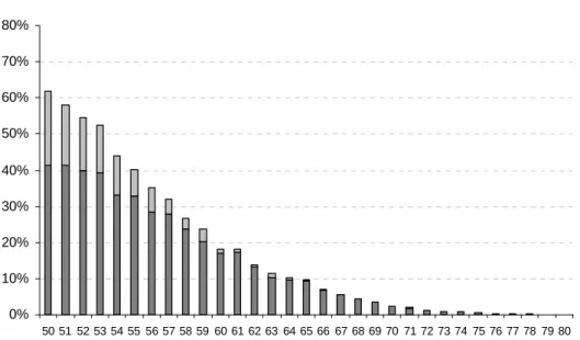
For the purpose of this study, we restricted the sample to women because very few men provide “intensive” care and because of considerable evidence suggesting that female labour supply is relatively elastic (Pezzin and Schones, 1999). We have only considered women aged 50 to 65, not only because, over 65, the probability to work is close to zero, but also because the proportion of those having at least one living parent is very low (table 4).
We focus the analysis on care provided by daughter for their parent. Alternatively, we could have focused on care provided by individuals to their dependent spouse but adverse effects on labour behaviour are less expected given that it generally concerns elder caregivers who are already retired. As previously mentioned, we also restricted the sample to respondents having a single living parent8. Finally, to restrict the analysis to women having the opportunity to provide care for their parent, we selected respondent who have described their parent’s health status as “fair” or “poor”9.
8 See Fontaine et al. (2007) for a comparison of children’s caregiving behaviour in the presence of a spouse. 9 The respondent might choose between five terms to describe their parent’s health status: “excellent”, “very good”,
Figure 4: Proportion by age of women having at least one living parent 0% 10% 20% 30% 40% 50% 60% 70% 80% 50 51 52 53 54 55 56 57 58 59 60 61 62 63 64 65 66 67 68 69 70 71 72 73 74 75 76 77 78 79 80 age
one living parent two living parents
To sum up, our sample includes women aged 50 to 65, having one living parent whose health status is seen by his or her daughter as “fair” or “poor”. Moreover, because of a lack of information on intra-household caregiving we had to exclude daughter living with their elderly parent. The final sample includes 1325 observations.
The dependent variables of the model are the number of hours worked a week and the number of hours a week devoted to parental care. 38% of women in the sample are employed and 37% provide care for their elderly parent (table 1).
Table 1: Worker and caregiver distribution Caregiver 0 1 0 547 (41%) 278 (21%) 825 (62%) Worker 1 296 (22%) 204 (16%) 500 (38%) 843 (63%) 482 (37%) 1325 (100%)
The optimal time allocation is assumed to depend on three groups of variables. The first corresponds to the daughter’s socio-demographic characteristics. Our empirical model includes the following variables: age, education level, marital status, number of children, health status and the non labour income. We do not use the wages as explanatory variable even if the information is available for workers. As emphasized by Ettner (1995), the imputation of wage rates for non workers involves identification issues because the variables that influence the potential wage rate are likely to directly impact the choice of work hours.
Following Ettner (1995) and Dimova & Wolff (2010), we therefore include determinants of wage rate in the working time equation, such as age or education level, rather than the wage itself.
The second group of variables corresponds to the parent’s characteristics. In the model, we control for the parent’s gender, age and health but also for the geographical proximity between the daughter and her parent. To measure the parental health status we only have a variable indicating how the daughter appreciates the general health status of her parent. In particular, no information is available on the parent’s incapacity level, even though it may be partially captured by the parent’s age variable. Moreover, we do not know if the parent lives in the community or in a nursing home and if he or she receives formal care. This lack of information may lead to a negative coefficient correlation between the residuals of the two equations if, for instance, professional care (in institution or in the community) encourages daughter to increase her working time (to finance the professional care) and reduces the caregiving time.
Finally, the third group of explanatory variables corresponds to the siblings’ characteristics. The model includes as explanatory variables the number of brothers, the number or daughters and the birth rank of the respondent. We distinguish the number of siblings according to their gender in order to take into account that daughters are more likely to provide care than sons.
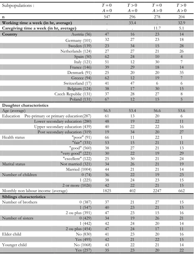
Table 2 reports the distribution of the working and caregiving behaviour conditionally on the exogenous variables.
Table 2: Working and caregiving behaviour according to the exogenous variables In %
Subpopulations :
T=0 0 = A 0 > T 0 = A 0 = T 0 > A 0 > T 0 > A n 547 296 278 204Working time a week (in hr, average) . 33.4 . 32.9
Caregiving time a week (in hr, average) . . 11.7 5.1
Country Austria (56) 47 16 23 14 Germany (101) 32 27 23 18 Sweden (139) 23 34 15 28 Netherlands (124) 27 27 21 26 Spain (50) 62 24 10 4 Italy (121) 51 12 30 7 France (146) 39 29 18 14 Denmark (91) 25 20 20 35 Greece (94) 62 12 19 7 Switzerland (17) 41 47 6 6 Belgium (124) 38 17 30 15 Czech Republic (131) 37 28 27 8 Poland (131) 67 12 15 5 Daughter characteristics Age (average) 56.5 53.4 56.6 53.6
Education Pre-primary or primary education(287) 61 13 20 6
Lower secondary education (280) 48 19 22 11
Upper secondary education (439) 40 22 22 16
Post secondary education (319) 19 34 20 27
Health status "poor" (91) 66 11 22 1
"fair" (331) 53 15 21 11
"good" (560) 38 27 21 13
"very good" (221) 30 22 19 29
"excellent" (122) 25 30 21 24
Marital status Not married (321) 34 26 21 19
Married (1004) 44 21 21 14
Number of children 0 (74) 36 22 19 23
1 (225) 38 24 23 15
2 or more (1026) 42 22 21 15
Monthly non labour income (average) 1825 402 2247 662
Siblings characteristics Number of brothers 0 (387) 37 21 27 15 1 (547) 40 23 21 15 2 ou plus (391) 47 23 15 16 Number of sisters 0 (429) 34 19 26 21 1 (442) 42 24 20 14 2 ou plus (454) 47 24 17 11 Elder child No (830) 41 23 20 16 Yes (495) 42 21 22 15 Younger child No (1068) 43 22 21 14 Yes (257) 35 23 20 22 Continued…
Continued… 0 = T 0 = A 0 > T 0 = A 0 = T 0 > A 0 > T 0 > A Parent characteristics Gender Woman (1154) 41 22 21 16 Man (171) 44 27 18 11 Age (average) 85.0 82.6 85.8 84.8
Health status "fair" (795) 39 26 19 16
"poor" (530) 45 17 24 14
Proximity In the same building (58) 36 21 31 12
Less than 1 km away (191) 34 10 36 20
Between 1 and 5 km away (246) 41 14 26 19
Between 2 and 25 km away (344) 41 24 19 16
Between 25 and 100 km away (225) 42 28 16 15
Between 100 and 500 km away (161) 47 30 12 11
More than 500 km away (48) 63 23 10 4
More than 500 km away in another country (52) 42 46 6 6
In brackets, the number of individuals in the sample.
6. Results
Although the censure characterizing the working and caregiving time allow to identify the parameters of the model even if we include the same explanatory variables in each equation, we have also imposed some exclusion restrictions. First, we assumed that the siblings and parent’s characteristics do not impact the working time conditionally on the caregiving time. Siblings and parent’s characteristics are likely to affect the education level of each child and then their labour supply (Bommier and Lambert, 2004; Picard and Wolff, 2010). However, this effect is here controlled by the inclusion in the working time equation of the education level. Second, we assumed that the individual characteristics available here do not impact the caregiving decision conditionally on the labour behaviour. This assumption is based on previous empirical results showing that the probability to provide care or the quantity of care provided are not associated with child characteristics (see for instance Byrne et al., 2009).
In order to test the validity of these exclusion restrictions, we have first estimated an unrestricted model including the same set of explanatory variables in the two equations (see annexe 1). Results show that the exclusion restrictions are relevant. Conditionally on the caregiving time, siblings and parent’s characteristics do not impact the propensity to work whereas, conditionally on the working time, the time devoted to care does not appear significantly associated with the individual characteristic of the daughter, except for the positive effect of her non labour income.
Columns (1)-(2) of table 3 report our estimation results.
As expected, the working time is negatively associated with the age and the non labour income but positively associated with the education level (column 1 of table 3). With regard to family network, being in couple significantly reduces the labour supply whereas the variable the number of children is not significant. Moreover, the propensity to work is
influenced by the individual health status. Women declaring a “fair” or a “poor” health present a lower propensity to work. Note that this variable may suffer from an endogeneity bias since we do not control for the reversal causality, i.e. the impact of working behaviour on health status. Results remains however unchanged when we remove this variable from the estimation.
Column (2) of table 3 reports the estimation results for the caregiving time equation. As previously mentioned, the propensity to provide care appears not significantly associated with the individual characteristics expect for the non labour income which positively impacts caregiving time. The care provision is however influenced by the siblings’ characteristics. As expected, the number of brothers and number of sisters do not have the same impact on the caregiving behaviour: having a sister has a significant negative impact on the propensity to provide care whereas having a brother has a negative but not significant impact. In particular, women having only brothers seem to adopt the same caregiving behaviour as those with no siblings. Furthermore, being the elder child increases the propensity to provide care. The number of siblings and birth rank effects may reveal the existence of contextual interactions if the siblings’ characteristics (regardless their care provision) directly influence individual caregiving behaviour, but may also reveal the presence of endogenous interactions, if the siblings’ characteristics act as proxies of the siblings’ care provision (Manski, 2000). The model is however unable to disentangle this two mechanisms. Furthermore, being the eldest child increases the propensity to provide care Regardless the parent’s characteristics, our estimation provides consistent results with the existing literature. In particular, the daughter’s care provision depends positively on the parent’s age and negatively on the parent’s health status. Our results also indicate that mothers receive significantly more informal care from their daughter than father10 and that children living further away from their parents are characterized by a lower propensity to care than closer children11.
Turning now to the trade-off between care and work, estimations results appear consistent with our a priori expectations. More precisely, our results suggest that the care provision has a significant negative impact on the propensity to work (α)T =−1,78***) whereas the time spent working has a significant positive impact on the propensity to provide care
**) * 53 . 0
(α)A = . With regard to our microeconomic framework, this last result confirms the existence of the complementarity effect and shows that it dominates the substitution effect.
10 In their structural model, Byrne et al. (2009) identify three mechanisms for the gender’s parent to influence the care provision. Every things being equal, mothers and fathers may differ according to (i) health status, (ii) the burden associated with the care provision and finally, (iii) the effectiveness of the care provision. Their results provide some evidence that (i) fathers experience significantly greater health status than mothers (daughter’s caregiving marginal utility is thus higher when she provides care for her mother rather her father), (ii) care provided for mothers is less burdensome than care provide for fathers and (iii) care provided for mothers is less effective than care provide for fathers.
11 The fact that geographical proximity could be endogenous was examined by Stern (1995). The endogeneity bias appears very limited.
Table 3: Estimated coefficients
not constraint model model with
α
A=
0
model withα
T=
0
(1) * T (2) * A (3) * T (4) * A (5) * T (6) * A Constant 29.93*** (5.32) -5.98* (3.53) 27.76*** (4.84) 5.29 (3.37) 20.02*** (6.19) 1.00 (3.11)
Country dummies Yes Yes Yes Yes Yes Yes
Daughter characteristics
Age 50-51 Ref. Ref. Ref. Ref. Ref. Ref.
52-53 -1.51 (2.98) . -0.51 (2.72) -0.47 (1.70) -1.40 (2.69) . 54-55 -10.61*** (3.15) . -10.59*** (2.87) -0.15 (1.74) -10.71*** (2.91) . 56-57 -17.62*** (3.45) . -15.99*** (3.12) -0.11 (1.84) -16.97*** (3.29) . 58-59 -20.20*** (4.01) . -18.82*** (3.62) -2.29 (2.12) -20.07*** (3.81) . 60-61 -44.13*** (6.88) . -41.86*** (6.33) -2.09 (2.48) -42.67*** (6.37) . 62-63 -46.96*** (8.45) . -40.97*** (7.44) -2.75 (2.94) -43.86*** (7.66) . 64-65 -51.92*** (12.98) . -47.06*** (11.3) -0.43 (3.24) -48.74*** (11.45) .
Education level Pre-primary or primary education Ref. Ref. Ref. Ref. Ref. Ref.
Lower secondary education -1.50 (3.77) . 0.11 (3.43) 0.85 (1.75) -0.99 (3.35) .
Upper secondary education 7.52** (3.46) . 9.22*** (3.14) 1.69 (1.62) 7.68** (3.10) .
Post secondary education 19.21*** (3.59) . 20.48*** (3.25) 5.45 (1.74) 18.21*** (3.26) .
Health status « poor » -22.38*** (5.54) . -18.44*** (4.86) -3.02 (2.34) -18.48*** (4.86) .
« fair » -11.03*** (2.81) . -10.54*** (2.55) -2.04 (1.35) -9.21*** (2.49) .
« good » Ref. Ref. Ref. Ref. Ref. Ref.
« very good » 2.02 (2.91) . 0.64 (2.66) 2.38* (1.44) 1.42 (2.62) .
« excellent -0.42 (3.67) . 0.85 (3.34) 0.49 (1.85) -0.34 (3.25) .
Martial status Not married Ref. Ref. Ref. Ref. Ref. Ref.
Married -9.65*** (2.53) . -9.90*** (2.28) -1.17 (1.23) -9.06*** (2.24) .
Number of children 0 Ref. Ref. Ref. Ref. Ref. Ref.
1 0.56 (4.93) . 1.62 (4.50) 1.37 (2.44) 2.30 (4.35) .
2 or more -2.58 (2.78) . -1.65 (2.54) -0.73 (1.40) -1.69 (2.48) .
(continued…) Not constraint Model model with
=
0
Aα
model withα
T=
0
(1) * T (2) * A (3) * T (4) * A (5) * T (6) * A Siblings characteristicsNumber of brothers 0 Ref. Ref. Ref. Ref. Ref. Ref.
1 . -1.05 (1.49) . -1.09 (1.22) 1.91 (2.33) -1.23 (1.25)
2 or more . -2.11 (1.68) . -1.63 (1.39) 1.72 (2.58) -2.34* (1.40)
Number of sisters 0 Ref. Ref. Ref. Ref. Ref. Ref.
1 . -3.65** (1.52) . -3.06** (1.25) -0.76 (2.38) -3.27** (1.28)
2 or more . -4.25*** (1.59) . -3.59*** (1.32) 0.69 (2.47) -3.71*** (1.33)
Eldest child no Ref. Ref. Ref. Ref. Ref. Ref.
yes . 2.82* (1.46) . 2.09* (1.23) 2.46 (2.29) 2.42** (1.21)
Youngest child no Ref. Ref. Ref. Ref. Ref. Ref.
yes . 0.59 (1.73) . 0.93 (1.44) 1.37 (2.64) 1.06 (1.46)
Parent characteristics
Gender Woman Ref. Ref. Ref. Ref. Ref. Ref.
Man . -5.15*** (1.95) . -3.86** (1.59) 2.63 (2.79) -4.15*** (1.62)
Age ]- ; 74] -16.18*** (5.45) -12.23*** (4.47) 2.46 (5.56) -11.75*** (4.75)
[75 ; 79] -3.55* (2.00) -2.29 (1.68) 0.80 (2.88) -2.38 (1.67)
[80 ; 84] Ref. Ref. Ref. Ref. Ref. Ref.
[85 ; 89] . 1.97 (1.57) . 1.00 (1.32) 3.62 (2.41) 1.38 (1.30)
[90 ; 94] . 4.13* (2.04) . 2.22 (1.77) 0.12 (3.48) 2.83* (1.69)
[95 ; +] . 9.27*** (3.08) . 5.68** (2.65) 5.58 (5.66) 6.86*** (2.56)
Health status "fair" Ref. Ref. Ref. Ref. Ref. Ref.
"poor" . 3.74*** (1.29) . 2.96*** (1.06) -2.33 (2.00) 3.11*** (1.08)
Geographical proximity Less than 1 km away Ref. Ref. Ref. Ref. Ref. Ref.
Between 1 and 5 km away . -7.79*** (1.96) . -6.73*** (1.60) 0.31 (3.39) -6.50*** (1.63)
Between 5 and 25 km away . -10.17*** (1.89) . -8.77*** (1.54) 1.79 (3.14) -8.91*** (1.57)
Between 25 and 100 km away . -14.47*** (2.21) . -12.26*** (1.80) 4.29 (3.48) -11.02*** (1.81)
Between 100 and 500 km away . -18.22*** (2.56) . -16.07*** (2.10) 4.21 (3.78) -15.31*** (2.09)
More than 500 km away . -23.04*** (3.39) . -19.07*** (2.76) 0.28 (4.39) -18.66*** (2.73)
Interactions betwen work and care
Hours of caregiving (A) -1.78*** (0.26) . -1.00*** (0.25) . . .
Hours of work (T) . 0.53*** (0.07) . . . 0.21** (0.09)
ρ -0.28***(0.09) 0.22*** (0.08) -0.31***(0.11)
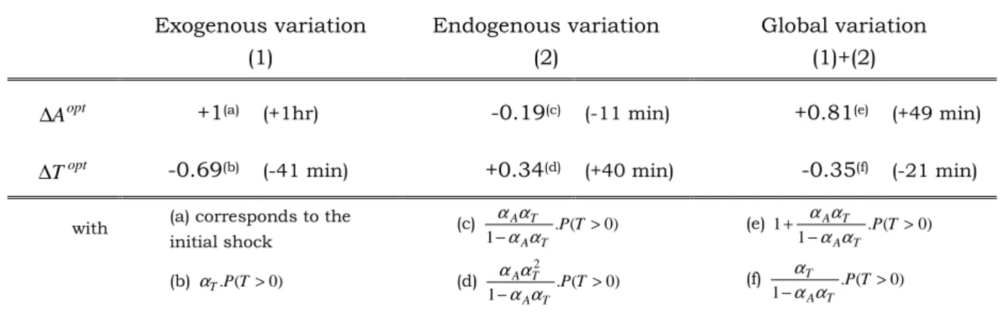
To investigate the intensity of these relations, we estimated the two reciprocal marginal effects. We first estimated the effect of a shock providing to each individual incentive to devote to parental care one more hour a week. Table 4 reports the optimal time allocation variation and a decomposition of this variation into an exogenous variation and an endogenous variation. The former supposes that the caregiving behaviour is exogenous in the sense that it does not depend on hours worked12. In the latter, the additional effect induced by the endogeneity of the caregiving behaviour is tacking into account. On average, the initial shock on time devoted to care produces a final decrease of working time by 21 minutes, whereas the optimal caregiving time, after adjustment, finally increases by 49 minutes. The working time reduction is thus relatively high. Two reasons may explain this effect. First, the analysis is focused on the women aged 50 to 65 that is a population for whom the caregiving behaviour may interact with the retirement decision. Some women may then leave the labour market in order to provide care for their disabled parent, in particular when others sources of care are not available. Following the decomposition proposed by
McDonald and Moffit (1980), we show that 51 % of this the working time decrease (that is 11 minutes) comes from the decrease of the probability to work13. Second, individual labour behaviour also depends on the labour demand, which is not taken into account in our model. In particular, if individuals may only choose between two work contracts (full time or part-time work), they may be constrained to reduce their working time more than they would in order to provide care for their parent.
Similarly, Table 5 reports the optimal time allocation variation after a positive exogenous shock on the working time. After adjustment, the caregiving time variation appears relatively small (+5 minutes).
Table 4: Average effect on an exogenous caregiving time variation on the optimal time allocation Exogenous variation (1) Endogenous variation (2) Global variation (1)+(2) opt A
∆ +1(a) (+1hr) -0.19(c) (-11 min) +0.81(e) (+49 min)
opt T
∆ -0.69(b) (-41 min) +0.34(d) (+40 min) -0.35(f) (-21 min)
with (a) corresponds to the initial shock (c) . ( 0) 1− A T PT> T A α α α α (e) . ( 0) 1 1 > − + PT T A T A α α α α (b) αT.P(T>0) (d) . ( 0) 1 2 > − A T PT T A α αα α (f) . ( 0) 1− A T PT> T α α α
12 This effect may be seen as the working time variation in a situation where the individual is virtually constraint to provide one more hour of care a week. Note that in this situation the time allocation is not optimal for the individual.
13 The remaining 49% corresponds to the effect on the time spent working conditionally on working. This decomposition is however constraint here by the fact that our model does not separately estimate the effect of caregiving on the probability to work and on the number of hours worked conditionally on working. From this point of view, a selection model estimated in two steps could be more appropriate.
Table 5: Average effect on an exogenous working time variation on the optimal time allocation Exogenous variation (1) Endogenous variation (2) Global variation (1)+(2) opt T
∆ +1(a) (+1hr) -0.16(c) (-10 min) +0.84(e) (+50 min)
opt A
∆ +0.18(b) (+11 min) -0.09(d) (-5 min) +0.09(f) (+5 min)
with (a) corresponds to the initial shock (c) . ( 0) 1− A T P A> A T α αα α (e) . ( 0) 1 1 > − + PA T A A T α αα α (b) αA.P(A>0) (d) . ( 0) 1 2 > − A T P A A T α αα α (f) . ( 0) 1− A T P A> A α α α
To extend the comparison of our empirical results with those expected from our microeconomic model, we simulate specific shocks on the non labour income, on the parent’s health status and on the number of siblings. Consistently with our expectations, findings indicate first that a 1000 Euros increase of the monthly non labour income leads on average to a decrease in time spend working by 6 hours and 43 minutes a week and an increase in caregiving time by 30 minutes a week. Second, when the parent’s health status go from “fear” to “poor”, time devoted to care rises on average by 58 minutes a week whereas working time decreases by 29 minutes a week. Finally, having one more brother reduces caregiving time by 12 minutes a week and increases working time by 6 minutes a week whereas having one more sister reduces caregiving time by 24 minutes a week and increases working time by 12 minutes a week.
7. Robustness analysis
To check the robustness of our results, we first partially relax the coherency condition. Situations with multiple equilibria may arise when the two parameters αA and αT are both negative and when the product αA.αT is higher than 1. Three potential equilibrium may
then exist (one interior equilibrium and two corner equilibria, see figure 3). In this case, we add to the model A (14) a selection rule which allows to select a particular equilibrium among the three potential equilibria14 (Krauth, 2006). However, we still impose the coherency condition when the parameters αA and αT are both positive because in this case,
individuals choose to increase their working and caregiving time until that time devoted to leisure be equal to zero, which seems unrealistic. Results obtained are strictly unchanged in comparison with those report in table 3 since the likelihood function still converges to the same value (each daughter been characterized by a single equilibrium).
14 Four different exogenous selection rules have been tested. The first assumes that each equilibrium has an equal probability (1/3) to be optimal and then chosen by the daughter. The three others assume than one of the three equilibria is always optimal and then always chosen by the daughter. The different likelihoods of each specification are available upon request. See Bjorn and Vuong (1985), Fontaine et al. (2009), Krauth (2006), Soetevent & Kooreman (2007) or Tamer (2003) for similar approaches in a simultaneous discrete model.
We have also compared our results with those obtained by a pseudo IV approach. We first estimated the following model:
> = otherwise if 0 0 * * i i opt i T T T and > = otherwise if 0 0 * * i i opt i A A A with + + + = + + + = ' ' ' * ' ' ' ' * Ai T A Ai A i A i Ti opt i T Ti T i T i u x x x A u A x x T λ β δ α β δ (25)
The specification of the working time equation is unchanged compared to model A (14). However, contrary to previous model, the second equation is used to instrument the caregiving time. This approach is similar to the one used by Crespo (2007) and Johnson & La Sasso (2000), which only focus on the causal effect of the caregiving time on the working time, that is on the parameter αT' . Every variable which could directly or indirectly (through
the working time) influence the care provision are included as explanatory variables in the caregiving time equation (the vector xAi then gathers the excluded instruments). The two
equations are jointly estimated by maximum likelihood method, allowing the residuals of the two equations to be correlated. Estimation results are very close from those obtained with the model A. In particular, the estimated effect of an exogenous variation of caregiving time is still significant (at the 1% level) and negative. The marginal effect is however slightly higher (in absolute value): on average, one more hour of caregiving decreases by 25 minutes working time.
The same approach is used to estimate the reverse causality. The model estimated is then the following: > = otherwise if 0 0 * * i i opt i T T T and > = otherwise if 0 0 * * i i opt i A A A with + + + = + + + = '' '' '' '' * '' '' '' * Ai opt i A Ai A i A i Ti A T Ti T i T i u T x x A u x x x T α β δ λ β δ (26)
Estimation results are also very close from those obtained with the model A: on average one hour more of working time increases time devoted to care by 4 minutes.
7. Conclusion
This paper examines the trade-off between paid work and parental care among European women aged 50 to 65, that is women having a key role in informal care for disabled elderly but who are also encourage to leave the labour market as late as possible.
We first propose a simple time allocation model between labour, care and leisure. From the two first-order conditions defining the optimal time allocation, we jointly estimate the working and caregiving time taking into account the simultaneity of the two decisions and the censure which characterizes each variable. Using data from the second wave of SHARE, our main result suggests that the statistical negative correlation between work and care stem from the significant negative effect of caregiving time on working time. This result may reveal that women aged 50 to 65 give priority to their caregiving responsibility at the expense of paid work, given that they reduce their working time to provide informal care but that they do not reduce their caregiving time when hours worked increase. From a public policy perspective, encouraging the informal care provision for disabled elderly people may then hamper the growth in senior employment.
Our study presents however some limits. First, some potentially important variables are missing in the data set, such as the use of formal care or the parent’s place of residence. In particular, some individuals in the data set may have a parent living in nursing home. Moreover, we excluded from the analysis daughters living with their elderly parent because of a lack on information concerning their caregiving behaviour. Further research could consist in estimating the labour and care behaviour simultaneously with the intergenerational household formation. The paper is focused on the effect of caregiving provision on hours worked. Further research should also consider other potential effects of care on labour behaviour, such as the necessity to obtain more flexible working hours, the reduction in careers prospect or the necessity to take some time off.
Annexe 1: Estimation results without exclusion restrictions (1) * T (2) * A Constant 30.99*** (7.28) -8.92** (4.77)
Country dummies Yes Yes
Daughter characteristics
Age 50-51 Ref. Ref.
52-53 -1.94 (3.11) -0.11 (2.12) 54-55 -12.23*** (3.35) 2.82 (2.22) 56-57 -20.31*** (3.84) 3.79 (2.38) 58-59 -22.94*** (4.44) 1.91 (2.72) 60-61 -47.59*** (7.35) 3.31 (3.20) 62-63 -51.24*** (8.95) 2.24 (3.74) 64-65 -55.35*** (13.31) 4.91 (4.12)
Education level Pre-primary or primary education Ref. Ref.
Lower secondary education -2.06 (3.89) 1.75 (2.18)
Upper secondary education 7.28** (3.58) 0.06 (2.03)
Post secondary education 18.58*** (3.81) 1.40 (2.27)
Health status « poor » -22.18*** (5.71) -1.28 (2.93)
« fair » -10.91*** (2.91) -0.71 (1.70)
« good » Ref. Ref.
« very good » 1.11 (2.99) 2.40 (1.80)
« excellent -1.40 (3.79) -0.10 (2.29)
Martial status Not married Ref. Ref.
Married -10.29*** (2.59) 1.26 (1.57)
Number of children 0 Ref. Ref.
1 1.11 (5.08) 0.74 (3.04)
2 or more -1.40 (2.87) -0.63 (1.73)
Log of the monthly non labour income -4.65*** (0.36) 1.30*** (0.26)
Siblings characteristics
Number of brothers 0 Ref. Ref.
1 2.02 (2.65) -1.30 (1.54)
2 or more 1.91 (2.92) -2.01 (1.75)
Number of sisters 0 Ref. Ref.
1 -1.66 (2.73) -3.35** (1.58)
2 or more 0.29 (2.82) --3.93** (1.66)
Eldest child no Ref. Ref.
yes 4.05 (2.61) 1.96 (1.54)
Youngest child no Ref. Ref.
yes 3.47 (3.02) 0.72 (1.81)
Parent characteristics
Gender Woman Ref. Ref.
Man 1.71 (3.16) -4.98*** (2.01) Age ]- ; 74] -1.20 (6.31) -16.27*** (5.67) [75 ; 79] 0.04 (3.27) -2.81 (2.12) [80 ; 84] Ref. Ref. [85 ; 89] 4.40 (2.74) 1.02 (1.65) [90 ; 94] 2.13 (3.97) 2.89 (2.22) [95 ; +] 10.62 (6.54) 6.65** (3.34)
Health status "fair" Ref. Ref.
(continued…) Not constraint Model (1) * T (2) * A
Geographical proximity Less than 1 km away Ref. Ref.
Between 1 and 5 km away -4.72 (3.96) -7.83*** (2.02)
Between 5 and 25 km away -3.53 (3.70) -10.17*** (1.94)
Between 25 and 100 km away -2.81 (4.14) -14.95*** (2.29)
Between 100 and 500 km away -3.19 (4.49) -19.09*** (2.67)
More than 500 km away -7.32 (5.17) -22.63*** (3.49)
Interactions betwen work and care
Hours of caregiving ( A ) -1.91*** (0.28) .
Hours of work ( T ) . 0.55*** (0.09)