Kinematic and Dynamic Analyses of the Orthoglide 5-axis

HAL Id: hal-00322702

https://hal.archives-ouvertes.fr/hal-00322702

Submitted on 18 Sep 2008

HAL is a multi-disciplinary open access archive for the deposit and dissemination of sci-entific research documents, whether they are pub-lished or not. The documents may come from teaching and research institutions in France or abroad, or from public or private research centers.

L’archive ouverte pluridisciplinaire HAL, est destinée au dépôt et à la diffusion de documents scientifiques de niveau recherche, publiés ou non, émanant des établissements d’enseignement et de recherche français ou étrangers, des laboratoires publics ou privés.

5-axis

Raza Ur-Rehman, Stéphane Caro, Damien Chablat, Philippe Wenger

To cite this version:

Raza Ur-Rehman, Stéphane Caro, Damien Chablat, Philippe Wenger. Kinematic and Dynamic Anal-yses of the Orthoglide 5-axis. Congress on Mechatronics, May 2008, Le Grand-Bornand, France. pp.1-6. �hal-00322702�

Abstract—This paper deals with the kinematic and dynamic

analyses of the Orthoglide 5-axis, a five-degree-of-freedom manipulator. It is derived from two manipulators: i) the Orthoglide 3-axis; a three dof translational manipulator and ii) the Agile eye; a parallel spherical wrist. First, the kinematic and dynamic models of the Orthoglide 5-axis are developed. The geometric and inertial parameters of the manipulator are determined by means of a CAD software. Then, the required motors performances are evaluated for some test trajectories. Finally, the motors are selected in the catalogue from the previous results.

I. INTRODUCTION

ARALLEL kinematics machines become more and

more popular in industrial applications [1, 2].This

growing attention is inspired by their essential advantages over serial manipulators that have already reached the dynamic performance limits. In contrast, parallel manipulators are claimed to offer better accuracy, lower mass/inertia properties, and higher structural stiffness (i.e. stiffness-to-mass ratio) [3]. These features are induced by their specific kinematic structure, which resists to the error accumulation in kinematic chains and allows convenient actuators location close the manipulator base. Besides, the links work in parallel against the external force/torque, eliminating the cantilever-type loading and increasing the manipulator stiffness [4]. The latter makes them attractive for innovative machine-tool architectures [5, 6], but practical utilization for the potential benefits requires development of efficient kinematic and dynamic analyses, which satisfy the computational speed and accuracy requirements of relevant design procedures.

This paper focuses on the kinematic and dynamic analyses of the Orthoglide 5-axis, a spatial parallel-kinematics machine (PKM) developed for high speed operations [7]. To evaluate the forces and torques that have to be exerted by the actuators of the Orthoglide 5-axis, its kinematic and dynamic analyses are of primary importance.

II. ORTHOGLIDE 5-AXIS

The Orthoglide 5-axis, illustrated in Fig. 1, is derived from a 3-dof translating manipulator, the Orthoglide 3-axis and a 2-dof spherical wrist [7].

Fig. 1. The Orthoglide 5-axis

The Orthoglide 3-axis is a Delta-type PKM [8] dedicated to 3-axis rapid machining applications developed at the Research Institute in Communications and Cybernetics of Nantes (IRCCyN) [9]. This mechanism is composed of three identical legs. Each leg is made up of a prismatic joint, a revolute joint, a parallelogram joint and another revolute joint. The first joint, i.e. the prismatic joint of each leg, is actuated while the end-effector is attached to the other end of each leg. Hence, the Orthoglide 3-axis is a PKM with movable foot points and constant chain lengths.

Fig. 2. The Orthoglide 3-axis

The Orthoglide 3-axis gathers the advantages of both serial and parallel kinematic architectures such as regular workspace, homogeneous performances, good dynamic performances and stiffness. The interesting features of the Orthoglide 3-axis are large regular dextrous workspace, uniform kinetostatic performances, good compactness [10] and high stiffness [11].

The two-dof spherical wrist that is implemented in the

Kinematic and Dynamic Analyses of the Orthoglide 5-axis

R. Ur-Rehman, S. Caro, D. Chablat, P. Wenger

Institut de Recherche en Communication et Cybernétique de Nantes, UMR CNRS 6597, 1 rue de la Noë, 44321 Nantes, France

Raza.Ur-Rehman@irccyn.ec-nantes.fr

Orthoglide 5-axis is derived from the Agile Eye, a three-dof spherical wrist developed by Gosselin and Hamel [12]. Nevertheless, the two-dof spherical wrist was designed in order to have high stiffness, [13]. A CAD model of the wrist is shown in Fig. 3. It consists of a closed kinematic chain composed of five components: the proximal 1, the proximal 2, the distal, the terminal and the base. These five links are connected by means of revolute joints, the two revolute joints connected to the base being actuated. Let us notice that the revolute joints axes intersect.

Fig. 3. Spherical wrist of the Orthoglide 5-axis III. TRAJECTORY PLANNING

In order to analyze the kinematic and dynamic performance of the Orthoglide 5-axis, two test trajectories are proposed. The inverse kinematic and dynamic problems of the manipulator are solved for both trajectories.

The Orthoglide 5-axis is designed for a

500x500x500 mm3 _{cubic workspace. Let us notice that the}

cubic workspace center, i.e., point I , and the origin O of the reference frame, and the intersection of the prismatic joints axes, do not coincide as explained in[9] and shown in Fig. 4. The vectorOIuur, expressed by dr = [dx dy dz]T_{, is also called}

position vector of the cubic workspace center. Here, the geometric centre of the path of the test trajectories is supposed to be point I. Accordingly, the test trajectories are defined as follows:

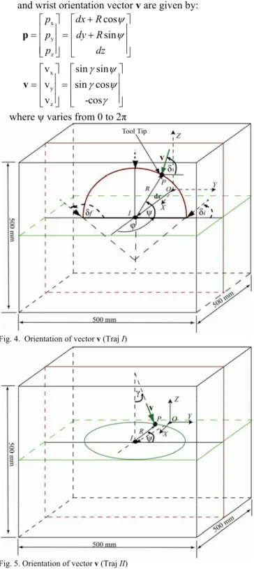
• Traj. I: semi-circular trajectory in a plane perpendicular to XY-plane defined by radius R , trajectory angle ψ with Y-axis, trajectory plane orientation angle φ (angle between the trajectory plane and X-axis) and vector v orientation angle δ (Fig. 4). Position vector p and wrist orientation vector v are given by:

x y z cos cos cos sin cos p dx R p dy R p dz R ψ ϕ ψ ϕ ψ + ⎡ ⎤ ⎡ ⎤ ⎢ ⎥ ⎢ ⎥ =_{⎢ ⎥ ⎢}= + _⎥ ⎢ ⎥ ⎢ + ⎥ ⎣ ⎦ ⎣ ⎦ p x y z v cos cos v cos sin v sin δ ϕ δ ϕ δ − ⎡ ⎤ ⎡ ⎤ ⎢ ⎥ ⎢ ⎥ =_{⎢ ⎥ ⎢}= − _⎥ ⎢ ⎥ ⎢ − ⎥ ⎣ ⎦ ⎣ ⎦ v

where δ varies from π/6 to 5π/6 and ψ varies from 0 to π..

• Traj. II: circular trajectory in horizontal or XY-plane defined by radius R, vector v, constant orientation angle γ with Z-axis and the angle ψ (Fig. 5). Position vector p and wrist orientation vector v are given by:

x y z cos sin p dx R p dy R p dz ψ ψ + ⎡ ⎤ ⎡ ⎤ ⎢ ⎥ ⎢ ⎥ =_{⎢ ⎥ ⎢}= + _⎥ ⎢ ⎥ ⎢ ⎥ ⎣ ⎦ ⎣ ⎦ p x y z v sin sin v sin cos v -cos γ ψ γ ψ γ ⎡ ⎤ ⎡ ⎤ ⎢ ⎥ ⎢ ⎥ =_{⎢ ⎥ ⎢}= _⎥ ⎢ ⎥ ⎢ ⎥ ⎣ ⎦ ⎣ ⎦ v

where ψ varies from 0 to 2π

Fig. 4. Orientation of vector v (Traj I)

Fig. 5. Orientation of vector v (Traj II)

Let us notice that several test trajectories can be derived from Traj. I and Traj. II, by changing their parameters.

IV. KINEMATIC ANALYSIS

A. Orthoglide 3 axis

The geometric parameters of the Orthoglide 3-axis are defined as a function of the size of a prescribed cubic Cartesian workspace, that is free of singularities and internal collision

The kinematic architecture of the Orthoglide-3axis is shown in Fig. 2 where A1B1, A2B2 and A3B3 represent the prismatic joints and P is the end-effector. Due to its Delta-linear architecture, the Orthoglide-3axis is a translating parallel manipulator with 3-DOF.

A simplified model of the Orthoglide 3-axis is illustrated in Fig. 6 [14] in which three links of length L are connected by means of a spherical joint to end-effector “P” at one end and to the corresponding prismatic joints “Ai” at the other

end. θx, θy and θz are the angles between the links and the

corresponding prismatic joints axes. The reference frame is coincident with the prismatic joint axes; it is the origin being the intersection point of those axes. The input position vector of the prismatic joint variables is represented by

(

)

ρ and the output position vector of the

end-effector by p=

(

)

Fig. 6. Simplified model of the Orthoglide 3-axis

Using these notations, the inverse kinematic relations for a spherical singularity free workspace can be written as [10]

2 2 2 2 2 2 2 2 2 x x y z y y x z z z x y p L p p p L p p p L p p ρ ρ ρ = + − − = + − − = + − −

Due to the Orthoglide geometry and manufacturing technology, the displacement of its prismatic joints is bounded [10], namely,

, ,

0≤ρ_{x y z} ≤2L

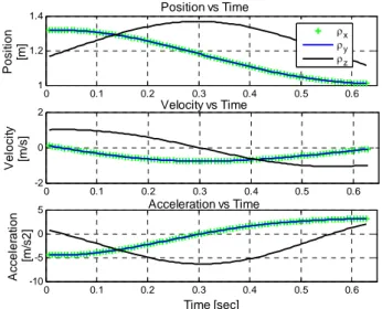
The kinematic performance of the Orthoglide 3-axis is analyzed by means of the foregoing test trajectories. The velocity of end-effector P throughout the trajectory, is

supposed to be constant i.e. Vp= 1 m/s. Accordingly the

actuated prismatic joints position, rates and acceleration are

plotted in Figs. 7 to 9 for both test trajectories, the radius of their path being equal to 0.2 m.

0 0.1 0.2 0.3 0.4 0.5 0.6 0.5 1 1.5 Po s it io n [m] Position vs Time 0 0.1 0.2 0.3 0.4 0.5 0.6 -2 -1 0 1 2 Ve lo c it y [m/s ] Velocity vs Time 0 0.1 0.2 0.3 0.4 0.5 0.6 -10 -5 0 5 10 Time [s] A ccel e ra ti o n [m/s 2 ] Acceleration vs Time ρx ρ_y ρ_z

Fig. 7. Actuated prismatic joints position, rates and acceleration of the Orthoglide 3-axis for Traj I with φ=90˚

0 0.1 0.2 0.3 0.4 0.5 0.6 1 1.2 1.4 Po s it io n [m ] Position vs Time 0 0.1 0.2 0.3 0.4 0.5 0.6 -2 0 2 Ve lo c it y [m /s ] Velocity vs Time 0 0.1 0.2 0.3 0.4 0.5 0.6 -10 -5 0 5 Time [sec] A cce le ra ti o n [m /s 2 ] Acceleration vs Time ρ_x ρy ρ_z

Fig. 8. Actuated prismatic joints position, rates and acceleration of the Orthoglide 3-axis for Traj I with φ=45˚

0 0.2 0.4 0.6 0.8 1 1.2 0.5 1 1.5 Po s it io n [m ] Position vs Time 0 0.2 0.4 0.6 0.8 1 1.2 -2 0 2 V e loci ty [m/ s ] Velocity vs Time 0 0.2 0.4 0.6 0.8 1 1.2 -10 0 10 Time [s] A c cel e rat io n [m /s 2 ] Acceleration vs Time ρ_x ρ_y ρ_z

Fig. 9. Actuated prismatic joints position, rates and acceleration of the Orthoglide 3-axis for Traj II with γ=45˚

Fig. 7 shows the kinematic performance required by the prismatic actuators when end-effector P moves in YZ-plane. Even if P does not move along X-axis, the displacement of the prismatic actuator mounted along X-axis is not null. Fig. 8 and Fig. 9 display the required kinematic performance of the motors when P follows Traj I (φ=45˚) and Traj II

(γ=45˚), respectively for R=0.2m. The maximum velocities

and accelerations of the prismatic actuators required for the three test trajectories are shown in Table I. We can notice that the maximum prismatic joint velocity is equal to 1 m/s whereas its maximum acceleration is equal to 6.31 m/s2_.

TABLE I.

MAXIMUM PRISMATIC JOINTS RATES AND ACCELERATIONS

Test Trajectory Max Absolute Velocity [m/s] Max Absolute Acceleration [m/s2_] Vx Vy Vz Ax Ay Az Traj I, γ=90˚ 0.12 1.01 1.06 0.62 6.32 6.32 Traj I, γ=45˚ 0.77 0.77 1.07 4.51 4.51 6.33 Traj II, γ=45˚ 1.06 1.06 0.12 6.31 6.31 0.66 B. Spherical Wrist

The spherical wrist mechanism of the Orthoglide 5-axis consists of a closed kinematic chain composed of five components: proximal-1, proximal-2, distal, terminal and the base. These five links are connected by means of revolute joints, of which axes intersect. Besides, only the two revolute joints connected to the base of the wrist are actuated. The distal has an imaginary axis of rotation passing through the intersection point of other joint axis and perpendicular to the plane of proximal-2.

The kinematic equations of the wrist are written by means of six reference frames attached to the six rigid bodies and the corresponding Denavit-Hartenberg (DH)-parameters. Fig. 10 shows the orientation of these reference frames while vector v represents the orientation of the terminal of the wrist, i.e. the cutting tool. Moreover, α0 denotes the

angle between e1 and e2 while αi denotes the angle between

ei and ei+2 (i = 1…4).

Fig. 10. Orientations of reference frames for the Orthoglide Wrist

The reference frame R1 is defined in such a way that the

Z1-axis coincides with e1 and e2 lies in the X1Z1-plane.

Similarly R2 has its Z2-axis in the direction of e2 and e1 lies

in the X2Z2-plane. Reference frame Ri(i = 3, 4, 5, 6) with

Zi = ei are defined by the rotation of frame Ri-2 and

following the DH conventions.

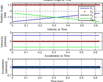
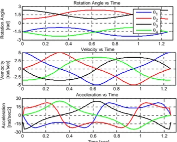
Finally, the inverse kinematic problem of the wrist can be derived from the definitions of the reference frames and unit vectors to develop the relations between the joints angles (θ1, θ2, θ3, θ4) [15]. Fig. 11 to Fig. 13 display the revolute

joints angles, rates and accelerations for the two trajectories introduced in Section III, the radius of their path being equal to 0.2 m. 0 0.1 0.2 0.3 0.4 0.5 0.6 -0.1 0 0.1 Acceleration vs Time Time [sec] A cce le ra ti o n [r a d /se c2 ] 0 0.1 0.2 0.3 0.4 0.5 0.6 -3 -1.5 0 1.5

Rotation Angle vs Time

R o ta ti on A ngl e [r ad] 0 0.1 0.2 0.3 0.4 0.5 0.6 -5 0 5 Velocity vs Time Ve m o c ity [r ad/ s e c ] θ₁ θ₂ θ₃ θ₄ Fig. 11. Revolute joints angles, rates and accelerations of the wrist (Traj I, φ=90˚) 0 0.1 0.2 0.3 0.4 0.5 0.6 -3 -1.5 0 1.5 3

Rotation Angle vs Time

R o ta ti on A ngl e [r a d ] 0 0.1 0.2 0.3 0.4 0.5 0.6 -5 -2.5 0 2.5 5 Velocity vs Time Ve m o c it y [r ad/ s e c ] 0 0.1 0.2 0.3 0.4 0.5 0.6 -10 0 10 Acceleration vs Time Time [sec] Ac c e le ra ti o n [r ad /s ec 2] θ₁ θ₂ θ₃ θ₄

Fig. 12. Revolute joints angles, rates and accelerations of the wrist (Traj I, φ=45˚)

Fig. 11 is the case where wrist end-effector moves in the

YZ-plane (φ=90˚) so only one of the wrist actuator (θ1)

works, while Fig. 12 and Fig. 13 represent the cases where both of the actuators work. Compared to Traj I, both wrist actuators experience greater velocities and accelerations for Traj II (max velocity=5 m/s and max acceleration=22 m/s2_).

This can be explained by the higher order variations of rotation angles in Traj II to that of linear variation of rotation angles in Traj I

0 0.2 0.4 0.6 0.8 1 1.2 -3

-1.5 0 1.5

3 Rotation Angle vs Time

R o ta ti o n A n g le [r a d ] 0 0.2 0.4 0.6 0.8 1 1.2 -5 -2.5 0 2.5 5 Velocity vs Time Ve m o c it y [r ad /s ec ] 0 0.2 0.4 0.6 0.8 1 1.2 -30 -15 0 15 30 Acceleration vs Time Time [sec] Ac c e le ra ti o n [r ad /s ec 2 ] θ1 θ2 θ3 θ4

Fig. 13. Revolute joints angles, rates and accelerations of the wrist (Traj II, γ=45˚)

V. DYNAMIC ANALYSIS

A. Orthoglide 3-axis

The dynamic analysis of the Orthoglide 3-axis is performed in order to evaluate the torques required by the three actuated prismatic joints. Here, we take advantage of the dynamic model developed in [16]. The geometric and dynamic parameters used in the analysis are obtained from SYMORO+ (SYmbolic MOdeling of Robots), a software for the automatic generation of symbolic model of robots [17] and defined in [16]. Fig. 14 illustrates a leg of the Orthoglide with the definition of the parameters and the frames attached to all the bodies [16].

Fig. 14. Orthoglide leg parameterization for the dynamic analysis

The geometric, mass and inertial parameters used in the dynamic model were determined for the Orthoglide 5-axis by means of SolidWorks CAD software, and from the

geometry of the mechanism. The dynamic performance of the Orthoglide 3-axis is then evaluated for different test trajectories. The actuators forces required to follow those trajectories are shown in Fig. 15.

TABLE II.

PARAMETERS OF ORTHOGLIDE 3-AXIS REQUIRED FOR DYNAMIC ANALYSIS

Parameters for leg i Symbol Mass of the platform (wrist) mp

Mass of body 1 m1i

Mass of bodies 2 and 4 m2i, m4i

Mass of bodies 3 and 7 m3i, m7i

Length of parallelograms d4i

Width of parallelograms 2 r2i

Actuators moment of inertia Imi

0 0.1 0.2 0.3 0.4 0.5 0.6 -1000

-500 0

500 Actuators Forces vs Time (Traj-I, φ = 90 deg)

Fo rc e [ N ] 0 0.1 0.2 0.3 0.4 0.5 0.6 -1000 -500 0

Actuators Forces vs Time (Traj-I, φ = 45 deg)

Fo rc e [ N ] 0 0.2 0.4 0.6 0.8 1 1.2 -1000 -500 0

500 Actuators Forces vs Time (Traj-II, γ = 45 deg)

Time [sec] Fo rc e [ N ] Actuator1(ρ_y) Actuator2(ρ_x) Actuator3(ρ_z)

Fig. 15. Orthoglide 3-axis actuators forces (Traj-I and II)

B. Spherical Wrist

A Newton approach is used to come up with the dynamic modeling of the Orthoglide wrist. A similar methodology was also used in [15]. Let us assume that:

• friction forces are neglected;

• there is a spherical joint is between the distal and the terminal link in order to get an isostatic mechanism; • there is a planar joint between the distal and the

proximal-2.

Thus, the free body diagrams of terminal, distal, proximal-1 and proximal-2 can be drawn. The equilibrium equations are written for each free body diagram and then, the equations used to evaluate the actuators torques are obtained [15]. The latter are shown in Fig. 16. It can be seen that for YZ-plane trajectory (Traj I, φ = 90˚), only the first actuator, aligned with the Y-axis (Fig. 4) experiences the torque, while for other two test trajectories both actuators work and experience torques. Second actuator, aligned with

X-axis, experiences greater torque compared to the first

actuator for Traj I, φ = 45˚and for Traj II

In order to verify the results obtained with the Newton approach, the principle of virtual work is used.

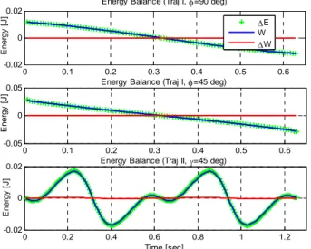
energies i.e. ΔKE and ΔPE are evaluated during a time interval dt. The total energy variation ΔE over dt is defined as ΔE = ΔKE + ΔPE. Therefore, the total virtual work W is calculated by the product of the mean torques and the corresponding angular displacement during each time interval dt. i.e.,

1. 1 1. 2

W= Δ + Δ T θ T θ

1

T and T being the mean torques of actuators 1 and 2, 2

respectively during dt, respectively.

0 0.1 0.2 0.3 0.4 0.5 0.6 -0.8 -0.4 0 0.4 0.8

Actuators Torques vs Time (Traj I, φ=90 deg)

To rq u e [ N m] Actuator 1 Actuator 2 0 0.1 0.2 0.3 0.4 0.5 0.6 -1.2 -0.6 0 0.6

1.2 Actuators Torques vs Time(Traj I, φ=45 deg)

T o rq ue [ N m ] 0 0.2 0.4 0.6 0.8 1 1.2 -2 -1 0 1

2 Actuators Torques vs Time (Traj II, γ=45 deg)

Time [sec] T o rq u e [N m ]

Fig. 16. Spherical wrist actuators torques (Traj-I and II)

It is noteworthy that the difference between the global

virtual work W and ΔE should be null due to energy

conservation. Accordingly, we compute the difference

between W and ΔE and check the dynamic model of the

wrist, i.e., ΔW= ΔE-W. This difference is highlighted in Fig. 17 for the three test trajectories that are considered in the scope of the study. It turns out ΔW is null in all cases. Consequently, the dynamic model of the wrist makes sense.

0 0.1 0.2 0.3 0.4 0.5 0.6 -0.02

0 0.02

Energy Balance (Traj I, φ=90 deg)

0 0.1 0.2 0.3 0.4 0.5 0.6 -0.05

0

0.05 Energy Balance (Traj I, φ=45 deg)

0 0.2 0.4 0.6 0.8 1 1.2 -0.02

0

0.02 Energy Balance (Traj II, γ=45 deg)

Time [sec] E ner gy [ J ] E ner gy [ J ] E ner gy [ J ] ΔE W ΔW

Fig. 17. Energy balance for wrist dynamics (Traj-I and II)

VI. CONCLUSION

This paper dealt with the kinematic and dynamic analyses of the Orthoglide 5-axis, a five-degree-of-freedom

manipulator. First, it turned out that kinematic and dynamic analyses of the translating part and the spherical wrist of the manipulators can be decoupled. The geometric and inertial parameters of the manipulator were determined by means of a CAD software. We came up with the dynamic model of the spherical wrist by means of a Newton approach. Besides, this model has been checked with the principle of virtual work. Then, the required motors performances were evaluated for some test trajectories. Various simulations results showed that the FFA 20-80 harmonic drive motors of 0.8 kW and the NX430 EAF motors of 1.8 kW, primarily selected for the wrist and Orthoglide 3-axis respectively, are suitable for the prototype of the Orthoglide 5-axis. In future works, friction forces as well as payload will be considered in the dynamic analysis and further test trajectories will be performed.

REFERENCES

[1] T.Brogardh, “Present and future robot control development - An industrial perspective,” Annual Reviews in Control, 31(1), pp. 69-79, 2007

[2] H. Chanal, E. Duc, and P. Ray, “A study of the impact of machine tool structure on machining processes”. International Journal of Machine Tools and Manufacture, 46(2), pp. 98-106, 2006.

[3] J.-P. Merlet, Parallel Robots, 2nd Edition. Springer, Heidelberg, 2005. [4] L. W. Tsai, Robot analysis: The Mechanics of Serial and Parallel

Manipulators, John Wiley & Sons, New York, 1999.

[5] J. Tlusty, J. C. Ziegert, and S. Ridgeway, “Fundamental comparison of the use of serial and parallel kinematics for machine tools,” CIRP Annals, 48(1), pp. 351–356, 1999

[6] O. Company, and F. Pierrot, “Modelling and Design Issues of a 3-axis Parallel Machine-Tool,” Mechanism and Machine Theory, 37(11), pp 1325-1345, 2002

[7] D. Chablat et P. Wenger, “Device for the movement and orientation of an object in space and use thereof in rapid machining”, Centre National de la Recherche Scientifique /Ecole Centrale de Nantes, European patent: EP1597017, US patent: 20070062321, 2005.

[8] R. Clavel, "Delta, a fast robot with parallel geometry", Proc. 18th

International Symposium on Industrial Robots, 1988, pp.91-100. [9] D. Chablat, and P. Wenger, “Architecture Optimization, of a 3-DOF

Parallel Mechanism for Machining Applications, The Orthoglide,” IEEE Trans. on Robotics and Automation 19, 2003, pp.403–410. [10] A. Pashkevich, P. Wenger and D.Chablat, “Design Strategies for the

Geometric Synthesis of Orthoglide-type Mechanisms”, Journal of Mechanism and Machine Theory, Vol. 40(8), 2005, pp. 907-930. [11] A. Pashkevich, D. Chablat and P. Wenger, “Stiffness Analysis of

3-d.o.f. Overconstrained Translational Parallel Manipulators”, Proc. IEEE Int. Conf. Rob. and Automation, May 2008.

[12] C. Gosselin, and J.F. Hamel, “The agile eye: a high performance three-degree-of-freedom camera-orienting device,” IEEE Int. conference on Robotics and Automation, San Diego, 1994, pp. 781-787.

[13] D. Chablat, and P. Wenger, “A six degree of freedom Haptic device based on the Orthoglide and a hybrid Agile Eye,” 30th Mechanisms & Robotics Conference (MR), Philadelphia, USA, 2006.

[14] A. Pashkevich, D. Chablat and P. Wenger, “Kinematics and Workspace Analysis of a Three-Axis Parallel Manipulator: the Orthoglide,” Robotica, Vol 24 , Issue 1, 2006, Pages: 39 - 49

[15] F. Caron, “Analyse et conception d'un manipulateur parallèle sphérique à deux degrés de liberté pour l'orientation d'une caméra,” M.S. thesis, Laval University, Quebec, QC, Canada, 1997.

[[16] S. Guégan, "Contribution à la modélisation et l'identification dynamique des robots parallèles." Ph.D. Thesis, Ecole Centrale de Nantes, Nantes, France, 2003

[[17] W. Khalil and D. Creusot , "SYMORO+: a system for the symbolic modelling of robots", Robotica, Vol. 15, pp. 153-161, 1997