Dependability of Fault-Tolerant Systems — Explicit Modeling of the Interactions Between Hardware and Software Components

(1)

HAL Id: hal-01976182

https://hal.laas.fr/hal-01976182

Submitted on 9 Jan 2019

HAL is a multi-disciplinary open access

archive for the deposit and dissemination of sci-entific research documents, whether they are pub-lished or not. The documents may come from teaching and research institutions in France or abroad, or from public or private research centers.

L’archive ouverte pluridisciplinaire HAL, est destinée au dépôt et à la diffusion de documents scientifiques de niveau recherche, publiés ou non, émanant des établissements d’enseignement et de recherche français ou étrangers, des laboratoires publics ou privés.

Dependability of Fault-Tolerant Systems - Explicit

Modeling of the Interactions Between Hardware and

Software Components

Karama Kanoun, Marie Borrel

To cite this version:

Karama Kanoun, Marie Borrel. Dependability of Fault-Tolerant Systems - Explicit Modeling of the Interactions Between Hardware and Software Components. 2nd Annual IEEE International Computer Performance and Dependability Symposium (IPDS’96), 4-6 septembre 1996, pp.252-261, Sep 1996, Urbana-Champaign, United States. �hal-01976182�

(2)

2nd Annual IEEE International Computer Performance and Dependability Symposium (IPDS'96), Urbana-Champaign (USA), 4-6 septembre 1996, pp.252-261

Abstract

This paper addresses the dependability modeling of hardware and software fault-tolerant systems taking into account explicitly the interactions between the various components. It presents a framework for modeling these interactions based on Generalized Stochastic Petri Nets (GSPNs). The modeling approach is modular: the behavior of each component and each interaction is represented by its own GSPN, while the system model is obtained by composition of these GSPNs. The composition rules are defined and formalized through clear identification of the interfaces between the component and the dependency nets. In addition to modularity, the formalism brings flexibility and re-usability. This approach is applied to a simple, but still representative, example.

1. Introduction

In the context of computer system dependability, the need for addressing simultaneously both hardware and software dependability aspects has now been recognized. However, even though a number of publications have been devoted to the dependability of combined hardware and software systems (see e.g. [5, 6, 13, 14]), work on both aspects dealt with at the same time is not prevalent. Also, it is noteworthy that, when they are considered together for real-life systems, the interactions between the components are not usually modeled explicitly (see e.g. [15, 16, 20]).

This paper addresses the dependability modeling of hardware and software fault-tolerant systems taking into account the interactions between the various components. These interactions result for example from components communications for functional purposes (i.e., functional interactions), or from the structure of the system, mainly the distribution of software components onto the hardware components (i.e., structural interactions), or from fault tolerance and maintenance strategies (reconfiguration and maintenance interactions). They

induce dependencies between at least two components that are usually stochastic in nature. As a result, system dependability cannot simply be obtained by combining the dependability of its components. An overall model accounting for these dependencies is thus needed. Our aim is to model explicitly these dependencies so as to quantify their influence on system dependability. This is of prime importance during the design of a new system or while upgrading an already existing one. The designer can make different assumptions about the interactions between the components and compare the dependability of the resulting alternative solutions through sensitivity studies. As the nature of interactions is strongly linked to the modeling level considered and the assumptions made at the considered level, it is not possible to model all the interactions that could take place for any fault-tolerant system. Rather, we define a framework for modeling these interactions in a systematic way and, more generally, we define a framework to build up the depend-ability model of a fault-tolerant system explicitly taking into account these interactions. To do this, we follow a modular approach based on Generalized Stochastic Petri Nets (GSPNs) due to their ability to handle modularity and hierarchy. Note that modular approaches using GSPNs or their offsprings are widely used (see e.g., [2, 18] ). Our contribution lies in modeling the interactions between hardware and software components and giving a formal description of these dependencies.

The paper is organized in five sections: Section 2 presents the framework for modeling interactions between hardware and software components. Section 3 gives a formal description of the various types of dependency nets while Section 4 illustrates the approach on a duplex system with several interactions. Section 5 concludes.

2. Modeling Framework

The modeling approach consists in identifying, based on the analysis of the system's behavior, dependencies between the components that could be induced by

func-Dependability of Fault-Tolerant Systems — Explicit Modeling

of the Interactions Between Hardware and Software Components

Karama Kanoun and Marie Borrel

LAAS-CNRS

7, Avenue du Colonel Roche

31077 Toulouse Cedex - France

(3)

tional or structural interactions or by interactions due to system reconfiguration and maintenance. Some examples of dependencies due to these interactions are given in the following. Error propagation between two software com-ponents is an example of stochastic dependency resulting from functional interactions (exchange of data or transfer of intermediate results from one component to another). The halting of the software activities following a perma-nent failure of the hosting hardware is an example of stochastic dependency induced by a structural interaction. Sharing of a single repairman by the two hardware com-puters leads to a maintenance dependency whereas switching from an active component (hardware or software) to a spare component following a permanent failure of the active component leads to a reconfiguration dependency. In this paper, we consider interactions that are driven by events occurring in a component whose occurrence may impact the behavior of other components. A high level model of the system is first derived based on the previous analysis. It is made of blocks and arrows: a block stands for the component model (component net) or a dependency model (dependency net), and an arrow shows the direction of the dependency. The system model is thus obtained by composition of the component and dependency models. In a second step, each block is replaced with its detailed GSPN. To allow for a systematic build up of dependency nets, rules that will have to be followed during model construction are defined. These rules manage the interfaces between the dependency and component nets and are prerequisite for modularity, hierarchical modeling and re-usability (re-usability is a valuable concept when it comes to doing sensitivity studies about certain assumptions regarding a system's behavior or when several alternative solutions are being considered). Also, these rules allow an easy validation of the global model. In the rest of the section, we give the characteristics of the component and dependency nets and present the various types of dependency nets together with the rules that have to be followed to build up the GSPNs.

Components nets: A component net represents the

behavior of a component as resulting from the activation of faults in this component and the subsequent error processing, restart or repair actions. The assumptions made and the degree of detail considered are usually guided by the interactions with other components one wants to exploit (such as the consequences of non detected errors or activation of temporary faults). A component net is designed to be a standalone net with its initial marking, it is live and bounded. It can be connected with dependency nets only following well

de-fined rules as explained hereafter; connections must not alter the initial structure of the component nets.

Dependency nets: A dependency net is linked to at least

two adjacent nets: an initializing and a target net that could be component or dependency nets. To formally describe dependency nets and to promote re-usability, we define as much common characteristics as possible. As a result, whatever is the kind of interaction modeled, all the dependency nets are initialized and interfaced with the adjacent nets following the same rules; they only differ in their effects on the target net. The common characteristics and the different effects on the target nets are introduced in figure 1 where a hypothetical dependency net with all types of effects is given (the notations are introduced with the formalism). They are summarized hereafter.

Action Entry places

Internal transitions

Immediate or timed transition Initializing net (Ni) Dependency net (Nd) Target net (Ng) Tests tij tck tck tij Activation tsj taj ' t aj pen1 pen2 tin 1 tin 2 Authorization pauj taukj pen3 tin3 prem1_j pret 1_j

Figure 1: Characteristics of dependency nets

Dependency net initialization

• A dependency net is initialized through the marking of one or more entry places by the initializing net(s), following firing of initializing transitions in these initializing net(s) (as interactions are event driven). • The initial marking of the entry places is zero.

• When the initializing net is a component net, the consequences of initializing transition(s) firing on the component behavior are modeled within the component net (marking of one or several internal places) and an additional token is generated and deposited in the entry place of the dependency net to activate the interaction.

• If the initializing net is a dependency net, the token deposited in the entry place could be either the one generated when entering the initializing dependency net (corresponding to a series of successive interactions) or an additional one newly generated (corresponding to the initialization in parallel of two or more interactions).

(4)

Internal transitions: The dependency net has internal

transitions (timed or instantaneous) whose firing may be independent from the marking of the adjacent nets (independent transitions) or conditioned by the marking of places in the adjacent nets. A condition is modeled by an inhibitor arc or an arc from and towards the tested place: the marking of this place is not changed. The interfaces with the adjacent nets (excluding initializing arcs and effects on the target nets) are thus only constituted by tests on the marking of specific places. An internal transition could be absorbing (i.e., the tokens are absorbed).

Effects on target nets: These effects are strongly related

to the type of interaction modeled. Thus, three such effects have been identified:

• If the interaction consists in changing the state of another component (the target net is necessarily a component), the effect at the GSPN level involves removal of a token from a stable place (i.e., a place followed by timed transitions, this condition stems from the fact that only stable places correspond to states of the components) in the target net and return of the token to the same place or to another stable place of the target net (immediately or after firing internal transitions in the dependency net). This is referred to as an action net.

• If the interaction consists in performing or synchroniz-ing reconfiguration or maintenance actions, the effects depend on the nature of the initializing net:

- if the initializing net is a component net, the interaction consists in coordinating the component restart (or repair) action with the restart (or repair) action of the components to which it is linked: it requests permission before undertaking internal actions, these actions are enabled by the dependency net (immediately or after firing of internal transitions). The target net is necessarily the same as the initializing net. At the GSPN level, the effect consists of enabling a transition in the component net through the marking of a place in the dependency net. Since the component net is a standalone net, this means that, in the component net, this transition has also to be enabled by the marking of at least an internal place. This is an authorization net,

- if the initializing net is a dependency net, the interac-tion consists in activating another interacinterac-tion with other linked components; at the GSPN level, this consists of initializing another dependency net by de-positing a token in its entry place following the firing of an initializing transition in the initializing dependency net. As previously stated, depending on whether the token deposited in the target net is an

additional one, both dependency nets run in parallel or in series. This is an activation net.

The previous rules are intended to manage the static links between dependency and adjacent nets. Further rules have to be considered to control the dynamic behavior of the nets (i.e., the tokens generation and their flow). They are given together with the formalism in the next section. Note that model construction is an iterative process with information flow in both directions from/to dependency nets to/from components nets: in the component models, care should be taken to include potential dependencies.

Interaction origin and dependency net type: The

interactions have been attributed to three possible origins: functional, structural and those due to system re-configuration and maintenance. Functional and structural interactions are usually accompanied by a state change, the associated nets are thus action nets. Dependencies due to reconfiguration and maintenance may induce a state change and they could be any kind of dependency net.

3. Nets formalization and validation

The aim of this section is to give a formal description of the various rules introduced in the previous section and to address model validation. We first give the main notations, the other notations being defined in table 1.

General Notations

pen_k∈ Pd Entry place (EP) of Nd.

tin_j ∈T_i Transition of Ni that initializes Nd by marking an EP

Mij _{Initializing marking of a dependency net}

tij∈Td Internal independent transition in Nd

tc_k ∈T_d Internal conditioned transition in Nd Interfaces for an action net

taj, t' aj ∈Td Removing and returning action transitions in Nd

prem_k

j ∈Tg Input place in Ng of the removing action trans.taj pretkj ∈Tg Output place in Ng of the returning action trans.t' aj Interfaces for an authorization net

pauj ∈Pd Authorization place of Nd Interfaces for an activation net

ts_k ∈T_d _{Activation transition of Nd}

Table 1: Notations

Let Ni, Nd and Ng denote respectively an initializing, a dependency, and a target net, and let Nx be any of these nets (x = i, d, g). Nx = P

(

x, Tx, Ix, Ox, prx, pax

)

where:

• P_x is the set of places of Nx,.

• T_x = Ttim_x∪ Timm_x is the set of transitions of Nx: Ttim_x

is the set of timed transitions and Timm_x is the set of immediate transitions.

(5)

• _Ox: Tx× Px → N is the output function ( N is the set of

natural integers).

• pr_x the set of timed transitions rates, pa_x the set of firing probabilities of immediate transitions.

The set of places and transitions are such that:

Pi∩ Pd = ∅, Pi∩ Pg= ∅, Pd∩ Pg= ∅, Ti∩ Td = ∅,

T_i∩ Tg = ∅ andTd∩ Tg= ∅

The interfaces of a dependency net Nd with an initializing net Ni and a target net Ng are the input and output functions, I_id, I_dg, O_id, O_dg, that connect places and transitions of Nd to places and transitions of Ni or

Ng. These functions are defined as follows:

Iid: Pi× Td→ N ∪ −1{ } _Idg: Pd× Tg→ N ∪ −1{ }

Oid: Ti× Pd→ N _Odg: Td× Pg→ N

When it is not necessary to distinguish between initializing and target nets, indices i, d, g are omitted.

Initialization: Initializing transitions, entry places and

the initializing marking of a dependency net Nd are defined as follows: let tinj∈Ti and pk ∈Pd such that

O_id

(

tin_j, p_k

)

)

≥ 0 ⇒ Min

( )

pm ≥ Iid

(

pm,tinj

)

(Min: Nd

= -1

2) ∀ pn ∈ P

(

g∪ Pi

)

such that I p

(

n, tck

)

> 0 or

= 0 or

O tc

(

j, pn

)

= 0 with P = P

(

d∪Pi∪ Pc

)

.

Action nets: An action net ends with a transition which causes a token to be removed from a stable place of the target net and to be returned to the same or another stable place of the same net. Removal and return can be done through two distinct transitions (with internal transitions

1 _{I p, t}_{( )}_{≥ 0 ⇒ Mn}

x( )p ≥ I p, t( ) means that there must be enough

tokens in all the input places of t to enable it.

I p, t_{( )}= −1 ⇒ Mnx( )p = 0means that if there is an inhibitor arc

from p to t, there must be no token in p to enable t.

and places between them) or through the same transition. The number of tokens in the target net remains unchanged. Transitions taj and t' aj are action transitions

if the four following conditions are met:

1) ∀ph∈Pi, I p

(

h, taj

= 0(t' aj: returning transition) 3) O t' a

(

j, p'i

)

i =1 Pg

∑

= I p

= O_d

(

t, p_k

)

, p'_k must verify an

equivalent relation.

p_k is then the input place of the removing action taj,

being denoted prem_{k j} and p'_k ,the output place of the

returning transition t' a_j, is denoted pret_{k j} .

Authorization nets: An authorization net ends with one

or several places enabling firing of transitions in the target net(s), authorization places. In this case, the target net is necessarily the initializing net.

pauj ∈ Pd is an authorization place of Nd if:

∀ t ∈Td such that I pau

(

j, t

)

= 0 then ∃ t_{j k} ∈ T

(

i∪ Tg

)

such

that I pau

(

Let Py be such that Py = Pd for action and activation

nets, P_y= P

{

_d − P_aut

}

for authorization nets. The internal places and transitions of a dependency net must satisfy:

(6)

1) Every place has at least one transition that removes tokens: ∀ p ∈Py ∃ t ∈Td I p,t( )> 0 and O t, p( )= 0

2) If there exists an arc with multiplicity x from a place to a transition, there exist x-1 other arcs with multiplicity 1 to x-1, from the same place to x-1 other transitions with the same input and output as the preceding transition:

∀t ∈Td , and p ∈ Py with I p, t( )> 0 and O t, p( )= 0if

∃ p' ∈Pd such that I p, t( )= x, x ∈N then ∃ x transitions

tj ∈Td such that I p' , t

(

j

)

= j, j = 1, ..., x , I p, t

( )

j > 0 and

O t

( )

j, p = 0.

All these transitions are independent internal transitions.

3) if there exists a test arc with multiplicity x between a place and a transition, there exist x-1 other arcs with multiplicity 1 to x-1, from the same place to x-1 other transitions with the same input and output as the preceding transition.

∀ p ∈Py and ∀ p ∈Py with I p, t( )> 0 and O t, p( ) = 0, if

∃ p' ∈P such that I p' , t₍ ₎= O t, p'( )= x, then ∃ x

transitions tj _{such that} I p' , t

(

i

)

= O t

(

j, p'

)

= j, j = 1,..., x

I p, t

( )

j > 0 and O t

( )

j, p = 0.

if p' ∈Pd, t is an independent transition, if p' ∉Pd, t is a

conditioned transition.

4) If there exists an inhibitor arc from a place to a transition then there must exist an arc from the same place to another transition.

∀t ∈Tdand p ∈ Py with I p,t( )> 0 and O t, p( ) = 0, if ∃p' ∈P

such that I p, t( )= −1, then ∃t' such that I p' , t'( )= 0,

I p, t'₍ ₎> 0 and O t' , p₍ ₎ = 0.

= 0, then pa t

( )

i = 1 i =1 n

∑

. if p' ∈ P_d, t is an independent transition, if p' ∉ P_d, t is a conditioned transition.

6) In some situations, depending on the marking of the target net, the token must be removed by an absorbing transition if it cannot be removed by the target or initializing net: ∀p ∈P if ∃t ∈Tdsuch that I p, t( )≥ 0 or

I p, t_{( )}= −1then O t, p_{( )}= 0.

Model validation: Several verifications are needed to

reach confidence in the model; they are usually grouped into two categories: syntactic and semantic validation [10]. Syntactic validation consists in checking that the model represents the dependability of a system; it mainly includes structural validations. Semantic validation

consists of checking that the model represents the dependability of the system under validation; it requires comparing the system and the model behaviors with respect to variations of the underlying assumptions. Usually it is performed through sensitivity studies. Due to the scope of the paper, we concentrate on the structural validation. The rules for interfacing dependency and component nets and for managing the dynamic behavior allow us to obtain, by construction models that are structurally valid (i.e., live and bound). Structural validation is progressively done, starting from the component nets and gradually adding dependency nets. Identification of possible problems is thus easy. Also, these verifications can be achieved automatically by computation of place- and transition-invariants for checking necessary or sufficient conditions of liveliness and boundedness with a tool such as SURF-2 [3] developed at LAAS-CNRS.

4. Application to the duplex system

Let us consider a duplex system composed of two hardware computers (H1 and H2) and two identical software replicas: each replica is implemented on a computer. We assume semi-active replication [17]: the leader replica (L) processes all input messages and provides output messages while the follower replica (F) does not produce output messages. The internal state of F is updated by means of notifications from L completed by direct processing. Temporary faults in the software are tolerated by exception handling mechanisms associated with each replica, whereas the activation of permanent faults leads to restart the replica. To reduce system unavailability, after detection of an error due to a permanent fault in L, the software replicas switch their roles: processing is performed on the new leader before restarting the new follower. If L and F fail, L is restarted first. Also, in case of failure of the hardware hosting L (identified as H1), the replicas switch their roles; the computer hosting the new follower is then repaired. With respect to hardware repair policy when the two computers are in failure, we consider two assumptions: R1: the two computers share a single repairman and priority of is given to H1 and R2: two repairmen are available.

4.1. High level modeling

Interactions are directly related to the assumptions made about the components' behavior. Owing to the importance of the impact of temporary faults on the behavior of hardware and software components [7, 8, 12, 19], both permanent and temporary faults are considered in this example.

(7)

It is assumed that the activation of a fault may lead to the following dependencies:

• Following activation of a hardware fault:

- an error due to the activation of a temporary fault in a hardware computer may propagate to the hosted software replica,

- an error due to the activation of a permanent fault in a hardware computer leads to stopping the hosted software replica that is restarted after the end of hardware repair.

• Following activation of a software fault: owing to the notifications sent from the leader to the follower, an error in the leader due to a permanent fault — usually referred to as solid fault — may propagate to the follower (it is assumed that errors due to temporary faults — usually referred to as soft faults — are confined and do not propagate).

Dependencies induced by fault tolerance and maintenance strategies are as follows:

• Between software replicas: dependency due to fault tolerance of permanent software faults, i.e., reconfiguration from F to L.

• Between hardware computers: dependency due to reconfiguration and repair.

• Between all components: coordination of fault tolerance and maintenance actions to form a global recovery strategy when several components are in failure.

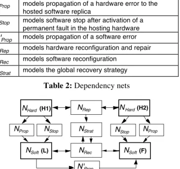
These dependencies are summarized in table 2 together with the names of the associated nets which are used to build up the high level model of the duplex system. The latter is given in figure 2 where NHard and

NSoft represent a computer and a software replica model

respectively.

NProp models propagation of a hardware error to the hosted software replica

NStop models software stop after activation of a permanent fault in the hosting hardware

N'Prop models propagation of a software error

NRep models hardware reconfiguration and repair

NRec models software reconfiguration

NStrat models the global recovery strategy Table 2: Dependency nets

NHard _(H1)

NSoft (F)

NRep

NRec

NStop

NProp NStrat NStop NProp

N'Prop

NSoft (L)

NHard (H2)

Figure 2: High level model of the duplex system

The corresponding GSPNs are built up following the rules and formal description presented in Sections 2 and 3; they are successively given in the remainder of the section.

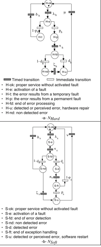
4.2. Hardware and software component nets

Figure 3 gives the component nets. The hardware model is based on the following assumptions:

• Faults are activated with rate λh.

• With probability ph the fault is permanent, (probability

of a temporary fault (1-ph)).

• The effects of an error due to a temporary fault are eliminated within a short time 1/δh.

• An error due to a permanent fault is either detected with probability d_h, or non detected (1-d_h); error processing rate: τh.

• The effects of a permanent, non detected error may be perceived later (perception rate ζh).

• The repair rate including software restart (following detection or perception of an error) is µ.

Equivalent assumptions are made regarding the behavior of the software replicas:

• Faults are activated with rate λs.

• An error is either detected with probability d_s, or non detected (1-d_s); detection rate τs.

• The detected error is processed by means of exception handling mechanisms during a short time 1/πs. At the

end of error processing, 1) if the fault is temporary (probability (1-ps)) its effects are eliminated and the

software resumes its normal mode of operation, 2) if the fault is permanent (probability ps); the software has

to be restarted (rate: ν) to eliminate its effects.(1-ps)

measures the efficiency of fault containment procedures [8, 11].

• The effects of a non detected error may be eliminated

(8)

H-ok λ_h δh H-e h p 1- p_h µ H-t h d 1-ζ_h H-nd H-p d_h H-u h τ H-fd

Timed transition Immediate transition • H-ok: proper service without activated fault • H-e: activation of a fault

• H-t: the error results from a temporary fault • H-p: the error results from a permanent fault • H-fd: end of error processing

• H-u: detected or perceived error, hardware repair • H-nd: non detected error

-a-_NHard λ_s S-ok δ_s ν S-e s τ S-fd d_s s d 1-s p 1-S-nd ζ_s p_s S-u S-d πs S-ft

• S-ok: proper service without activated fault • S-e: activation of a fault

• S-fd: end of error detection • S-nd: non detected error • S-d: detected error

• S-ft: end of exception handling

• S-u: detected or perceived error, software restart -b-_NSoft

Figure 3: Hardware computer and software replica nets

(elimination rate δs), or perceived (perception rate ζs)

in which case the software replica has to be restarted. The difference between these nets lies in that for hardware, temporary and permanent faults are differentiated by their respective consequences following activation, whereas for software, they can only be distinguished after specific processing [12].

4.3. Error propagation nets

From hardware to software: It is assumed that only

undetected errors and those due to temporary faults can

propagate from a hardware computer to the hosted software replica. The error propagation net, shown in figure 4, is initialized by the marking of place Prop following the firing of transition 1-dh (undetected error)

or of transition 1-ph (an error due to a temporary fault) in

the hardware net (initializing net). With probability 1-pph,

the error is not propagated and with probability pph it is. NProp is an action net, whose effects on the software net

(target net) are as follows:

• If the token is in S-ok, it is returned to S-e, the induced error is then processed in the same way as when the fault is activated without propagation (through λs in

figure 3-b).

• If the token is in S-e, since a fault is already activated in the software, the probability of error detection may be reduced (d's≤ds), if the errors are detected, the token

is returned to S-d; if they are non detected (with probability 1-d'_s) the token is returned to S-nd.

• If the token is in S-nd (an internal error is non detected in the replica) the propagated error and the internal error are detected with probability d"s (d"s≤d's, owing

to the perturbation due to the first error) the token is returned to S-d; the errors remain undetected with 1-d"s.

• If the token is in S-d the propagated error can compromise error processing and prevent the recovery of an error due to a temporary fault. The internal and propagated errors are recovered with probability 1-pp

(1-pp < 1-ps).

• If the token is in S-u, the software replica is already under restart, the token of NProp is absorbed through

tp-u and the token of NSoft is kept in S-u.

L (or F) net H1 (or H2) net pph Prop 1-p ph tp-ok Ps S-d tp-e _d' s 1-d' s tp-nd tp-d S-u p_p 1-p p tp-u d"s 1-d"_s h p 1-h d 1-P-nd P-d P-e S-ok S-e S-nd _N Soft NHard

Entry places and initializing arcs are indicated in bold

(9)

From L to F: The dependency net, the target net and the

effects on the target net are exactly the same but the initializing net is that of the software leader. It is assumed that only undetected errors in L and detected errors of L due to permanent faults, can propagate. The error propagation net is then initialized following the firing of 1-ds or ps. The probability of error propagation is pps.

At a higher modeling level, error propagation from L to F can be regarded as common mode failures.

4.4. Software stop and restart net

Following a detected error or the perception of an undetected error in an hardware computer, the hosted software replica is stopped and is restarted after repair of the hardware. We assume that the repair includes the replica restart. The software stop and restart net (Figure 5) is an action net, it is initialized by the marking of STP following the firing of transition ξh (perception of a non

detected error due to a permanent fault) or dh (detection

of an error due to a permanent fault). Transitions t1 to t5 remove the token from places S-ok, S-e, S-d, S-nd or S-u respectively. After repair of the hardware (including software restart), RST is marked and the token is returned to S-ok. RST STP S-ok S-d S-e S-nd S-u ζ dh tr t4 t1 t2 t3 t5 µ L (or F) net NSoft H1 (or H2) net NHard h

Figure 5: Software stop and restart, NStop

4.5. Hardware reconfiguration and repair net

As previously stated, we consider two different assumptions: A1 assumes a single repairman, while A2 assumes the presence of two repairmen. The corresponding nets are given in figure 6. Each net is composed of two parts corresponding respectively to reconfiguration (the shaded parts on the figures) and repair. They are grouped together because the reconfiguration is automatically followed by a repair. Since the reconfiguration strategy is the same, the associated nets are the same. The two nets are commented together and, when they are different, the figure number is specified.

NRep is initialized by the marking of H1F

(respectively H2F) following the firing of dh, detection of

an error due to a permanent fault or ζh perception of an

undetected error, in the hardware hosting L, H1 (respectively H2):

• if H1F is marked, H1 is in failure (H1 is the initializer, H2 the target):

- if H2 is not in failure (REP2 not marked) switching is attempted, (βh) and HSW is marked:

1) Switch can succeed with probability c_h, place SSW is then marked, REP1 REP2 H1F H2F SWH SSW EX1 EX2 FSW 2HF ch 1-ch βm βh H-ok H-u H-ok H-u t2h tf tex tex1 tex2 tr2 µ µ ζ dh (H1 net) NHard (H2 net) N_Hard h ζ d h h

-a- R1: with a single repairman

REP1 H1F H2F SWH SSW EX1 EX2 FSW ch 1-ch βm βh H-ok H-u H-ok H-u tex tex1 tex2 µ µ ERF t2f t1f ζ dh (H1 net) NHard (H2 net) NHard h ζ d h h

-b- R2: with two repairmen

Figure 6: Hardware reconfiguration and repair nets, NRep

2) It can fail with probability 1-ch, FSW is marked

and switching is done manually2_(β

m), SSW is

then marked; tex can be fired, places EX1, EX2 and REP2 are marked; tex1 and tex2 can be fired, they remove the token from H-u to H-ok, and from H-ok to H-u, F becomes the new leader, L the new follower and it can be restarted (REP2 is marked in figure 6-a for R1, H2F is marked in figure 6-b for R2),

2_{Other possible assumption: it can be assumed that the manual}

switch is not attempted. In this case, transition 1-ch leads to place

2HF (dashed arc in figure 6-a); place FSW and transition βm have

(10)

- for R1: if H2 is in failure (REP2 marked): t2h is fired removing the token from REP2 to 2HF; tr2 can then be fired returning a token in REP1 and one in H2F in order to repair H1, then H2, (for R2: if H2 is in failure (H2F marked): repair of H1 and H2 are enabled; at the end of H2 repair, if H1 is still under repair H2 is restarted with the leader),

• for R1 if H2F is marked: H2 is in failure (H2 is initializer and target): if H1 is not in failure (REP1 not marked), tf can be fired and REP2 is marked, authorizing the repair of H2; else the token stays in H2F until the end of H1 repair; repair of H2 in then allowed through the marking of REP2 (for R2: repair of H2 is enabled without any condition on H1).

For R1 and R2: if N_Repis initialed by H1 only, its is an action, activation and an authorization net; when initialized by H2 only, it is an authorization net. If itis initialed by H1 then H2 (or H2 then H1) it is an authorization net.

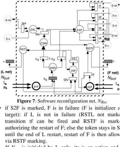
4.6. Software reconfiguration net

The software reconfiguration net is given in figure 7. It is initialized by the marking of S1F (respectively S2F) following the firing of transition ps, a detected error due

to a permanent fault or perception of an undetected error in L (respectively F):

• if S1F is marked, L is in failure (L is the initializer and F the target):

- if F is not in failure (RSTF not marked) switching is attempted (βs) and SWS is marked.

1) Switch can succeed with probability cs, places

EXL, EXF and RSTF are then marked. Marking of EXL allows firing of tex that removes the token from S-u to S-ok in L. Marking of EXF allows the firing of one of transitions t1 to t4 that removes the token in the leader net from places S-ok, S-e, S-d or S-nd and return it to S-u. Marking of RSTF enables transition v (in F) to restart it.

2) Switch can fail with probability 1-c_s, places EXF and 2SF are then marked. Marking of 2SF allows transition tr2 firing that marks places RSTL and S2F. Marking of place RSTL enables transition ν in the leader to restart it. Marking of S2F allows the follower restart only after the end of the leader restart.

- if F is in failure (RSTF marked) t2s is fired and 2SF is marked allowing the firing of tr2 that marks RSTL and S2F. Marking of place RSTL enables transition ν in the leader to restart it. Marking of S2F allows the restart of F only after the end of the leader restart.

ν ν S1F S2F SWS 2SF RSTF RSTL EXL EXF S-ok S-u S-ok S-d S-e S-nd S-u ps _ps bs t2s tf cs 1-cs tex tr2 t1 t2 t3 t4 CSW tex (L net) N_Soft (F net) NSoft ζs _ζs

Figure 7: Software reconfiguration net, NRec

• if S2F is marked, F is in failure (F is initializer and target): if L is not in failure (RSTL not marked) transition tf can be fired and RSTF is marked, authorizing the restart of F; else the token stays in S2F until the end of L restart, restart of F is then allowed via RSTF marking.

If N_Recis initialed by L only, its is an action and an authorization net. If N_Recis initialized by F only, it is an authorization net. If N_Recis initialed by L then F (or F then L) it is an authorization net.

4.7. Global recovery strategy net

The global recovery strategy net is initialized by NRep

through F1H following the firing of tex. If F is in failure (RSTF marked) t2 removes the token from RSTF and deposits a token in RSTL and another one in S2F in order for L to be repaired first. If F is not in failure (RSTF not marked) transition t1 deposits a token in CSW in order that the roles of the follower and leader to be exchanged. NStrat is an action net if place RSTF is marked and an

activation net if RSTF is not marked.

F1H SSW RSTL RSTF tex t1 t2 N_Rep N_Rec S2F

Figure 8: Global recovery strategy net, NStrat

4.8. Concluding remarks and global model

Due to lack of space the formal description of the previous nets is not presented. It can be checked that the hardware and the software GSPNs are live and bounded. With respect to dependency nets, verification of these

(11)

properties have to be done with the adjacent nets as indicated in figure 2, as follows

• N_Prop has to be validated connected with N_Hard and N_Soft, (N'_Prop is identical to N_Prop),

• N_Stop has to be validated with N_Hard and N_Soft, • N_Rep has to be validated with two N_Hard, • N_Rec has to be validated with N_Soft,

• N_Strat has to be validated with all the other nets (that have already been validated).

The overall model obtained by replacing the blocks of figure 2 with their GSPNs given in figures 3 to 8 has been processed by SURF-2. The marking graph has 1200 markings and the Markov chain 500 states without any state aggregation due to symmetry.

It could be argued that the state space may be very large for more complex systems, this is inherent to the complexity of the system to be modeled and to the level of detail considered. The only difficulty due specifically to our modeling approach is the number of markings; it can be overcome by using an aggregation technique at the GSPN level to suppress immediate (see e.g. [1]).

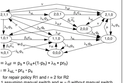
Considering again the duplex system, taking into account the fact that the transition rates associated with error detection and processing mechanisms are very high compared to failure, repair and restart rates (the durations of error detection and processing is of the order of the second whereas the intervals to failures are several hundreds of hours), the model can be reduced to 9 states as shown in figure 9. This model is to be considered as a limiting case allowing verification of the complete model in this specific case.

2,1,1 2,0,1 2,1,0 2,0,0 1,1,0 1,0,1 1,0,0 0,0,0 ν λsL λsF βs•cs λsLF ν λsL βs•cs λh•ph µ βh•ch βh•ch λh•ph λh•ph λh•ph λh•ph λsF λh•ph λsL m,0,1 w•βm µ r•µ λh•ph µ λh•ph λsL = λsF= ps • (λs+(1-ph) •λh • prh) λsLF= λsL • prs• ps

r = 1 for repair policy R1 and r = 2 for R2

w = 1 assuming manual switch and w = 0 without manual switch • 2,1,1: proper service of the computers, L and F

• 2,0,1: L is in failure • 2,1,0: F is in failure

• 2,0,0: both L and F are in failure

• 1,1,0: the computer hosting L is in failure • 1,0,1: the computer hosting F is in failure • 1,0,0: the compter hosting F, and L are in failure • m,0,1: failure of hardware switch, manual switch • 0,0,0: both computers are in failure

Figure 9: Reduced Markov chain of the duplex system

5. Conclusion

This work presented in this paper has allowed various types of dependencies between hardware and software components of a fault-tolerant system to be identified. These dependencies may result from functional or structural interactions as well as interactions due to reconfiguration and maintenance strategies. The dependability model of the system is obtained by composition of the components models with those associated with the dependencies. The rules for interfacing the models have been clearly defined and formally described to build up easily validable system models. The formal description facilitates the composition of the various GSPNs.

The modeling approach has been illustrated by a simple example, including all the types of dependencies identified: the duplex system. Modeling of this system showed the strong dependency between components. For example: the activation of a temporary hardware fault, may propagate an error to the hosted software component, which in turn may propagate to other components communicating with it (without being necessarily on the same computer). Thus the activation of a hardware fault, may lead to the restart of one or more software components. Even if this has already been observed on real-life systems, it has not been modeled explicitly in previous work. Also, we have shown how the modification of one or several assumptions can be performed without modifying all GSPNs, considering two repair policies and two switching policies (with or without manual switch).

The main advantage of the modeling approach, based on considering explicitly the interactions, lies in its efficiency for modeling several alternatives for the same system. These alternatives may differ by their composition (number of computers or replicas) or the organization (distribution of software components onto the hardware) or by the fault tolerance and maintenance strategies. One can clearly identify from the beginning the components and interactions that are specific and those that are common to all alternatives. The GSPNs that are common are thus developed and validated only once.

This approach has been applied to the French Air Traffic Control system (the subset associated with the Flight Plan Processing and Radar Data Processing) in [9] where twelve alternative architectures have been modeled and their unavailability compared to identify the most suitable one. Based on these results, additional and more detailed architectures have been modeled in [4]. This

(12)

application showed all the power of the modeling approach with the explicit modeling of the interactions.

Acknowledgments

The work presented in this paper has been partially supported by the French Civil Aviation Authority and SRTI SYSTEM while Marie Borrel was with SRTI SYSTEM and by the European Commission through the OLOS Network (A holistic approach to the dependability analysis and evaluation of control systems involving hardware, software and human resources).

References

[1] H. H. Ammar, Y. F. Huang and R. W. Liu, “Hierarchical Models for Systems Reliability, Maintainability, and Availability”, IEEE Trans. on Circuits and Syst., CAS-34 (6), pp. 629-38, 1987.

[2] G. Balbo, “On the Success of Stochastic Petri Nets”, in

6th International Workshop on Petri Nets and Per-formance Models, (Durham, NC, USA), pp. 2-9, 1995.

[3] C. Béounes, M. Aguéra, J. Arlat, S. Bachman, C. Bourdeau, J. E. Doucet, K. Kanoun, J.-C. Laprie, S. Metge, J. Moreira de Souza, D. Powell and P. Spiesser, “SURF-2: A Program for Dependability Evaluation of Complex Hardware and Software systems”, in 23rd

IEEE Int. Symp. Fault-Tolerant Computing, (Toulouse,

France), pp. 668-73, 1993.

[4] M. Borrel, Interactions between Hardware and Software

Components: Characterization, Formalization and Modeling — Application to CAUTRA Dependability,

PhD Dissertation, N°96-001, In French, 1996.

[5] A. Costes, C. Landrault and J.-C. Laprie, “Reliability and Availability Models for Maintained Systems Featuring Hardware Failures and Design Faults”, IEEE Trans. on

Computers, C-27 (6), pp. 548-60, 1978.

[6] J. B. Dugan and M. Lyu, “System-level Reliability and Sensitivity Analysis for Three Fault-tolerant Architectures”, in 4th IFIP Int. Conference on

Dependable Computing for Critical Applications, (San

Diego), pp. 295-307, 1994.

[7] W. R. Elmendorf, “Fault-tolerant Programming”, in 2nd

IEEE Int Symp. Fault-Tolerant Computing, (Newton,

Massashusetts), pp. 79-83, 1972.

[8] J. Gray, “Why Do Computers Stop and What Can be Done About it ?”, in 5th Int. Symp. on Reliability in

Distributed Software and Database Systems, (Los

Angeles, CA), pp. 3-12, 1986.

[9] K. Kanoun, M. Borrel, T. Moreteveille and A. Peytavin, “Modeling the Dependability of CAUTRA, a Subset of the French Air Traffic Control System”, in 26th Int.

Symp. Fault-Tolerant Computing (FTCS-26), (Sendai,

Japan), pp. LAAS-Report, 95-515, 1996.

[10] J.-C. Laprie, “Trustable Evaluation of Computer Systems Dependability”, in Applied Mathematics and Performance/Reliability Models of Computer/ Com-munication Systems, (Pise, Italie), pp. 341-60, 1983.

[11] J.-C. Laprie (Ed.), Dependability: Basic Concepts and

Terminology, Dependable Computing and Fault-Tolerant

Systems, 5, 265 p. , Springer Verlag, Wien-New York, 1992.

[12] J.-C. Laprie, “On The Temporary Character of Operation-persistent Software Faults”, in 4th Int. Symp.

on Software Reliability Engineering, (Denver, Colorado),

pp. 125, 1993.

[13] J.-C. Laprie and K. Kanoun, “X-ware Reliability and Availability Modeling”, IEEE Trans. on Software

Engineering, SE-18 (2), pp. 130-47, 1992.

[14] J.-C. Laprie, K. Kanoun, C. Béounes and M. Kaâniche, “The KAT (Knowledge-Action-Transformation) Approach to the Modeling and Evaluation of Reliability and Availability Growth”, IEEE Trans. Software

Engineering, SE-17 (4), pp. 370-82, 1991.

[15] J. K. Muppala, A. Sathaye, R. Howe, C and K. S. Trivedi, “Dependability Modeling of a Heterogeneous VAX-cluster System Using Stochastic Reward Nets”, in

Hardware and Software Fault Tolerance in Parallel Computing Systems (D.Avresky, Ed.), pp. 33-59, 1992.

[16] P. I. Pignal, “An Analysis of Hardware and Software Availability Exemplified on the IBM-3725 Communication Controller”, IBM Journal of Research

and Development, 32 (2), pp. 268-78, 1988.

[17] D. Powell, “Distributed Fault Tolerance: Lessons from Delta-4”, IEEE Micro, 14 (1), pp. 36-47, 1994.

[18] W. Sanders and J. Meyer, “Reduced Base Model Construction Methods for Stochastic Activity Networks”, IEEE Trans. on Selected Areas in

Communications, 9 (1), pp. 25-36, 1991.

[19] D. P. Siewiorek and R. S. Swarz, The Theory and

Practice of Reliable System Design, Digital Press, 1992.

[20] G. E. Stark, “Dependability Evaluation of Integrated Hardware/Software Systems”, IEEE Trans. on Reliability, R-36 (4), pp. 440-4, 1987.