Cardiac output estimation using arterial blood pressure waveforms

Cardiac Output Estimation using Arterial Blood Pressure

Waveforms

by

James Xin Sun

Bachelor of Science in Electrical Engineering and Computer Science (Massachusetts

Institute of Technology, 2005)

Submitted to the Department of Electrical Engineering and Computer Science

in partial fulfillment of the requirements for the degree of

Master of Engineering in Electrical Engineering and Computer Science

at the

MASSACHUSETTS INSTITUTE OF TECHNOLOGY

September 2006

@

James Xin Sun, MMVI. All rights reserved.

The author hereby grants to MIT permission to reproduce and distribute publicly

paper and electronic copies of this thesis document in whole or in part.

Author ...

Department of Electrical Engineering and Computer Science

September 1, 2006

Certified by...

. . . .

. . . w .. .

...

Roger G. Mark

Distinguished Professor in Health Sciences and Technology

Professor of Electrical Engineering

Thesis Supervisor

Accepted by ...

OCT 0

3 2007

... ... ...

Arthur C. Smith

Chairman, Department Committee on Graduate Students

Cardiac Output Estimation using Arterial Blood Pressure Waveforms

by James Xin Sun

Submitted to the Department of Electrical Engineering and Computer Science on September 1, 2006, in partial fulfillment of the

requirements for the degree of

Master of Engineering in Electrical Engineering and Computer Science

Abstract

Cardiac output

(CO)

determinant of global oxygen delivery. Historically, measurement of CO has been limited to critically-ill patients, using invasive indicator-dilution methods such as thermodilution via Swan-Ganz lines, which carry risks. Over the past century, the premise that CO could be estimated by analysis of the arterial blood pressure (ABP) waveform has captured the attention of many investigators. This approach of estimating CO is minimally invasive, cheap, and can be done continuously as long as ABP waveforms are available. Over a dozen different methods of estimating CO from ABP waveforms have been proposed and some are commercialized. However, the effectiveness of this approach is nebular. Performance validation studies in the past have mostly been conducted on a small set of subjects under well-controlled laboratory conditions. It is entirely possible that there will be circumstances in real world clinical practice in which CO estimation produces inaccurate results.

In this thesis, our goals are to (1) build a computational system that estimates CO using 11 of the established methods; (2) evaluate and compare the performance of the CO estimation methods on a large set clinical data, using the simultaneously available ther-modilution CO measurements as gold-standard; and (3) design and evaluate an algorithm that identifies and eliminates ABP waveform segments of poor quality.

Out of the 11 CO estimation methods studied, there is one method (Liljestrand method) that is clearly more accurate than the rest. Across our study population of 120 subjects, the Liljestrand method has an error distribution with a 1 standard deviation error of 0.8 L/min, which is roughly twice that of thermodilution CO. These results suggest that although CO estimation methods may not generate the most precise values, they are still useful for detecting significant (>1 L/min) changes in CO.

Thesis Supervisor: Roger G. Mark

Title: Distinguished Professor in Health Sciences and Technology Professor of Electrical Engineering

Acknowledgments

This research would not have been possible without the help and support of many people. First, I thank my thesis supervisor, Prof. Roger G. Mark. Your advice, support, care, and friendship are the reasons for the success of this thesis. Your leadership is truly inspiring. You have opened my eyes to the vast field of biomedical engineering, and I fully intend to pursue this field for the rest of my life.

I owe a great deal to Dr. Andrew Reisner and Mohammed Saeed. They introduced me

to the area of cardiac output estimation. Their help and support unquestionably shaped the scope of my research.

I thank all members of the Lab for Computational Physiology and members of the BRP. It is because of them I enjoyed being at the lab almost every day. Thanks to Dr. Gari Clifford for all the signal processing advice and his British sense of humor; to Dr. Thomas Heldt for his technical advice and of course, for his self-confident attitude; to Tushar Parlikar for keeping this final semester so entertaining; to Mauricio Villarroel, the UNIX guru, for the database and Linux support; to Anton Aboukhalil for his magic tricks.

I thank all my friends at MIT. Dearest thanks to every member of the "little-family"

for all those get-togethers and birthday showerings: I will treasure all those memorable moments; to Tin, the "free electricity" Burmese, for being a great friend and lab-mate at LCP.

I sincerely thank my family (mom, dad, Andrew) for all their encouragement, love, and support.

This work was made possible by grant R01 EB001659 from the National Institute of Biomedical Imaging and Bioengineering.

Contents

1 Introduction 13

1.1 M otivation . . . . 13

1.1.1 Measurement of cardiac output . . . . 13

1.1.2 Estimating cardiac output from arterial blood pressure . . . . 16

1.1.3 MIMIC II database & data quality . . . . 16

1.2 T hesis goals . . . . 17

1.3 Thesis outline . . . . 17

2 Cardiac Output Estimation Theory 19 2.1 Lumped parameter methods . . . . 20

2.1.1 Mean arterial pressure . . . . 20

2.1.2 Windkessel model [5] . . . . 20

2.1.3 Windkessel RC decay [4] . . . . 21

2.1.4 H erd [7] . . . . 21

2.1.5 Liljestrand nonlinear compliance [12] . . . . 21

2.2 Pressure-area methods . . . . 21

2.2.1 Systolic area [19] . . . . 22

2.2.2 Systolic area with correction [19, 10] . . . . 22

2.2.3 Systolic area with corrected impedance [21] . . . . 22

2.2.4 Pressure root-mean-square [9] . . . . 22

2.3 Lumped-parameter, instantaneous flow methods . . . . 24

2.3.1 Godje nonlinear compliance [6] . . . . 24

2.3.2 Wesseling Modelflow [20] . . . . 25

2.4 Limitations of CO estimation . . . . 25

3 Signal Abnormality Indexing 27 3.1 Introduction . . . . 27 3.2 Methods ... ... ... 27 3.2.1 Feature extraction . . . . 29 3.2.2 Abnormality indexing . . . . 29 3.2.3 Algorithm evaluation . . . . 30 3.3 R esults . . . . 32

3.3.1 SAI versus human . . . . 32

3.3.2 Sensitivity analysis . . . . 32

3.3.3 Cardiac output estimation error . . . . 33

4 Evaluation Methods 35

4.1 Data extraction . . . . 36

4.2 Implementation of CO estimators . . . . 36

4.2.1 ABP beat detection . . . . 36

4.2.2 ABP feature extraction . . . . 37

4.2.3 CO estimator implementation . . . . 38

4.2.4 Signal quality and bad beats elimination . . . . 38

4.2.5 Running-average LPF to reduce beat-to-beat fluctuations . . . . 40

4.3 Comparing estimated CO to gold-standard CO . . . . 40

4.3.1 Averaging beat-to-beat CO estimates . . . . 41

4.3.2 Calibration techniques . . . . 41

4.3.3 Relative CO estimation . . . . 42

4.4 Error analysis . . . . . . . . 43

5 Results and Discussion 47 5.1 Subject population statistics . . . . 47

5.2 Removal of poor quality waveforms . . . . 47

5.3 Absolute CO estimation . . . . 49

5.4 Variability of calibration constants . . . . 53

5.5 Variability of CO estimates . . . . 53

5.6 Relative CO estimation . . . . 54

5.7 Error analysis of selected CO estimators . . . . 54

5.8 Selected time series case studies . . . . 60

5.9 D iscussion . . . . 60

6 Conclusions and Future Research 63 6.1 Sum m ary . . . . 63

6.2 Suggestions for future research . . . . 64

A Notation Summary 65 B Selected Code Descriptions 67 B .1 w avex.m . . . . 67 B .2 trendex.m . . . . 67 B .3 w abp.m . . . . 68 B.4 abpfeature.m . . . . . 68 B .5 jSQ I.m . . . . 68 B.6 estimateCO.m . . . . 69

List of Figures

1-1 Cardiovascular system. . . . . 14

1-2 Indicator dilution principle. . . . . 15

1-3 ABP waveform. . . . . 16

1-4 Cardiovascular system. . . . . 17

2-1 Mean arterial pressure Pm and cardiac output

Q.

2-2 The Windkessel RC circuit model. . . . . 20

2-3 Windkessel model with nonlinear capacitor. . . . . 22

2-4 Arterial tree of a dog. . . . . 23

2-5 A transmission line circuit. . . . . 23

2-6 Pressure-area during systole. . . . . 24

2-7 Godje model with nonlinear capacitance and aortic impedance terms. . . . 24

2-8 Wesseling's modelflow model. . . . . 25

2-9 Pressure waveforms in aorta versus radial artery. . . . . 25

3-1 Damped ABP waveform. . . . . 28

3-2 ABP waveform with disturbance. . . . . 28

3-3 Noisy ABP waveform. . . . . 28

3-4 Example of SAI . . . . 29

3-5 SAI block diagram. . . . . 29

3-6 SAI parameter sensitivity. . . . . 32

3-7 CO estimation error as a function of maximum accepted cSAI . . . . 34

4-1 A system for evaluating CO estimation performance. . . . . 36

4-2 Data flow diagram for CO estimation. . . . . 36

4-3 The slope sum function . . . . 37

4-4 Ps, Pd, and P detection . . . . 38

4-5 The cardiac cycle. . . . . 39

4-6 End of systole and systolic area . . . . 39

4-7 Beat-to-beat variability in ABP waveform. . . . . 40

4-8 Window size for averaging CO estimates. . . . . 41

4-9 Vector visualization of TCO and estimated CO . . . . 42

4-10 Bland-Altman plot . . . . 43

4-11 Percentage changes in TCO versus estimated CO . . . . . 45

5-1 Population statistics . . . . 48

5-2 Bland Altman plot . . . . 50

5-3 Bland-Altman error analysis plots. . . . . 51

5-5 Performance of percentages changes in CO. . . . . 55

5-6 Performance of percentages changes in CO (continued). . . . . 56

5-7 CO estimation (Liljestrand) error as functions of several variables. . . . . . 57

5-8 CO estimation (MAP) error as functions of several variables (MAP). ... 58

5-9 CO estimation (Modelflow) error as functions of several variables. . . . . 59

5-10 Time series of caseID 8463 using the Liljestrand CO estimator. . . . . 61

List of Tables

2.1 Cardiac output estimators . . . . 19

3.1 ABP features . . . . 30

3.2 SA I logic . . . . 30

3.3 CO estimators taken from Table 2.1. . . . . 31

3.4 SAI versus human: distribution . . . . 32

3.5 SAI versus human: statistical summary . . . . 32

3.6 SAI sensitivity . . . . 33

4.1 ABP features . . . . 37

5.1 Population statistics . . . . 47

5.2 Estimation error in L/min at 1 SD with 3 different calibration methods. . . 49

5.3 Variability of k for Cl and C3 calibration. . . . . 53

5.4 Variability of CO estimates. . . . . 53

5.5 Relative CO estimation error. . . . . 54

A.1 Commonly used acronyms and symbols . . . . 65

C.1 p-values using the Kolmogorov-Smirnov test. . . . . 71

Chapter 1

Introduction

1.1

Motivation

The cardiovascular system provides vital nutrients and removes wastes from body tissues. The powerhouse of the cardiovascular system is the heart, pumping out oxygenated blood to the systemic circulation (Figure 1-1). For a normal healthy adult at rest, cardiac output

(CO), the average flow rate of blood pumped into the aorta, is approximately 5 liters

per minute. For an Olympic athlete at maximum workout, CO exceeds 30 L/min. For a patient in circulatory shock, CO can be less than 2 L/min. The tremendous dynamic range suggests that CO is a key indicator of one's hemodynamic state. Thus, it would be a tremendous asset to determine CO accurately, reliably, and continuously using minimally invasive methods.

1.1.1 Measurement of cardiac output

Flowmeter. The most direct and accurate way of measuring CO is to use a flowmeter. One could conceivably place an ultrasonic flow probe around a major vessel protruding from the heart such as the aorta. Instantaneous pulsatile flow is obtained with a millisecond time resolution. Stroke volume, the volume of blood ejected into the aorta per cardiac cycle, is calculated by integrating the flow curve over a cardiac cycle. CO is then obtained by multiplying stroke volume with heart rate. Unfortunately, this direct flow measurement requires thoracotomy (surgical incision of the chest wall), which is impractical to perform in humans just for diagnostic purposes.

Fick principle. A more practical way to obtain CO is through the Fick principle of

02 mass balance. It states that the amount of 02 consumed must equal the difference in 02 quantity between the arterial and venous circulation. Using this fact, CO is obtained as

follows:

CO a02 consumption [L 02/min]

arterial 02 content - mixed venous 02 content [L 0 2/L blood]

Therefore, to determine CO, 02 consumption and content in blood need to be measured. Thermodilution. Another clinically plausible method of obtaining CO is through an indicator dilution technique, which is based upon conservation of the indicator solution.

As shown in Figure 1-2, cardiac output

Q

Head

X

Trunk, arms

Veno covo

SpUMc

PV

portal

Mesenteric

Kidney

Tubuaer

Gaeu

Hepoitc, eqs

F

W

Figure 1-1: The cardiovascular system. Figure adapted from [13]. A

I

I

a.

A

SronehiW

Lung$

x----Aor

ta---Cot

ay

downstream at point B. By dye conservation, the amount injected must pass through point B, and CO is obtained as follows:

CO = [mg]

f t2c(t)dt [mg-min/(L blood)]

Clinically, the most popular indicator dilution technique is thermodilution, in which cold saline of precisely known volume and temperature is injected, and then the temperature profile is measured downstream.

Mixer QA q mg c~eLcunp, Phokmcell inje*d WD Densitmeter t2 Time

Figure 1-2: Indicator dilution principle. Figure adapted from [2].

Doppler ultrasound. More recently, a completely noninvasive method known as

doppler ultrasound has been developed to measure CO [8]. This technique measures the aorta's instantaneous blood flow velocity v(t) and cross sectional area A. Then stroke volume can be calculated by integrating v(t) over a cardiac cycle of duration T:

SV = Aj v(t)dt

Remarks. Although the Fick method and thermodilution are both clinically feasible, they are still quite invasive and can only be performed in well-equipped environments like intensive care units (ICUs) and cardiac catheterization labs. Measurement of mixed venous 02 requires a blood sample from the pulmonary artery. Injection of cold saline must be into a major vessel through which the entire CO flows. Consequently, a Swan-Ganz catheter that is threaded through the vena cava, through the right heart, and into the pulmonary artery is used to facilitate thermodilution CO measurements. Doppler ultrasound, while completely noninvasive and reasonably accurate, is expensive. Running this device requires costly equipment and an expert technician. In addition, none of the methods discussed in this section are practical for continuous bedside monitoring of a patient's CO.

1.1.2

Estimating cardiac output from arterial blood pressure

Throughout the past century, the premise that CO could be estimated by analysis of the arterial blood pressure (ABP) waveform (Figure 1-3) has captured the attention of many investigators. More than a dozen methods of calculating CO from ABP have been proposed, many of which are now commercially available. This approach to determine CO has the following advantages:

" Obtaining ABP is non-invasive or minimally invasive.

" ABP waveforms are routinely measured in clinical settings such as ICUs.

" The ABP waveform is measured continuously, allowing for continuous CO estimates. " Cost benefits: The transformation from ABP to CO requires only numerical

compu-tation. No expensive equipment or expert technicians are required.

O100 80 60 40 -0 0.5 1 1.5 2 2.5 3 time [sec]

Figure 1-3: The arterial blood pressure (ABP) waveform.

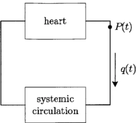
To understand the relation between pressure (ABP) and flow (CO), we first start with a very simple representation of the cardiovascular system. Shown in Figure 1-4, there are two blocks: the heart and the systemic circulation. Blood flows out of the heart with a rate of q(t) and a corresponding arterial pressure P(t). Assuming that the internal state of the heart and the systemic circulation does not change, then it is plausible that higher flow corresponds to higher pressure. Unfortunately, in real life, system states such as systemic resistance can dynamically change within seconds, giving rise to a much more complicated pressure-flow relationship. The dozen or so methods of determining flow from pressure use cardiovascular system models and represent the internal structure of the two blocks in Figure 1-4 with varying levels of complexity, thereby quantitatively relating P(t) and q(t). Having so many different P - q relations existing today suggests that there is no

con-sensus as to which method works best. Studies conducted in the past have mostly been on animals or a small set of human subjects under well-controlled laboratory conditions. The

CO estimators have not been extensively evaluated with a large set of clinical ABP

wave-forms, hence the performance of CO estimation is still uncertain. It is entirely possible that there will be circumstances in real world clinical practice in which these indirect methods produce unacceptable estimates. The main goal of the research presented in this thesis is to determine the performance of the CO estimators.

1.1.3 MIMIC II database & data quality

Before evaluating the performance of CO estimation, we must first establish a suitable study population that contains ABP waveform data and contemporaneous reference CO

heart P(t)

q(t)

systemic circulation

Figure 1-4: A simple, lumped cardiovascular system. The heart nourishes the systemic circulation with blood at flow rate q(t) with arterial pressure P(t).

measurements (along with other pertinent clinical details such as patient age, presence or absence of valve disease, etc.). The Multi-parameter Intelligent Monitoring for Intensive Care II (MIMIC II) database [16] is the product of an initiative by the MIT Laboratory for Computational Physiology (LCP) to create a massive, temporal database to facilitate the research and development of an Advanced Patient Monitoring System. Currently, this database has physiologic waveform data from over 3500 ICU patients hospitalized at Beth Israel Deaconess Medical Center, Boston, USA.

Prom this database, we identified 120 patients with simultaneously available ABP wave-forms (125-Hz sampled) and thermodilution CO measurements. Since MIMIC II data is collected in a far less controlled environment than a typical research laboratory setting, ABP waveforms are prone to corruption, causing CO estimators to generate bizarre outputs. To address this problem, an algorithm that identifies and rejects bad waveform segments is required.

1.2

Thesis goals

The research presented in this thesis aims to achieve the following:

" To study the principles of CO estimation from ABP waveforms and build a

compu-tational system that estimates CO using 11 of the established methods.

" To evaluate and compare the performance of the CO estimation methods on a large set

clinical data from the MIMIC II database and determine whether the CO estimation is useful for clinical use.

" To design and evaluate an algorithm that quantifies ABP waveform quality.

1.3

Thesis outline

This thesis is divided into six chapters and two appendices.

Chapter 2, Cardiac Output Estimation Theory, explains the principles of the 11 different methods we study for CO estimation. Physiologic principles and theory from electrical

circuits are used whenever appropriate to provide intuition. Limitations of CO estimation are also discussed.

Chapter 3, Signal Abnormality Indexing, addresses the key issue of ABP waveform quality. CO estimation relies on a clean ABP waveform, in which pressure and temporal features may be reliably obtained. This chapter discusses the design and evaluation of an algorithm that flags poor quality ABP waveforms.

Chapter 4, Evaluation Methods, explains the computational system built to evaluate CO estimation, which involves database extraction, ABP waveform processing, CO estimator implementation, and performance evaluation.

Chapter 5, Results and Discussion, reports the performance of CO estimation. We discuss subset error analysis to determine the physiologic situations in which CO estimators are likely to be more erroneous.

Chapter 6, Conclusions and Future Research, summarizes the important findings from this research and suggests possible areas worthy of further exploration.

Appendix A presents a table summarizing the acronyms and mathematical notations used throughout this thesis. Appendix B contains input/output relations of important MATLAB source code to help elucidate Chapter 4.

Chapter 2

Cardiac Output Estimation Theory

In the cardiovascular system, the relationship between arterial blood pressure (ABP) and cardiac output (CO) is quite complex. Over a dozen methods of estimating flow from pres-sure have been proposed. Most of the methods operate at a beat-by-beat time resolution, calculating the stroke volume of each beat. Then, CO is calculated by multiplying stroke volume with heart rate. The bases of these methods are models of the systemic circulation. Table 2.1 lists the 11 CO estimators studied in this thesis. (Several CO estimators are not studied because (1) the algorithms described in publications were unclear or (2) they are too similar to one of the 11 estimators in Table 2.1.) All expressions given in the table are proportional to CO. The proportionality constant encapsulates terms such as arterial compliance and peripheral resistance that are not obtainable from a given model. The first

5 methods are based on lumped-parameter circuit models of circulation. The next 4 are

based upon distributed transmission line models. The last 2 are lumped circuit models with ability to produce instantaneous flow waveforms, which becomes CO when time-averaged.

Table 2.1: Cardiac output estimators

CO estimator

Mean arterial pressure Windkessel [5]

Windkessel RC decay [4] Herd [7]

Liljestrand nonlinear compliance [12]

CO = k - below Pm

PP -

In

f

Systolic area [19] As. f

Systolic area with correction [19, 10] (1+ A) A

f

Systolic area with corrected impedance [21] (163 +

f

Pressure root-mean-square-simplified form of [9] ((P(t) - Pm)2) f

Godje nonlinear compliance [6] complex formula

Wesseling Modelflow [20] nonlinear, time-varying model

2.1

Lumped parameter methods

2.1.1

Mean arterial pressure

In the simplest model, the heart is represented as a current source and systemic circulation as a resistor (Figure 2-1). This circuit analogy is only appropriate for time-averaged flow, not pulsatile flow. Given mean arterial pressure and systemic resistance, CO may be computed via Ohm's law as follows:

Pm

Q

=R

+

Q {R Pm

Figure 2-1: Mean arterial pressure Pm and cardiac output

Q.

2.1.2

Windkessel model [5]

The arteries are capable of storing blood. Even with zero transmural pressure across the arterial walls, approximately 500ml of blood can reside inside the arterial system for a nominal person. At a mean arterial pressure of 100mmHg, 700ml of blood are in the arteries [13]. Therefore, it is sensible to represent the arteries as a capacitor (Figure 2-2). This model is the Windkessel model.

q(t) P(t)

q(t) R C P(t)

LL

t

LTdt

Figure 2-2: The Windkessel RC circuit model. The heart is modeled as a flow source q(t) with impulse train ejections. Systemic circulation is modeled with arteriolar resistance R and arterial compliance C. The ABP waveform P(t) generated has an infinitesimally short systolic duration followed by exponential decay during diastole.

One major "upgrade" in the Windkessel model is in its ability to capture the pulsatility of the cardiovascular system. The current source, now as an ideal pulsatile pump, generates a periodic impulse train, which gives rise to the ABP waveform P(t). From circuit theory, it can be shown that in steady state, stroke volume is proportional to the amplitude of the

ABP waveform (P, - Pd) and arterial capacitance. Thus, CO is given as:

2.1.3

Windkessel RC decay [4]

If the time constant r of the Windkessel RC circuit model is known, then cardiac output may be computed in another way:

Pm Pm Pm

Q=P-=C-P

_R

=C-P

There are several methods to determine -r:

* Use the Windkessel idealization that ejection is instantaneous. This way, the entire cardiac cycle is in exponential decay from systolic to diastolic pressure. Mathemati-cally,

Pd = Pe-Tl

where T is the beat period. Solving for r, we obtain:

T

In

n

Pd

Hence, the final CO expression:

PM Ps

Q

-P-T Pd

" Perform a least squares fit of an exponential decay to the diastole portion of the ABP waveform. Then, the best-fitted r is obtained.

" Use a refined exponential fitting technique by Mukkamula et al. [14]. In this thesis, r is obtained separately using the first two methods.

2.1.4

Herd [7]

The Herd method proposes that stroke volume is proportional to Pm-Pd. This methodology is based upon empirical evidence and no physiologic intuition is given [7].

2.1.5

Liljestrand nonlinear compliance [12]

Arterial capacitance is not constant but varies as a function of pressure. As arterial pressure increases, arterial walls stiffen, reducing capacitance. From the Windkessel model point of

view, the Liljestrand and Zander method takes into account the nonlinearity using C =

kSP (Figure 2-3). Hence, CO becomes:

k

Q

=

-

P-f

Ps + Pd

2.2

Pressure-area methods

One major problem with lumped parameter models is that the arterial tree is really a distributed, not lumped system (Figure 2-4). In theory, the arterial tree could be more

q(t) R C P(t)

Figure 2-3: Windkessel model with nonlinear capacitor. Liljestrand and Zander propose

that C oc (P + P)-'.

accurately modeled using the transmission line circuitry, which captures the distributed nature and associated effects such as impedance and wave reflections. Although none of the pressure-area methods are explicitly derived from transmission line circuit theory, the arterial tree is approached from a distributed system point of view.

2.2.1 Systolic area [19]

One key observation made from the distributed arterial tree is that stroke volume is pro-portional to the area under the systole region (A,) of the ABP waveform (Figure 2-6). CO becomes:

Q

2.2.2 Systolic area with correction [19, 10]

First appearing in Warner et al. [19], a (1

+

previous CO estimation method. This factor is probably compensating for the fact that the duration of systole, T, is not a negligible fraction of the beat period, thereby causing outflow from the capacitor to the resistor. The exact physiologic rationale is unexplained.

CO estimate with this correction factor becomes:

Q= k - 1+ T As. f

Td

2.2.3 Systolic area with corrected impedance [21]

Wesseling et al. [21] introduced another correction factor based upon empirical evidence and optimal regression analysis. With the corrected impedance factor, CO becomes:

Q

f

f

2.2.4 _{Pressure root-mean-square [9]}

An adaption of LiDCO's CO method [9], stroke volume is thought to be proportional to the

square of each cycle in the ABP waveform. From AC circuit theory, root-mean-square of an AC voltage waveform is proportional to power. Thus, this method believes that stroke volume and AC power of the ABP waveform are linearly related. Thus, CO becomes:

Q

Figure 2-4: Arterial tree of a dog. In reality, the arterial tree is more accurately modeled

by transmission lines rather than lumped parameter model. Figure adapted from [15].

---Figure 2-5: A transmission line circuit. The elementary component is enclosed by the dashed box. The transmission line is a series of elementary components. With the inductor-capacitor pairing, pulse wave propagation is generated.

Figure 2-6: Pressure-area during systole. One cycle of the ABP waveform is shown. Stroke volume is believed to be proportional to the area of the shaded region. Figure adapted from

[10].

2.3

Lumped-parameter, instantaneous flow methods

Two of the CO estimation methods investigated in this thesis use lumped parameter models to calculate the instantaneous pulsatile flow, q(t), from ABP waveforms. Once q(t) is obtained, then beat-to-beat CO is the time-averaged flow over a cardiac cycle:

Q=

2.3.1 Godje nonlinear compliance [6]

Godje's cardiovascular system model is shown in Figure 2-7. Compared to the Windkessel model, an aortic impedance element, Z, is added, and the heart becomes a pressure source rather than a flow source. Also, arterial compliance is nonlinear. The expression for arterial compliance is optimized to minimize mean square error of the flow (derivation for the optimization is not given in the paper):

p3

C = _t)

R - (dP(t)/dt) ' 3PP(t) - 3P-P

Using Kirchhoff's current law, instantaneous flow is obtained:

P(t) ) dP =1 _t)_+_m_____ P dP(t)/dt

R dt R 3PmP(t) - 3Pm - P(t)2 (dP(t)/dt)

Z

R C

q(t)

2.3.2

Wesseling Modelflow [20]

Wesseling's modelflow method is one of the most complex (Figure 2-8). The circuit is

similar to Godje's but with every circuit element becoming nonlinear. Aortic impedance is a function of arterial compliance; arterial compliance is a function of pressure; systemic resistance is a function of pressure divided by flow. The nonlinear relationship between C and P(t) are based from Langewouters et al.'s [11] regressions.

P(t) + R C

q(t)

Figure 2-8: Wesseling's modelflow model.

2.4

Limitations of CO estimation

The 11 methods of estimating CO from ABP waveforms have several limitations. First, all methods require at least one calibration to obtain absolute CO values in liters per minute. Without calibration from a CO measurement such as thermodilution, one can only obtain relative estimates, which are still beneficial to the clinicians, especially if CO changes by a substantial fraction in a given patient.

The cardiovascular models used to estimate CO are vastly simplified from reality, even for the most complex ones. First, although the pressure-area under systole methods are based upon the distributed arterial tree, the theoretical foundations are not firmly estab-lished [19, 10]. It would be beneficial to derive an expression for CO from transmission line theory. Second, many of the methods assume that a central ABP waveform (such as one from the aorta) is used. Clinically, radial ABP waveforms are by far more popularly measured. Figure 2-9 shows that there is a substantial difference between ABP waveforms in aorta versus radial arteries, though there are models that attempt to estimate the aor-tic waveform using the radial artery waveform. Lastly, systolic area calculations require detecting the end of systole, which is completely nontrivial in radial ABP waveforms. In aortic ABP, the dicrotic notch signifies the end of systole. In radial ABP, the dicrotic notch is masked by wave reflections and high frequency signal attenuation.

150 - Radial

1::

F

50

-Figure 2-9: Pressure waveforms in aorta versus radial artery. Notice that systolic pressure in the radial artery tends to be higher than that of the aorta. Figure adapted from [15].

For several reasons, the more complex methods may perform worse than the simpler ones. First, due to corruption susceptibility of the ABP waveform, especially in a clinical setting, complex methods may falter if a particular ABP feature is corrupt. The simplest method, CO is proportional to mean arterial pressure, is by far most robust to noise because of its averaging nature. Second, the more complex methods have more circuit components. Wesseling's modelflow method determines the value of each component through ABP wave-forms and regressions using age and gender. Regression lines were determined from a very small population (less than 50), which may not be representative of the entire human pop-ulation. Therefore, modelflow may only perform well on patients with similar physiology to Wesseling's small study population.

A fundamental limitation of CO estimation performance is due to ABP waveform quality.

Features and morphology of the ABP waveform need to be clean, especially for the more complex CO estimation methods. Thus, CO estimation is likely to fail in patients with intra-aortic balloon pumps, valve regurgitation diseases, and long-lasting arrhythmias such as atrial fibrillation.

Further discussion on the limitations of CO estimation can be found in an editorial by Lieshout and Wesseling [18].

Chapter 3

Signal Abnormality Indexing

3.1

Introduction

Cardiac output (CO) estimation from arterial blood pressure (ABP) waveforms rely on a clean ABP waveform, in which beat-to-beat features such as mean pressure, duration of systole, and beat period may be reliably obtained. Noisy, artifactual, damped, and irregular (not sinus rhythm) ABP waveforms may easily lead to bizarre CO estimates. Figures 1, 3-2, 3-3, 3-4 show examples of clinical ABP waveforms from MIMIC II in which CO estimates are likely to fail. Therefore, it is important to design an algorithm that can flag anomalous beats in the ABP waveform (Figure 3-4). We define a beat as anomalous when any feature in the beat becomes obscured. Median filtering helps to reduce some sporadic anomalies, but fails as anomalies become more frequent.

In this chapter, we present the signal abnormality index (SAI). The algorithm outputs at a beat-level time resolution and intelligently detects abnormal beats by imposing a series of constraints on physiologic, noise/artifact, and beat-to-beat variability. SAI does not distinguish between anomalies arising from physiologic disturbances such as an arrhythmia and non-physiologic phenomena such as noise.

The SAI algorithm was evaluated on clinical ABP waveforms of 120 patients from MIMIC II (see Section 1.1.3). Using the 120 records, we quantified the performance of the SAI algorithm in 3 ways: comparing the algorithm's performance to a human expert, analyzing the sensitivity of the algorithm's output, and determining whether cleaner wave-form segments yield better CO estimates.

3.2

Methods

Figure 3-5 shows an overview of the SAI algorithm. First, a beat detection algorithm [22] marks the onset of each beat. The onset markers allow for feature extraction at beat-level resolution. For each beat, features such as heart rate, systolic blood pressure, diastolic blood pressure are obtained. Features are then evaluated by a series of abnormality criteria, which check for noise level, physiologic ranges, and beat-to-beat variations. The output of each abnormality criterion is binary, '0' for no flag (clean beat) and '1' for flag. Finally, the outputs of all abnormality criteria are combined via the logical OR operation.

-b 150 100 K50 0 5 10 15 20 time [min] 150 150 100 100 50 50--0 1 2 3 4 5 0 1 2 3 4 5

time [sec] time [sec]

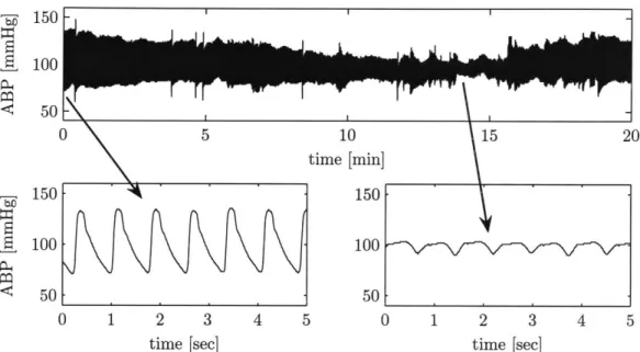
Figure 3-1: Damped ABP waveform. Top plot shows a 20 minute ABP waveform. Bottom-left plot is a zoom-in near the earlier part, and bottom-right plot is a zoom-in around the 14th minute. Damping caused the pulse pressure to decay from 60mmHg to 10mmHg.

*-

50 -

-0 2 4 6 8 10

time [sec]

Figure 3-2: ABP waveform with disturbance. Beat detection becomes nontrivial and un-predictable here, giving rise to inaccurate CO estimates. (Upon closer examination of the patient record, this waveform segment was from a patient who had an 2-to-1 intra-aortic balloon pump, which generated the middle beat for each group of 3 beats shown.)

'6 200

100

0 2 4 6 8 10

time [sec]

Figure 3-3: Noisy ABP waveform. Noisy beat-to-beat features give rise to inaccurate CO estimates, especially for the more complicated CO estimators.

TEF 150 -100 50 -0 0 5 10 15 20 25 time [seconds]

Figure 3-4: ABP waveform with artifacts. Corruption in the first 15 seconds is likely due to improper catheterization caused by movement. Corruption in 20-22 seconds is likely a motion artifact. Signal abnormality index (SAI) is shown on bottom, raising a flag in regions of abnormality.

sequence of length

n.

n Y = fraction of flagged beats = nEy[k)

k=1

where y[k] is the SAI of the k-th beat. cSAI, with a continuous domain of 0 < Y < 1, is

a useful measure of the abnormality of an entire waveform segment. (e.g. a segment of 50 beats with 4 flagged would yield a cSAI of 0.08.)

The rest of this section explains several components of the SAI in detail and proposes methods for algorithm evaluation.

ABP - Beat ABP _*detection Abnormality criterion 1 Feature _Logical .. 11.. -> extraction OR - .11 . Abnormality_ criterion N

Figure 3-5: SAI block diagram. Input is an ABP waveform. Output is a binary string, assigning a value (no flag=0, flag=1) to each beat in the ABP waveform.

3.2.1 Feature extraction

The feature extraction algorithm obtains a set of features shown in Table 3.1. For each beat, P, and Pd are the local minimum and maximum around the pressure onset point. Pm is the average pressure between adjacent onsets. T is the time difference between adjacent onsets. Noise level is defined as the average of all negative slopes in each beat.

3.2.2 Abnormality indexing

With blood pressure features available, the SAI algorithm is ready to interpret them. Table

Table 3.1: ABP features Feature Description

PS Systolic blood pressure

Pd Diastolic blood pressure

P, Pulse pressure (P, - Pd)

Pm Mean arterial pressure

T Duration of each beat

f Heart rate (60/T)

w noise: mean of negative slopes

Feature PS Pd PM

f

-Pd[k]

1

Table 3.2: SAI logic

Abnormality criteria P > 300 mmHg Pd < 20 mmHg Pm < 30 or Pm > 200 mmHg

f

f

The first 5 criteria in Table 3.2 impose bounds on the physiologic ranges of each feature. For example, any beat with a diastolic pressure of less than 20mmHg is flagged.

The 6th criterion is the noise detector. With high frequency noise, there will be large negative slopes in the waveform. Based upon this observation and by inspecting ABP data, we decided that any beat with a mean negative slope less than -40mmHg/1OOms is flagged. Note that this noise detector is not useful for identifying low frequency noise such as baseline wander.

The final 3 criteria compare ABP features between adjacent beats. Large sudden changes in beat-to-beat features are likely indications of abnormality. For example, if the (k - 1)-th systolic pressure and the k-th systolic pressure differs more than 20mmHg, then the k-th beat is flagged.

3.2.3 Algorithm evaluation

Using 120 patient records from the MIMIC II database, the SAI algorithm was evaluated in 3 ways:

1. Compare the algorithm's performance to a human expert in detecting anomalies in

ABP waveform segments. Ideally, the algorithm should be in perfect concordance with the human.

2. Analyze the sensitivity of algorithm's output to perturbations of each threshold pa-rameter in Table 3.2. A robust algorithm would be relatively insensitive to such perturbations.

3. Determine whether cleaner waveform segments, as indicated by low cSAI values, yield

better CO estimates.

In comparing to a human expert annotator, 246 ABP segments were randomly selected, each 10 seconds long. For each segment, the SAI algorithm outputs '1' if any beat is flagged as abnormal, '0' otherwise. Similarly, the human identifies any abnormality and classifies each segment using the following convention:

-- No irregularity-regular, homogeneous beats with negligible artifacts and

noise.

-+ Minor irregularity-clean waveform with minor timing irregularity of

beats and/or minor artifacts. Key morphologic features are still clearly identifiable.

±- Irregularity present-all beats similar, but one beat stands out from

oth-ers with timing or shape, and/or artifact present obscuring a portion of a beat.

++ Major irregularity present-more than one beat patently dissimilar from

other beats, and/or artifact present completely obscuring key features of beats.

Notice that human annotations have 2 gray zones (-+ and +-), which are used when the

waveform's abnormality is not completely obvious.

For sensitivity analysis, the abnormality criteria are tested independently of each other.

A parameter value in Table 3.2 is perturbed while all other abnormality criteria are not

applied. We observe the impact on cSAI across the entire study population, which includes over 30 million beats. Sensitivity is defined as follows:

dY Sensitivity =d

-Ad6 =1

where Y is the cSAI and 0 is the normalized parameter value. Normalization allows for sensitivity comparison between different abnormality criteria.

We examine the performance of 3 CO estimation algorithms (Table 3.3) as a function of cSAI. For our study population, a 1-minute ABP segment is extracted at the time of each

TCO measurement. Estimated CO and cSAI are obtained for each 1-min ABP segment.

For the entire population, the error metric is u(CO - TCO), the standard deviation of the

difference between estimated CO and TCO. The error is evaluated as a function of cSAI. We begin the experiment by examining o- of the entire population with no discrimination due to cSAI. Then, 1-min segments with high cSAI values (poor waveform quality) are progressively eliminated. The goal is to determine whether CO estimation error decreases

for cleaner waveforms.

Table 3.3: CO estimators taken from Table 2.1.

CO estimator CO = k - below

Mean arterial pressure Pm

Windkessel _P.

_f

3.3

Results

3.3.1 SAI versus human

Table 3.4 shows the distribution of the 246 comparisons of SAI versus a clinician (ATR).

Note that SAI performance is worse in the two grays zones (-+ and +-). However, only

22% of data fall into these categories. Table 3.5 lists important statistics derived from the

distribution, both exclusive (3rd column) and inclusive (4th column) of the gray zones.

Table 3.4: SAI versus human: distribution SAI

1 14 13 9 37

0 142 26 5 0

-- -+ +- ++ human

Distribution of the 246 ABP waveform segments. SAI flag, -+ probably no flag, +- probably flag, ++ flag

key: 0 no flag, 1 flag. Human key: -- no

Table 3.5: SAI versus human: statistical summary

PPV P(+1) 0.73 0.63

NPV P(-10) 1 0.97

Sensitivity P(1I+) 1 0.90

Specificity P(OI-) 0.91 0.86

3rd column excludes gray zones, 4th column includes gray zones. PPV=positive predictive value, NPV=negative predictive value, P(*I*) are conditional probability notations for PPV, NPV, etc.

3.3.2 Sensitivity analysis

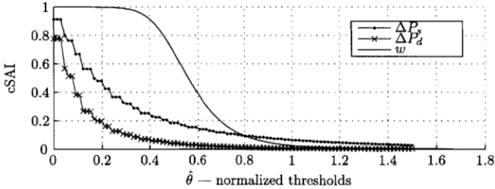
Figure 3-6 plots cSAI as a function of 3 abnormality criteria. Notice that each criterion flags only a small fraction of beats, and the slope of the curves are not steep but also nonzero

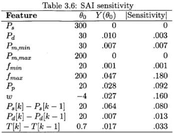
at 0 = 1. Table 3.6 lists the sensitivity of every parameter. The results indicate that our

study population had no waveform with P, > 300mmHg or Pm > 200mmHg.

U-1 0.6 0.4 0.2 0 -

...

I.

Figure 3-6: Perturbations to abnormality criteria. cSAI as a function of 3 parameters perturbations is shown. Sensitivity is defined to be the slope of each curve at 0 1.

Table 3.6: SAI sensitivity

Feature 9o Y(Oo) ISensitivityl

PS 300 0 0 Pd 30 .010 .003 Pm,min 30 .007 .007 Pm,max 200 0 0

fmin

fmax

3.3.3 Cardiac output estimation error

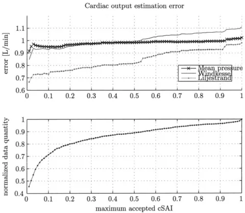
Figure 3-7 plots CO estimation error as a function of maximum accepted cSAI. Errors decrease for lower cSAI (cleaner waveform) values. For the Liljestrand algorithm, an error reduction of 30% is obtained. The mean pressure estimation algorithm is most robust to noise, as evidenced by its relatively flat line. This robustness is expected because of the simplicity and averaging nature of the mean pressure algorithm.

3.4

Discussion and conclusions

Evaluating the performance of the SAI algorithm is nontrivial, primarily because of a lack in the quantitative definition of an 'abnormal' beat of an ABP waveform. Consequently, there is no established gold standard to compare against. Furthermore, the definition of abnormality can be application dependent. For example, beat quality needs to be higher for CO estimation than for mean pressure tracking because more features derived from each beat are used for the former. From Figure 3-7, a maximum accepted cSAI level of 0.5 can

be routinely used for CO estimation purposes. At cSAI = 0.5, only 10% of the poorest

ABP data have been removed, CO estimation error has been substantially reduced, and the data quantity does not change very rapidly around this point.

From the sensitivity analysis, two abnormality criteria do nothing and have sensitivity of 0. Therefore, for our study population, they can be removed. Of the remaining criteria, pairwise correlation studies can be performed in the future to identify any redundant criteria. In conclusion, we have presented an algorithm that detects anomalies in the ABP wave-form. The SAI algorithm is in close agreement with a human expert (Table 3.5), is robust (Table 3.6), and has proven its effectiveness in its ability to select clean ABP waveforms to improve CO estimation.

Cardiac output estimation error

t 0.9

$0 0 .8 -. . . .. -. . . .-. -.- . .. . . . .

; - - Mean pres ure

0.7 -- - ra -0.6 0 0.1 0.2 0.3 0.4 0.5 0.6 0.7 0.8 0.9 1 0 .9 - -.-.-.-.- .- . -0.8 -- - ---0 .7 - -- -. --.-.- S0.6-0.5 0 S0.4 0 0.1 0.2 0.3 0.4 0.5 0.6 0.7 0.8 0.9 1

maximum accepted cSAI

Figure 3-7: CO estimation error as a function of maximum accepted cSAI. Bottom plot shows that the amount of data also decreases as we restrict ourselves to cleaner waveforms.

Chapter 4

Evaluation Methods

Evaluating the performance of cardiac output (CO) estimation requires obtaining the fol-lowing signals:

" A set of ABP waveforms as input for the CO estimators. In order to capture the

intra-beat waveform morphology, sampling rate of ABP needs to be sufficiently high (greater than 60Hz).

" A set of gold-standard CO measurements to compare with estimated CO. Each measurement must be available simultaneously to ABP waveform recordings. We will use thermodilution CO (TCO) measurements as gold-standard. It is well known that

TCO has errors itself [17]. Thus, by comparing estimated CO to TCO, our results

are limited by TCO's accuracy.

The signals will be processed by the following systems:

" A data extraction system to identify suitable ABP waveforms and TCO

measure-ments for analysis.

" A CO estimation system to accurately and efficiently implement each CO

estima-tion algorithm. Ideally, we obtain the 11 algorithms from the original creators and use their exact implementation. However, this is impractical in many ways. Hence, we peruse their publications and mimic their methods as closely as possible.

" A comparison system to output the error between each estimated CO and TCO.

This system may seem trivial, involving a simple subtraction. However, a major problem is that all CO estimates are given in relative units (Table 2.1). Therefore, we must establish suitable calibration methods before performing comparisons. We also design a scheme comparing percentage changes in estimated CO and TCO. This scheme does not require calibration.

" An error analysis system to report the performance of CO estimates across the

entire study population. We also explore the physiologic conditions in which CO estimators are likely to fail. Using these analyses, our goals are (1) to determine whether CO estimates are reliable enough for clinical use, and (2) to investigate the possibility of improving CO estimates.

Figure 4-1 presents a high-level flow chart showing the connectivity between the signals and systems outlined above. This chapter discusses each component in detail.

4.2

4.1 -ABP- Cardiac output -estimated CO 4.3 4.4

Clinical Data extraction estimation Comparison -error-* Error analysis

database

gold-standard C

Figure 4-1: A system for evaluating CO estimation performance.

4.1

Data extraction

Relevant source code: wavex.m, trendex.m 1

As described in Chapter 1, the clinical database we use is MIMIC II, which contains phys-iologic waveform data from over 3500 ICU patients hospitalized at Beth Israel Deaconess Medical Center, Boston, USA. From this database, we identified 120 patients with simul-taneously available ABP waveforms and TCO measurements. The ABP waveforms are measured radially and stored as 8-bit quantized data with a temporal resolution of 125Hz.

TCO is measured intermittently with a temporal resolution of 1 minute.

4.2

Implementation of CO estimators

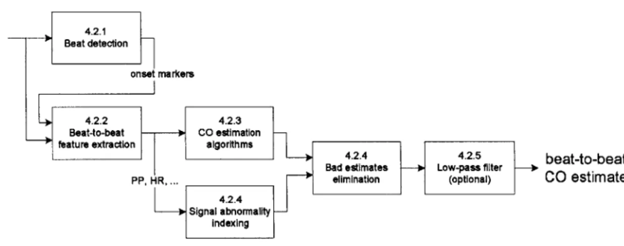
With appropriate ABP waveforms extracted, we are now ready to make CO estimates. Figure 4-2 presents the flow chart showing the transformation of ABP into beat-by-beat

CO. The first step is to detect beats in the ABP waveform. For each beat, various features

such as instantaneous heart rate, systolic blood pressure, and pulse pressure are extracted. Given the features, the CO algorithms output CO estimates. The signal abnormality indexer identifies abnormal beats and eliminates them. Finally, we apply a low-pass filter and eliminate fluctuations in CO estimates caused by beat-to-beat variations. The rest of this section discusses each major block of the CO estimation system in detail.

ABP 4.2.1

ABP >Beat detection

onsr markers

4.2.2 4.2.3

Beat-to-beat - - CO estimation

1feature extraction _algorithms

"424..5b

a-o e t

4.2.44.2.sbeat-to-beat

Bad estimates -- Low-pass filter -i

PIP, HR, .. elimination (optional) CO estimate

4.2.4 Signal

abnormality-Indexing

Figure 4-2: Data flow diagram for CO estimation.

4.2.1 ABP beat detection

Relevant source code: wabp.m

The beat detection system segments the ABP waveform into individual beats. The process

is essential in extracting ABP features. We adopt an algorithm designed by Zong et al. [22] that robustly detects the onset of each beat in the ABP waveform. The basis of Zong's onset detection algorithm is the slope sum function (SSF), which amplifies the rising part of each beat (Figure 4-3). More details can be found in their paper.

4-3: The slope sum function (SSF). It aids in onset detection. Figure adapted from

4.2.2 ABP feature extraction

Relevant source code: abpfeature .m

After segmenting the ABP waveform into individual beats, we extract useful features from each beat. The complete set of extracted features is listed in Table 4.1.

Table 4.1: ABP features

Feature Description Units

P Systolic blood pressure mmHg

Pd Diastolic blood pressure mmHg

Pp Pulse pressure (P, - Pd) mmHg

Pm Mean arterial pressure mmHg

As pressure area during systole (2 methods) mmHg-sec

w mean of negative slopes (for noise detection) mmHg/sec

T Duration of each beat sec

TS Duration of systole (2 methods) see

Td Duration of diastole (T - T,) sec

Figure 4-4 shows the identification of P,, Pd, and Pp. P, is the local maximum within

a time window following each onset. Likewise, Pd is the local minimum within a window

before each onset. P, is the difference between P, and Pd. Pm is the average of all pressure samples between adjacent onsets. T is the time difference between adjacent onsets. Noise level is defined as the average of all negative slopes in each beat.

As described in Chapter 2, many CO estimators require the detection of end-of-systole. End-of-systole's defining feature in the aortic pressure waveform is the dicrotic notch, mark-ing the time in which the aortic valve closes (Figure 4-5). Unfortunately, wave reflections and high frequency signal attenuation in the radial arteries completely mask the dicrotic notch. However, publications often mistakenly associate the second peak of each beat as the dicrotic notch. The second peak is not the dicrotic notch but a reflected wave.

This nontriviality in end-of-systole detection lead us to employ two techniques to ap-proximate end-of-systole, the RR method and the "first zero slope" (FZS) method. The

ABPI \J

-- JJI

S~~~~j

...

~

,

1n

./

11[

\__

.

...

It

...

Figure [22].

90 S80 70- S60-50 -0.4 -0.2 0 0.2 0.4 0.6 time [seconds]

Figure 4-4: Ps, Pd, and P, detection. The light dot marks the onset. The darker dots are P, and Pd. The line segment marks P,. The shaded areas are the two search windows for P, and Pd.

RR method uses a result from electrocardiography. QT-interval duration is approximated as 0.3/RR interval [1], where RR-interval is measured in seconds. Intuitively, the QT frac-tion becomes smaller as the durafrac-tion of a cardiac cycle lengthens. We approximate that the RR-interval equals the beat period. The QT-interval is the duration from electrical depolarization to repolarization of the ventricles. Therefore, for a normal healthy heart, we approximate the QT-interval and systolic ABP duration to be very similar. From Figure

4-5, these approximations are reasonable. Hence, T, = 0.3x/T. For the FZS method, we find

the first time following P, that the slope of ABP becomes 0. Preliminary testing showed that while the 2 methods may indicate significantly different end-of-systole times (Figure 4-6), both offered very similar results in terms of CO estimation performance.

The main purpose for end-of-systole detection is in calculating the area under ABP during systole of each beat. Figure 4-6 shows end-of-systole and systolic area.

As = f(P(t) - Pd)dt

T,

4.2.3 CO estimator implementation

Relevant source code: estO<num>_<title>.m

The first 9 CO estimators in Table 2.1 take features of the ABP waveform as input. Simple arithmetic operations are applied to produce beat-to-beat CO estimates. The last 2 esti-mators use beat-to-beat features and the raw ABP waveform. Differential equations are used to produce a flow waveform. Then, we integrate the flow waveform over the systolic duration to produce CO estimates.

4.2.4 Signal quality and bad beats elimination

Relevant source code: jSQI.m, estimateCO.m

Quality of the ABP waveform is essential in determining the performance of CO estimators. Noisy, artifactual, damped, and irregular (not sinus rhythm) ABP waveforms may easily lead to bizarre CO estimates. Figures 3-1, 3-4, 3-2, 3-3 from Chapter 3 show examples of ABP waveforms from MIMIC II in which CO estimates are likely to fail. In Chapter 3, we presented the SAI algorithm to flag abnormal beats in the ABP waveform. Flagged beats