HAL Id: tel-01263903
https://tel.archives-ouvertes.fr/tel-01263903
Submitted on 29 Jan 2016HAL is a multi-disciplinary open access archive for the deposit and dissemination of sci-entific research documents, whether they are pub-lished or not. The documents may come from teaching and research institutions in France or abroad, or from public or private research centers.
L’archive ouverte pluridisciplinaire HAL, est destinée au dépôt et à la diffusion de documents scientifiques de niveau recherche, publiés ou non, émanant des établissements d’enseignement et de recherche français ou étrangers, des laboratoires publics ou privés.
Developement of microscopy system for time-resolved
fluorescence detection of gadolinium/terbium hybrid
macromolecular complexes for bimodal imaging of
atherothrombosis
Trong Nghia Nguyen
To cite this version:
Trong Nghia Nguyen. Developement of microscopy system for time-resolved fluorescence detection of gadolinium/terbium hybrid macromolecular complexes for bimodal imaging of atherothrombosis. Physics [physics]. Université Paris-Nord - Paris XIII, 2014. English. �NNT : 2014PA132005�. �tel-01263903�
UNIVERSITÉ PARIS 13 - INSTITUT GALILÉE
LABORATOIRE DE PHYSIQUE DES LASERS-CNRS UMR7538
LABORATOIRE DE RECHERCHES VASCULAIRES TRANSLATIONNELLES–INSERM U1148
N° attribué par la bibliothèque
THÈSE
pour obtenir le grade de
DOCTEUR DE L’UNIVERSITÉ PARIS 13
Discipline : Physique
présentée et soutenue publiquement
par
NGUYỄN TRỌNG NGHĨA
Soutenue le 23 juin 2014
Développement d'un système de microscopie pour la
détection en temps résolu de la fluorescence de complexes
macromoléculaires mixtes Gadolinium/Terbium destinés à
l'imagerie bimodale de l'athérothrombose
Directeur de thèse : Jean-Michel Tualle
JURY
Mme Nathalie WESTBROOK Présidente Mme Florence GAZEAU Rapporteur Mme Hong Nhung TRAN Rapporteur M. Phalla OU Examinateur
M. Frédéric CHAUBET Co directeur de thèse M. Eric TINET Co directeur de thèse M. Jean-Michel TUALLE Directeur de thèse
This work was supported by the CNRS
(Centre National de la Recherche Scientifique)
through the contract number 254445
from march 2011 to february 2014
ACKNOWLEDGEMENTS
I would like to thank my supervisors Dr. Jean Michel Tualle, Prof. Frédéric Chaubet, Dr. Éric Tinet who have encouraged me throughout the course of this thesis and gave me valuable advices. I have gained important experience while working with them.
I would like to thank Dr. Anne Beilvert, Dr. Murielle Maire in the group Cardiovascular Bioengineering of Laboratory for Vascular Translational Science (LVTS) who have synthesized the agents needed for my experiments. In the same laboratory Graciela Pavon-Djavid and Liliane Louedec were very kind with me too when they helped me preparing the samples from the rats arteries.
I would like to thank my colleagues who are researchers in the departments of the Bichat Claude Bernard hospital: “Service Anatomie et Cytologie Pathologiques” and “Service de Radiologie et Imagerie Médicale”. They helped me a lot when I tried the in vitro and in
vivo experiments
I would like to thank my colleagues in the Laboratoire de Physique des Lasers (LPL) where I worked most of the time, in particular the secretaries, mechanics and optics technicians for their assistance.
Finally, I would like to thank the support and encouragement of my friends and my family, in particular my father, my mother and my wife.
Outline
INTRODUCTION --- 1
1-ATHEROSCLEROSIS, IMAGING AND CONTRAST AGENTS --- 3
1.1 Evolution of atherosclerosis --- 3
1.2 Platelets and atherothrombosis --- 4
1.3 Magnetic resonance imaging --- 5
1.3.1 Larmor frequency - Excitation --- 6
1.3.2 Relaxation --- 7
1.3.3 Imaging --- 7
1.4 MRI contrast agent --- 9
1.4.1 T2 contrast agent--- 9
1.4.2 T1 contrast agent --- 10
1.4.3 Bimodal MRI/optical contrast agents --- 10
1.5 Optical properties of terbium (Tb3+) and europium (Eu3+) ions --- 11
1.5.1 Absorption spectra --- 11
1.5.2 Emission spectra --- 13
1.5.3 Fluorescent lifetime --- 15
2-MICROSCOPE SYSTEM SETUP FOR TIME-GATED FLUORESCENCE --- 19
2.1 The microscope --- 19
2.2 The laser --- 20
2.3 The filters --- 22
2.4 The chopper --- 24
2.5 The EMCCD camera --- 24
Frame Transfer Mode --- 25
Non-Frame Transfer Mode --- 25
2.6 The shutter --- 26
2.7 The spectrometer --- 26
2.8 Electrical synchronization --- 26
2.10 “Mosaic” imaging --- 29
2.11 System background noise --- 30
2.12 Conclusion --- 31
3-THE EMCCD CAMERA --- 33
3.1 CCD camera --- 33
3.1.1 The transfer of charges --- 33
3.1.2 The CCD cameras architectures --- 34
3.2 Quantification of the signal provided by our camera --- 36
3.2.1 Theory --- 36
3.2.2 The function F0
( )
k and exponential constant g --- 393.2.3 Numerical method to estimate average number of photoelectrons λ at input -- 40
3.2.4 An example --- 42
3.3 Use of the Camera for Long Decay Fluorescent Measurement --- 49
3.3.1 Effect of vertical shift speed on the streaking of image --- 51
3.3.2 Application of vertical shift for lifetime measurement --- 57
3.4. Conclusion --- 61
4-P717-TB EXPERIMENTAL RESULTS --- 63
4.1 Synthesis of the fluorescent molecule --- 63
4.1.1 Synthesis of P717-Tb --- 63
4.1.2 Synthesis of P717-Tb-F --- 64
4.2 Optical properties of P717-Tb in solution --- 66
4.2.1 Spectrum --- 66
4.2.2 Fluorescent lifetime --- 67
4.2.3 Absorption cross-section --- 68
4.3 Fluorescent images of P717-Tb/PBS in healthy artery --- 71
4.3.1 Preparation of the samples --- 71
4.3.2 Fluorescent images --- 72
4.4 Conclusion --- 76
5-EXPERIMENTAL RESULTS ON ATHEROSCLEROTIC RAT ARTERIES -- 77
5.1 Animal model --- 77
5.2 Preparation of contrast agent mixtures --- 77
5.4 Preparation of the rat’s arteries --- 78 5.5 Results --- 79
CONCLUSION--- 83
APPENDIX A --- 85
APPENDIX B --- 89
REFERENCES --- 95
1
Introduction
According to the American Heart Association, atherosclerosis “is a type of arteriosclerosis. The name comes from the Greek words athero (meaning gruel or paste) and sclerosis (hardness). It is the term for the process of fatty substances, cholesterol, cellular waste products, calcium and fibrin (a clotting material in the blood) building up in the inner lining of an artery. The buildup that results is called plaque” [1].
The development of atherosclerosis is usually a long process and its causes are not clear. Many scientists think atherosclerosis starts from the damages of the innermost layer of the artery. The reasons of those damages could be
+ High amounts of certain fats and cholesterol in the blood + High blood pressure
The biggest risk of atherosclerosis is a heart attack or a stroke that cause irreversible damages to the brain or the heart, possibly a sudden death. Because the development of atherosclerosis is over decades, an early detection of disease is very important for the treatment.
Since the pathology is deeply located in utmost important organs, a direct invasive observation would be extremely difficult and would be extremely dangerous. Moreover, the affected regions may be diverse and of varying sizes. Therefore, a good diagnostic method should both be non-invasive and independent on the pathology’s locations.
Blood cells are implied from the very beginning of the pathological process. In particular platelets play a pivotal role in cardiovascular diseases and there is a great interest in diagnostic approaches enabling activated platelet molecular imaging i.e. thrombotic pathological situation because platelets constitutes the main cell part of the thrombus.
Magnetic resonance imaging (MRI) is a method which can image the whole body. It could be a good technique to diagnose atherosclerosis, but its spatial resolution isn’t yet very good and the natural contrast between atheroma and its surrounding tissues may be poor. One can notice that if someday MRI achieves a one-cell or a sub-cellular resolution, the volume of data to acquire and to process would be really big! Moreover, ultimate MRI resolution will probably be limited for routine diagnosis by biological safety norms (maximum fields intensity, time derivative of fields, duration of exposure). For all these reasons, in MRI technique, a contrast agent is often used – and will be in the future - to enhance the contrast of the images or to label specific tissues or lesions we may want to localize in the body. It is therefore evident that an agent providing a high contrast while being very specific to the arteries lesions, at early stages if possible, with a low toxicity and side effects (intrinsically innocuous and/or efficient at low concentrations) is extremely desirable.
Since 2003, the Laboratory for Vascular Translational Science (formerly Laboratory for Polymer Bioenginneering) has developed with the company Guerbet Laboratories the use of a macromolecular MRI contrast agents (P717) including a gadolinium-based complex with a ligand (DOTA). The magnetic contrast can be appropriate, but the limitation due to the low spatial resolution of the MRI technique [2], [3], [4], [5] still persists and does not allow research on the cellular level, even on extracted samples.
2
The idea is to slightly modify the contrast agent to allow the study of its interactions with the tissues using another imaging modality which sensitivity and resolution would be complementary to that of MRI. If we substitute terbium ions to the gadolinium ones, the chemical properties of the agent isn’t noticeably modified. However, the terbium ions are fluorescent, and the spatial resolution of an optical system can be well below one micrometer. Excitation wavelength is in the ultra-violet range. Fluorescence efficiency is very low, well below tissue autofluorescence, but since it has a very long emission time, a time-gated detection is feasible. UV excitation and low efficiency fluorescence is not possible in vivo as a routine diagnostic method. However, we can obtain on histological slices valuable information about the contrast agent’s interaction with the arteries wall and the atherosclerotic pathologies.
We will start from the macromolecular precursor of P717, Gd and Tb complexes to obtain Tb and Gd complexes. Then these complexes would be endowed with biospecificity by coupling them with a ligand exhibiting a strong affinity for activated platelets. By mixing both biospecific contrast agents it should be possible to localize by MRI the pathological areas in vivo (rat model) and after sacrifice of the animals to visualize the thrombus at cellular scale with delayed fluorescence imaging of histological slices.
Fluorescence microscopy is widely developped for the examination of slices of tissues with the use of organic fluorophores for example linked to antibodies for the identification of tissues areas, cells or macromolecular biological structures. Beyond this use, organic fluorophores have numerous drawbacks when considering quantification and specificity of the signal. Thus there is a strong need of a system allowing to localize and efficiently quantify even very low amounts of contrast agent in situations where they are able to specifically bind to pertinent ligands of atherothrombosis, in our case: activated platelets. Fluorescence molecular imaging is the first challenge of this project. The second one is to get both MR and optical images from the same contrast agent, knowing that water molecules needed for the MR contrast are powerful quenchers of lanthanide fluorescence.
3
Chapter 1
Atherosclerosis, imaging
and contrast agents
1.1 Evolution of atherosclerosis
It has long been thought that atherosclerosis was similar to a clogged pipe, where the pipe is a passive victim of a buildup of fatty materials and limescale, except that maybe it can show a little surface corrosion which acts as an anchor point. The development of atherosclerosis is presented in the figure 1.1 [6], [7], [8].
However, in fact, it is an extremely complex and still not fully understood pathology where the artery walls play an active role. All children older than age 10 have primary anatomic lesions. Sometimes, it even starts as young as one year old. No one is immune; the early stage seems to be independent on the geographic origin, the sex, the environment. The pathology initially evolves very slowly and during the first two or three decades, it is completely silent. Nevertheless, we know for sure that after this slow asymptomatic evolution, the atheroma evolves faster later and this speed depends heavily on some environmental factors like stress, food, exercise.
The pathology starts with repeated injury to the wall of arteries. A higher than normal blood pressure and shear stress in the blood flow are probably important factors here. In fact, for the animal models, like rabbits, used to study atherosclerosis, the pathology is initiated by scratching the inner wall of a coronary artery, and then by feeding the animals with a very fatty diet. The injury leads to an answer by the immune system and macrophages penetrate the artery wall. For some reason, they stay blocked here. When the macrophages die, their materials, for example their cholesterol-rich membranes stay in place in the middle of artery wall. This enhances the inflammation and more macrophages are attracted here. This process is the core of the first silent phase. When enough lipids are accumulated in the artery’s wall, fibrosis and calcification appear. The artery is partially blocked. Its wall becomes rigid and can rupture.
Of course, the sooner we can detect the pathology, the easier and least difficult is its mitigation. Imaging plays a key role here, and the two main methods of clinical imaging are X-ray tomography and Magnetic Resonance Imaging.
4
Figure 1.1: The development of atherosclerosis [6].
1.2 Platelets and atherothrombosis
When the atherosclerotic vessel is ruptured, thrombogenic substances are exposed and platelets contribute to the pathophysiologic process via adhesion, activation and aggregation stages [9]. At a cellular level, phenotypical and morphological modifications of vascular cells are observed early in atherosclerosis [10] and platelets represent a major link between inflammation, thrombosis and atherogenesis [11], [12]. Beside, activated vascular cells overexpress lectins, such as E-selectin, L-selectin and P-selectin, and proteoglycans on their surface. These are glycoconjugates which carbohydrate moieties play a critical role such as cell-cell interactions, cell growth, lymphocytes trafficking, thrombosis, inflammation, host defense or cancer metastasis [13], [14], [15]. P-selectin, overexpressed on activated platelets,
5
is recognized by a natural ligand PSGL-1 (P-selectin glycoprotein ligand-1) expressed by lymphocytes via the tetrasaccharide sialyl LewisX [17]. Structural features of sialyl LewisX are essential for the recognition of PSGL-1: the hydroxyls of L-fucosyl and D-galactosyl, carboxylic group of sialic acid [16], and sulfated tyrosines in the protein backbone [18].
Fucoidan, heparin and dextran sulfate are sulfated polysaccharides which bind to P-selectin [19], [20] mimicking the interaction with PSGL-1. Low molecular weight fucoidan was formerly demonstrated to be of potential interest for revascularization in cardiovascular diseases [21], [22] and found as the most efficient glycosidic ligand of P-selectin in purified system and in human whole blood experiments [19]. The large amount of P-selectin in platelet-rich thrombi formed after atherosclerotic plaque rupture or erosion makes it a good target for fucoidan.
In this context, P-selectin appears as a good candidate target for the diagnosis of atherosclerosis and a contrast agent able to bind to P-selectin, i.e. vectorized by fucoidan to activated platelets, would efficiently enhance the detection of early thrombus formation.
1.3 Magnetic resonance imaging
MRI is one of the imaging modalities used in this work. One can use MRI like X-ray imaging to measure the artery wall thickness and to assess the blood flow. But one can also use a magnetic contrast agent. The sensitivity to the contrast agent is proportional to the number of magnetic atoms, not the volume of the observed region. If the agent is very specific of a pathology, it will make a bright localized source regardless of its size. This is exactly what we want to do here: to have a contrast agent which binds to the early stages of atheroma that we can detect in a non-invasive manner by MRI.
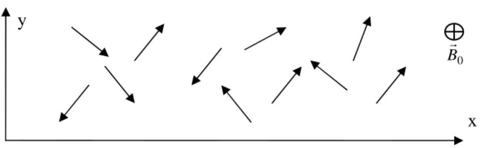
The magnetic properties of a nucleus are characterized by its spin. Each nucleus acts like a tiny magnet and therefore can be represented by a vector (figure 1.2). Normally, the direction of the spin vector is random. As a consequence, in a large collection of nuclei, the sum of all the spin vectors – called net magnetization - is zero.
Figure 1.2: The spin of a nucleus is like a tiny magnet
When an external magnetic field B0 r
is applied, their spin vectors will align in a given direction which is determined by the laws of quantum physics.
6
Figure 1.3: Spin vectors align in an external magnetic field
The hydrogen nucleus (namely a proton) is the most frequently imaged nucleus in MRI because it is present in biological tissues in great abundance and it gives a strong signal. The hydrogen nucleus can be in one of the two states (figure 1.3):
- The spin vector aligns with the external field. That corresponds to the lower energy level.
- The spin vector aligns against the external field. That corresponds to the higher energy level.
In fact, the spin vector is not perfectly parallel to the vector of the external magnetic fieldB0
r
, it precesses about the axis of the external field (figure 1.4)
Figure 1.4: The precession of the spin vector
1.3.1 Larmor frequency - Excitation
The precession frequency – Larmor frequency – is: 0 0
γ
Bω
= (1.1)Each isotope has its own Larmor frequency.
The magnetic vector of the spinning protons includes two orthogonal vector components: a longitudinal or Z component - Mz, and a transverse component, lying on the XY plane – Mxy. In the external magnetic field, there are more spins aligned with the field than spins aligned against the field. Therefore, the net magnetization has a longitudinal
B0 z y x Mz Mxy y x Mz Mxy z B0
7 component aligned with B0
r
. As spins do not rotate in phase, the transverse component of the net magnetization is null (figure 1.5).
Figure 1.5: The random phases of the transverse component of spin vectors gives a null average magnetization
When hydrogen nuclei are excited by a radio frequency (RF) signal at the Larmor frequency, some nuclei can absorb RF energy and jump to a higher energy level – or change the direction of their spin vector to align with the external field. Two phenomena occur simultaneously:
First, all vector spins precess in phase => Mxy ≠ 0
Secondly, the number of nuclei in the higher energy state increases. Mz decreases. If Mz = 0, the excited pulse is called a 900 RF pulse because this pulse cause the net magnetization to flip 900 relative to the xy plane. If direction Mz changes to the opposite direction, the excited pulse is called a 1800 RF pulse.
1.3.2 Relaxation
When RF pulse terminates, the relaxation process begins. The relaxation combines two mechanisms:
On one hand, a nucleus emits a RF signal when returning to the lower energy level. Mz recovers its initial state. This is characterized by a longitudinal magnetization recovery time constant T1. In general, T1 values are longer at higher field strengths.
On the other hand, the vector spins get out of phase due to spin-spin interactions, Mxy decreases to null. This is characterized by a transverse magnetization decay time constant T2.
T1 is around one second while T2 is a few tens of milliseconds. The values of T1 and T2
are widely different in different tissues. Imaging uses this difference.
1.3.3 Imaging
Now, how does the MRI work?
To get the 3D MRI, one must “cut” the body in several 2D slices
The spatial encoding
We know that only the RF frequency which coincides with the Larmor frequency has some effects on the nucleus. So the system applies a static magnetic field inside the imaging region with a known gradient. Different spatial slices correspond to different precession frequencies. y x 0 B r
8
Then, we apply pulses of gradients of the magnetic field (gradient echo) or pulses of the RF excitation (spin echo) to select a narrow region.
This process can be repeated when the spins approximately returned to their thermal equilibrium. The whole body is scanned this way.
There is a very large number of possible magnetic and RF pulses configurations, and different manufacturers optimize their hardware and software differently.
Contrast
Contrast is caused by the differences in the MR signal. It helps to distinguish the different tissues. Contrast depends on tissue properties, the T1, T2 relaxation times and the proton density of the tissue, and on machine properties, the sequence of pulses parameters.
For example, we consider a spin-echo sequence, which is a common procedure. This sequence uses a 90o RF pulse followed by an 180o RF pulse. Spin-echo sequence has two main parameters:
• Echo Time (TE) is the time between the 90° RF pulse and MR signal sampling (the start of MR signal acquisition). The 180° RF pulse is applied at time TE/2.
• Repetition Time (TR) is the time between 90° RF pulses.
Table 1.1: Three weighted modes of a spin-echo sequence.
TE
Long Short
TR
Long
T2 – weighted
The contrast is caused mostly by the different T2 values
(tissue with a longer T2 is brighter)
Proton density – weighted
The contrast is caused mostly by the different of the proton density.
Short
No signal T1 – weighted
The contrast is caused mostly by the different T1 values (tissue with a shorter T1 is
brighter)
In the clinical practice, the values chosen for TR and TE followed these rules [23]:
• TE is always shorter than TR
• A short TR = value approximately equal to the average T1 value, usually lower than 500 ms
• A long TR = 3 times the short TR, usually greater than 1500 ms
• A short TE is usually lower than 30 ms
• A long TE = 3 times the short TE, usually greater than 90 ms
As an example, the figure 1.6 present a transversal image recorded from a rat we used for our experiments (see Chapter 5 for experimental conditions).
9
Figure 1.6: transversal image of a rat abdomen. The parameters are mentioned on each side of the image: Magnetic field = 7 T, slice width = 0.9 mm, Matrix of the image 256x256, TR =
1742.9 ms, TE = 9 ms etc…
1.4 MRI contrast agent
MRI contrast agents are by definition designed to enhance the contrast. Their main effect is the shortening of the relaxation times T1 and T2 of the hydrogen nuclei of water molecules which surrounds them. The capability of shortening the T1 and T2 relaxation times is described by the term "relaxivity". The relaxivity is the increase of longitudinal or transversal relaxation rate, 1/T1 or 1/T2 respectively, and is denoted by r1 and r2. The relaxivity of the contrast agent is the increase of the relaxation rate due to the contrast agent per unit of concentration of the agent. In presence of a contrast agent, the observed relaxivity (1/Tx, with x=1 or 2) is the sum of the intrinsic relaxivity of the examined aera in absence of contrast agent (1/Tx0) and that of the contrast agent (1/Txa). The slope of the curve obtained by plotting 1/Tx vs the concentration of agent gives the relaxivity rx of the contrast agent [24], [25]. In general, r1 decreases when the magnetic field becomes stronger, whereas r2 tends to remain constant or even can increase somewhat [25].
The ratio between the relaxation rates r2 and r1 determines whether a contrast agent is
suitable for the enhancement of T1-weighted or T2-weighted imaging.
1.4.1 T2 contrast agent
The most effective T2 contrast agent are nanoparticles of magnetite (Fe3O4) or maghemite (γ-Fe2O3). These are also called superparamagnetic contrast agents [26], [27]. With a diameter ranging from 4 nm to 50 nm, the superparamagnetic agents contain thousands paramagnetic Fe ions (Fe2+ and/or Fe3+). Therefore it has a large magnetic moment in an external magnetic field. As a result, superparamagnetic agents introduce strong local field gradients, which accelerates the dephasing of the surrounding water protons [28], i.e induces a shortening of T2 and an increase of r2.
Depending on their size, their crystalline structure, and their coating, superparamagnetic agents are called: superparamagnetic iron oxide particles (SPIO),
10
small superparamagnetic iron oxide particles (USPIO), very small superparamagnetic iron oxide particles (VSOP), monocrystalline iron oxide particles (MION) and cross-linked iron oxide particles (CLIO) [29], [30], [31], [32], [33].
1.4.2 T1 contrast agent
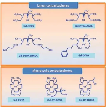
Gadolinium ion (Gd3+) is the most common T1 contrast agent used in the clinic environment because it has a high paramagnetic moment. However the free ion Gd3+ is toxic for living tissue like most free ion metals are. Therefore, gadolinium ions need to coordinate with a suitable ligand to form a nontoxic complex. The figure 1.7 [34] present some of the most common commercial gadolinium-based contrast agents: DTPA (Magnevist), Gd-DOTA (Dotarem), and Gd-HP-DO3A (Prohance).
Figure 1.7: Some of the most widespread gadolinium based MR contrast agents
The relaxation mechanism of T1 contrast agent is described by Solomon-Bloembergen-Morgen (SBM) theory [35], [36], [37]. The relaxation is mainly due to the interaction between Gd3+ and water molecules, which directly coordinate with Gd3+ ions. This interaction is characterized by the exchange correlation time τm. In the complex, Gd3+ usually has one directed coordination with a water molecule. The rotation of a complex is also important: because the rotation frequency of Gd complexes is fast compared to the Larmor frequency, the slowing down of complexes closer to the Larmor frequency improves the relaxation. The effect of the complex rotation is characterized by the rotational correlation time τr. One way to improve the relaxation of Gd complexes is to link many Gd chelates on a macromolecule. The consequences are both the increase of the rotational correlation time and that of the local concentration of Gd3+ ions.
1.4.3 Bimodal MRI/optical contrast agents
In MRI, the use of contrast agents enables image enhancements and therefore opens the way towards more reliable diagnosis. Nevertheless, the best MRI resolution is a few dozen micrometers [2] and such a high resolution requires a long acquisition time. This limitation is not suitable with the study of the distribution of the MRI agents in small volumes like in a single cell or even into the layers of a small artery wall. Yet, if we want to study why a given agent exhibits some affinity for a pathologic tissue, or if we want to modify the agent in order to increase this affinity, we need a very high resolution imaging method. The resolution of
11
MRI is far worse than the resolution of optical microscopy. Of course, optics is a good imaging method!
To overcome this obstacle, many efforts were done to synthesize fluorescent MRI agents. Many different fluorophores can be linked with MRI agents [38], [39]. However, biological tissues are naturally fluorescent too. Of course, biological tissues are not intensely fluorescent, but modified MRI agents aren’t very bright either. To make things worse, emission wavelengths of the main fluorophores used for agents fall in the emission regions of the tissues autofluorescence, making it sometimes difficult to interpret the images. Hence we need to develop more sophisticated markers, for example fluorophores capable of emitting in the near infrared where the fluorescence of the tissues is absent [40]. Another way to solve this issue is to use fluorescent emitters which decay very slowly, a lot longer than the time constant of the autofluorescence decay. Lanthanide complexes, particularly europium and terbium, have been used for forty years in analytical biochemistry [41], [42] with several advantages compared to purely organic fluorophores [43], [44]: very long luminescence decay (some hundred microseconds to some millisecond), better photostability, narrow emission lines and large Stokes shift. These compounds can therefore achieve fluorescence optical imaging with a time-resolved emission in the visible (green light for terbium and red light for europium) easily discriminated from the background noise.
Gadolinium, europium and terbium are lanthanides and have the same physicochemical and biological properties. An MRI contrast agent which would have some of its Gd3+ ions replaced by Eu3+ or Tb3+ ions would make possible a time-gated fluorescence microscopy in the visible wavelengths. Because of the similarity between the lanthanides, and because the metallic ions are shielded from the biological activity, the modified optically active agent can’t be noticeably different chemically from the pure MR one. Therefore, any useful information collected using this modified agent remains pertinent for the original agent.
1.5 Optical properties of terbium (Tb3+) and europium (Eu3+) ions
1.5.1 Absorption spectra
The absorption spectra of free ions Gd3+, Eu3+ and Tb3+ in aqueous solution are presented in the figure 1.8, 1.9, 1.10 [45, p. 179]. The vertical axis represents the molar absorptivity ε (also called molar absorption coefficient or molar extinction coefficient) of the solution. The molar absorptivity is defined by the formula [46, p.33]
I I cd 0 log 1 = ε [L.mol-1cm-1] (1.1)
where I0 is the intensity of the incoming light, I is the intensity of the outgoing light, c is the concentration in moles per liter, d is the path length in centimeters. The relation between the
molar absorptivity and the absorption cross-section σ is [46, p.33]
ε
σ
21 10 82 . 3 × − = [cm2] (1.2)The top horizontal axis represents the wavelength in nanometers. The bottom horizontal axis represents the wave number in cm-1.
12
Figure 1.8: The absorption spectrum of Gd3+ in an aqueous solution
Figure 1.9: The absorption spectrum of Eu3+ in an aqueous solution
13
It is clear that Gd3+ only absorbs in the middle UV light. This is not convenient because exciting it requires a quartz optical system and a powerful source in a region where few lasers are available. On the contrary, Eu3+ and Tb3+ have some wide band absorption in the near UV region. They can be excited by a very compact light source like a LED or a laser diode.
It is worth to remark that the molar absorptivity of Eu3+ and Tb3+ is very much smaller than the one of the common fluorophores like Carbostyryl 7 (1.46 x 10⁴L.mol-1cm1- @ 350 nm), Coumarin 4 (2.10 x 10⁴L.mol-1cm1- @ 372 nm), DASPI (3.83 x 10⁴L.mol-1cm1- @ 372 nm) … [46]. As a result, the fluorescent intensity we can expect from Eu3+ and Tb3+ is very low. This is the main obstacle that we must overcome when designing applications with Eu3+ and Tb3+.
One straightforward way to increase the fluorescent intensity collected from Tb3+ and Eu3+ ions is to increase their local concentration. They can be added like dopants in a nano particle like yttrium vanadate [47], [48] or coated on the surfaces of SiO2 nano particles [49].
Fluorescence resonance energy transfer (FRET) is also used to increase the absorption of excitation light. The excitation light does not excite directly the lanthanide ions. It excites particles which have a large molar absorptivity, and then these particles transfer the excited energy to the nearby lanthanide ions [49], [50], [51], [52].
1.5.2 Emission spectra
Figure 1.11 shows the energy level diagram of lanthanide ions in aqueous solution. It is clear that the emission peak of Gd3+ is around 310 nm. Acquiring this wavelength require also quartz optical system and UV detector. Therefore, Gd3+ is really not suitable for fluorescent microscopy imaging, both from the absorption and emission points of view.
Eu3+ and Tb3+ have emission in the visible region as shown in the figure 1.12. This is adapted to a conventional microscope.
It should be noted that while the emission spectra of Tb3+ is almost not changed with different ligands, the relative intensity of peaks in the spectra of Eu3+ depends strongly on the ligands (figure 1.13 and [53]).
14
Figure 1.11: Dieke diagram of free lanthanide ions [54, p.8]
15
Figure 1.13: Normalized emission spectra of europium complexes [56]
1.5.3 Fluorescent lifetime
The table 1.2 shows the very long fluorescent lifetimes of Eu3+ and Tb3+ ions. They last approximately 10 milliseconds. In fact, fluorescent lifetimes of these ions in aqueous solution are much shorter. They last only about 0.45 milliseconds for Tb3+ and 0.13 milliseconds for Eu3+ [57], [58], [53], [59]. The interaction of Tb3+ and Eu3+ with water molecules is the one reason [57], [60], [58]. Therefore, the binding of Eu3+ and Tb3+ with a ligand is a good solution to eliminate this interaction.
The table 1.3 shows the fluorescent lifetime and quantum efficiency of Eu3+ and Tb3+ in H2O and D2O solutions. It is clear that Eu3+ and Tb3+ in complexes have longer fluorescent lifetimes and therefore a higher quantum yield. One can note that the data shows that the increase of the quantum yield usually is higher than the increase of the fluorescent lifetime.
16
Table 1.2: Calculated radiative lifetimes of excited states of lanthanide ions in an aqueous solution [54, p. 197]
Table 1.3: The fluorescent lifetimes and quantum yields of Eu3+ and Tb3+.
H2O D2O Ref. Fluorescent lifetime (ms) Quantum yield (%) Fluorescent lifetime (ms) Quantum yield (%) Eu3+ (aqueous) 0.13 0.9 1.65 11.2 [58] Eu3+ (aqueous) 0.10 2.27 [59] EuEDTA 0.26 2.05 Eu3+ (aqueous) 0.65 [55] Eu3+ (aqueous) 0.11 2.86 [53] EuDOTA 0.60 2.13 EuDPA 1.54 2.94 EuEDTA 0.34 2.10 EuDTPA 0.63 2.27 EuDTPA-cs124 0.62 16.7 2.42 65.2 [50] EuTTHA-cs124 1.19 42.3 1.79 63.6 EuDOTA-cs124 0.62 13.7 2.25 49.7 Tb3+ (aqueous) 0.48 3.4 2.39 16.7 [58] Tb3+ (aqueous) 0.43 3.3 [59] TbEDTA 0.41 3.20 Tb3+ (aqueous) 0.47 1.3 [57] Tb3+ (aqueous) 2.9 [55] TbDTPA-cs124 1.55 48.6 2.63 81.8 [50] TbTTHA-cs124 2.15 73.0 2.37 80.6 TbDOTA-cs124 1.54 43.6 2.61 74.9 Tb(DTPA-2pAS) 1.45 7.67 [61]
17
We can increase the signal to noise ratio (SNR) of Eu3+ and Tb3+ ions fluorescence in an organic medium by taking advantage of their long fluorescent lifetimes. Organic matter emits a strong autofluorescence under UV illumination. Its fluorescent lifetime is several nanoseconds. It is very short compared to the fluorescent lifetimes of Eu+3 and Tb3+. Therefore, if we acquire the Eu3+ and Tb3+ fluorescence emission after the decay of the tissue’s autofluorescence we can obtain a considerably increased SNR [38], [41], [62], [63], [64], [65] despite a lower total energy capture (we lose the fluorescence emitted at shorter times). This technique is named time-resolved or time-gated fluorescence. The principle of the time diagram for this technique is shown in the figure 1.12.
Figure 1.14: Principle of time-gated fluorescence
t t t excitation pulses autofluorescence (…) and Ln3+ fluorescence ( ___ ) acquired data trigger
19
Chapter 2
Microscope system setup
for time-gated fluorescence
We built a microscope system designed to acquire low intensity, long lifetime, fluorescence images of artery specimens labeled by the P717Tb complex. The time-gated technique is used to discard the strong “fast” autofluorescence which comes from organic samples under UV light.
This system is capable to measure the fluorescent spectrum of artery specimens excited by UV light.
For colorized samples, the system supports a color imaging acquisition.
2.1 The microscope
We must excite the samples fluorescence with UV light. Therefore, all the optical elements in the excitation path must transmit UV with a good efficiency and emit minimal parasitic fluorescence. Samples fluorescence is emitted in the visible region. It is mainly green. Ordinary microscope optics is suitable here. We also wish to be able to perform tissues identification, in order to determine where the fluorescent marker is fixed. An anatomo-pathologist must have a good quality color image for this identification. If the color and fluorescent image are acquired exactly by the same experimental setup, it is easier to make the correspondence between the two images. No software rescaling, translation, etc is necessary.
An inverted microscope perfectly corresponds to all these needs. Therefore, the microscope fluorescence system was built from an Axio Observer A1m inverted microscope. Above the sample’s platform, we are free to build the illumination system without constraints about shape and size. All the microscope functions are below the sample’s platform. Fluorescence is seen as ‘transmitted’ through the sample. We still need a filter to block UV propagation into the microscope system, somewhere after the sample (labeled F2 in the following, see figure 2.14). White light illumination, for the color image, comes from below and the color image is “reflected’ from the sample. The image path and camera is the same for fluorescence and color images.
This microscope has two output ports. Four objective lenses EC Epiplan whose magnifications are respectively: 10x, 20x, 50x and 100x.
20
2.2 The laser
The terbium ions require an excitation by UV light as described in the previous chapter. We have chosen a laser diode as a source for excitation because it possesses valuable properties: it’s compact, operates in continuous wave and pulsed modes, its output power can be easily adjusted and it can be synchronized with other parts of system.
We bought a Laser Stradus 375 made by Vortran Medical Technology, Inc. Some parameters of this laser are shown in the table 2.1:
Table 2.1: Specifications of the Vortran UV laser
Center wavelength (nm) 371
FWHM (nm) 2
Power output (mW, CW mode) 15
Spatial mode TEM00
Beam diameter (mm, 1/e2) ~ 1.3
Beam divergence (mrad) ~ 0.5
M2 < 1.25
Beam circularity > 90%
Polarization extinction ratio > 100:1 Power stability (over 24 hours) < 0.5%
Digital modulation 200 MHz
Digital rise time < 2ns
Analog modulation 500 kHz
Analog rise time < 0.7 µs
Operating temperature 10oC to 45oC
Figure 2.1: The UV laser head
We measured the emission spectrum of this laser on an EG&G 1461 digital triple grating spectrometer. It shows only one narrow peak at 371 nm (figure 2.2). This wavelength is suitable to excite terbium ions.
However, we encountered two problems.
The first one was easily solved: the laser emits some visible light at the wavelength we want to observe. Maybe it comes from some fluorescence from the laser’s materials; maybe it’s due to some emission between junctions in the laser. In any case, a good filter (labeled F1 in the following, see figure 2.14) centered on the emission wavelength should rule out this parasitic emission.
21
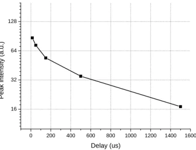
The second problem was a little more difficult to deal with: when the laser pulse is switched off, UV light at 371 nm is still emitted by the laser chip (figure 2.3). This light emission decays during some hundred microseconds. It decreases faster than an exponential decay function. This residual UV light is extremely weak compared to the ordinary UV laser emission, but it can cause autofluorescence in biological samples and on some of the glass optics in the microscope. Autofluorescence is a lot more intense than our desired signal and can overwhelm the signal from terbium ions. One mechanic chopper must be used to eliminate the residual light (see section 2.4)
330 340 350 360 370 380 390 400 410 420 0 300 600 900 1200 1500 1800 2100 2400 2700 3000 In te n s it y ( a .u ) Wavelength (nm)
Figure 2.2: The UV laser emission spectrum
0 200 400 600 800 1000 1200 1400 1600 16 32 64 128 P e a k i n te n s it y ( a .u .) Delay (us)
Figure 2.3: The residual UV light at 371 nm (in a logarithmic scale) .
The absorption of energy by the terbium ions is very low; moreover, the power of our UV laser is low too. Its maximum power in continuous mode is 15 mW. The specimens is only receive 5 mW due to losses on the filter F1 and the focus lens.
The laser beam diameter (FWHM) is approximate 0.76 mm, so the average intensity on a specimen is only 1W/cm2.
22
A single focusing lens is used to concentrate laser light on a specimen. The size of the laser spot on the specimen is adjusted by changing the distance between the lens and the specimen. That's the way we used to choose the adequate light intensity by defocusing.
(a) (b)
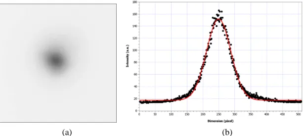
Figure 2.4: Image of the laser spot at the sample’s position
The figure 2.4a shows the image of a fluorescent spot of terbium in a solution when it was excited by the UV laser. This was also the real image of laser spot’s size. The chart in the figure 2.4b is the power distribution of the laser beam (vertical cut in figure 2.4a). We fit this data to a Gaussian function
(
)
− − + = 2 2 0 0 2 exp w x x A y yand the comparison gives us w = 38.0 ± 0.2 pixels. The FWHM diameter equals 89.3 pixels. By taking a standard image, we estimate that the distance between two pixels is equivalent the distance of 0.7 micrometer on the specimen. Therefore, the FWHM diameter of laser beam is approximate 62 micrometer. The average intensity on a specimen now is 182 W/cm2.
The field of view of the objective 20x is approximately 1 mm. Therefore, only one small part of specimen is excited. To get a full image of specimen, we need scan the laser spot on the specimen. The image area around each excited position is collected. Those data will be used to build by software the whole fluorescent image of the specimen.
2.3 The filters
The first single filter (F1) eliminates the parasitic visible light from the excitation laser. We purchased it from Horiba, code EM XF01 330WB60. The transmission spectrum of this filter is shown in the figure 2.5
The second single filter (F2) is the Semrock filter with has the code LP02-442RS-25. It is a broadband high-pass filter. This filter is placed after the microscope objective to block the UV laser light (317 nm) from propagating further into the microscope and possibly creating autofluorescence in it. This filter allows the transmission of the fluorescence emitted by the terbium ions in the visible region. The transmission spectrum of this filter is shown in the figure 2.6.
23
Figure 2.5: The transmission spectrum of the EM XF01 330WB60 filter
Figure 2.6: The transmission spectrum of the LP02-442RS-25 filter.
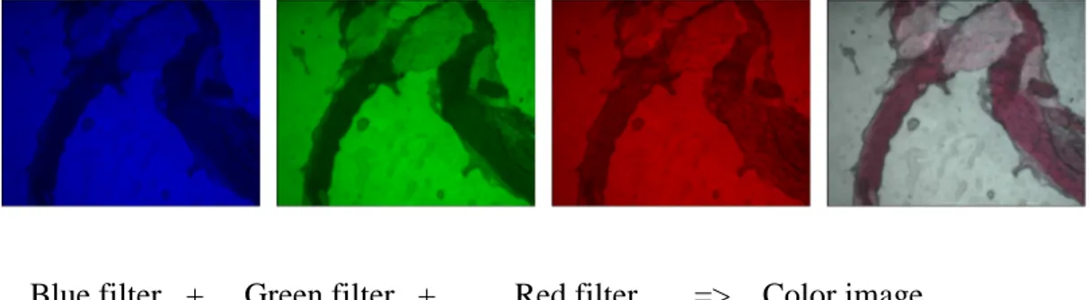
The filter set (FS) includes three optical cast plastic color filters from Edmund Optics. The colors transmitted by those filters are successively red, green and blue. We use them to synthesize a color image, as we’ll explain below. We place them between the white light halogen lamp of the microscope and specimens. The color of the illumination light is chosen by selecting one of those filters. For each color, the camera gives us a “gray scale” image. Then the three gray scale images, corresponding to the three primary colors of the RGB image, are assembled with the corresponding weights. The result is a real color image of specimens (see figure 2.7)
Blue filter + Green filter + Red filter => Color image
24
2.4 The chopper
The mechanic chopper was made by EG&G Instruments (model 651). eliminates the residual light of UV laser. Our working frequency is 80 Hz. The TTL timer signal is used as the master synchronizing pulse of the whole system.
2.5 The EMCCD camera
Since the power of the fluorescence signal of the metallic ions is low, we need a very good camera to get a correct signal to noise ratio. The camera we have chosen is an Andor iXon3 DU-897D. We estimated it could be sufficient to acquire the fluorescent image of artery specimens when they are labeled by our bimodal contrast agent. This camera has an up to 1000x electron multiplication gain and its sensor can be cooled down to -100oC to get a very low dark current noise. Therefore, it can acquire a very low intensity image. The camera module is fitted with an external trigger port to allow the camera to be synchronized with other parts of the system like the chopper and the UV laser diode. We give more details about the specifications of this camera in the table 2.2. The spectrum sensitivity of the camera covers completely the visible range with a high quantum efficiency. Its maximum sensitivity is obtained from 500 nm to 700 nm. That matches very well the emission spectrum of terbium ions (figure 2.8).
Table 2.2: Specifications of the Andor iXon3 DU-897D camera
Sensor CCD
back illuminated standard AR coated Blemish specification Grade 1 sensor (CCD97)
Active pixels 512 x 512
Pixel size (µm) 16 x 16
Image area (mm) 8.2 x 8.2 (100% fill factor) Cooling - Air cooling (oC) - Liquid cooling (oC) - 80 - 95 Thermostatic precision (oC) ± 0.01
Digitalized resolution (bit) 16
Triggering Internal
External External Start External Exposure
Software Trigger Dark current (e-/pixel/sec) @ -85°C 0.001 Spurious background (events/pix) @1000x gain /
-85°C
0.0018 Active area pixel well depth (electrons) 180,000 Gain register pixel well depth (electrons) 800,000 Pixel readout rates (MHz)
- Electron Multiplying Amplifier - Conventional Amplifier
17, 10, 5, 1 3, 1 & 0.08 Vertical clock speed (µs) 0.3 – 3 (variable)
25 Read noise (e-) @10 MHz through EMCCD amplifier
- without electron multiplication - with electron multiplication
65 < 1
Linear absolute electron multiplier gain 1 - 1000 times via RealGain™ (calibration stable at all cooling
temperatures) Linearity > 0.99 300 400 500 600 700 800 900 1000 1100 0 10 20 30 40 50 60 70 80 90 100 Q E ( % ) Wavelength (nm)
Figure 2.8: quantum efficiency spectrum of the Andor iXon3 DU-897D camera
This EMCCD camera have two major acquisition modes: Frame transfer mode (FT) and Non frame transfer mode (NFT)
Frame Transfer Mode
In Frame Transfer acquisition mode, the iXon3 EMCCD camera can deliver its fastest performance while maintaining an optimal signal to noise ratio. It achieves this through simultaneously acquiring an image onto the image area while reading out the previous image from the masked frame storage area. Thus there is no time wasted during the readout and the camera operates with what is named as a 100% ‘duty cycle’.
Non-Frame Transfer Mode
The camera can also operate as an FT CCD in a Non-Frame Transfer (NFT) mode. In this mode of operation, an FT CCD acts much like a standard CCD.
Since this camera is one of the most important components of this experiment, and incontestably it is the most complex one, it deserves its own chapter 3 below. There, we will present extensively its rich possibilities and some nice “tricks” we could do with it!
26
2.6 The shutter
In order to avoid parasitic light accumulation, the camera needs a shutter to protect it. We should open the shutter just before starting the image acquisition, and close it at the end. The shutter requires neither a very fast transition slope nor an extraordinary frequency. Therefore, we used for this purpose a hard disk voice-coil actuator. We attached a razor blade where we usually find the read/write heads. Every experiment has its own characteristic sound. The regular ‘tchack’, ‘tchack’, ‘tchack’ of the actuator became the emblematic sound of this system.
2.7 The spectrometer
We built a spectrometer, added to the microscope, in order to measure the emission spectra of specimens excited under UV light. Detector is a camera. The high sensitivity of this camera allows us to acquire the spectrum of very low intensity light. We use this spectrometer as a control device. With it we can ensure that the collected light indeed corresponds to the terbium emission spectrum. Figure 2.11 shows the scheme of the spectrometer.
Figure 2.11: The spectrometer.
2.8 Electrical synchronization
The time-gated technique requires a very good synchronization between the chopper, the UV laser diode and the cameras. We also want to adjust and modify the synchronization’s parameters, for example in order to add another function like the spectrometer. A software on a ordinary PC may offer the maximum freedom, but no random is allowed and it’s extremely difficult to guarantee a real-time processing of the synchronization events when using a multitasking operating system. We used a standard technique: a dedicated microcontroller. The synchronization is controlled by a Picdem FS USB demo board purchased from the Microchip Company.
The PICDEM™ FS-USB is a demonstration and evaluation board for the PIC18F4550 family of Flash microcontrollers with full speed USB 2.0 interface. The board contains a
EMCCD camera Entrance slit Concave mirror Grating Mirror Mirror
27
PIC18F4550 microcontroller in a 44-pin TQFP package, representing the superset of the entire family of devices offering the following features:
- 48 MHz maximum operating speed (12 MIPS) - 32 Kbytes of Enhanced Flash memory
- 2 Kbytes of RAM (of which 1 Kbyte dual port) - 256 bytes of data EEPROM
- Full Speed USB 2.0 interface (capable of 12 Mbit/s data tranfers), including FS-USB transceiver and voltage regulator
The demonstration board provides the following functions: - 20 MHz crystal
- serial port connector/interface (for demonstration of migration from legacy applications)
- connection to the MPLAB® ICD 2 In Circuit Debugger
- voltage regulation, with the ability to switch from external power supply to USB bus supply
- expansion connector, compatible with the PICtail™ daughter boards standard - temperature sensor TC77 (connected to the SPI bus)
- potentiometer (connected to RA0 input) for A/D conversion demonstrations - 2 LEDs for status display
- 2 input switches - reset button
The board comes ploaded with a USB bootloader. The PIC18F4550 can be re-programmed in circuit without an external programmer, but we used a full development system for maximum flexibility and ease of use.
2.9 How to get a fluorescent image?
The complete time-gated fluorescent microscope is shown in the figure 2.13. Its scheme is presented in the figure 2.14.
Because the system uses time-gated technique to enhance the signal to noise ratio, the time synchronization between the chopper, the laser and the camera is very important. The figure 2.12 shows the time frame for each device.
1. While the chopper opens, the laser turns on. Specimen is illuminated.
2. The laser turns off; chopper closes to block the residual UV light of laser as it decays.
3. The camera shutter opens at this time. The exposure process begins at the same time.
4. When the exposure process is completed, the camera shutter closes and read-out process is started.
28
Figure 2.12: Time synchronization of system
Figure 2.13: Our time-gated fluorescent microscope with spectrometer
Laser pulse Exposure Read-out Chopper Camera shutter UV laser Chopper Scanner Spectrometer Shutter EMCCD
29
Figure 2.14: The scheme of time-gated fluorescent microscope imaging
2.10 “Mosaic” imaging
Absorption of excitation light is low for two reasons: molar absorption is intrinsically low and the samples on the microscope must be thin. Consequently, the fluorescence signal for a single shot of the laser is very small. We have two ways to collect a sufficiently large number of photons per pixel in order to have a good image. The first one is to increase the number of laser shots integrated on one image, or take several images and add them. Noises will also add with the different shots. The second possibility is to increase the laser power, but this solution also has its limits, like cost and availability of the laser, danger for the operator, thermal destruction of the sample (the contrast agent is fortunately very resistant to photobleaching).
However, the optimal laser spot is a lot smaller than a full image of the sample seen by the microscope. We then decided to take images only in the small region illuminated by the laser, scan the laser on the surface of the sample, and assemble the small images by software to form the full sample image. We don’t add the noise of each image in the dark regions.
We purchased a bare-bones microscope with a manual translation stage. It would be difficult to motorize it, but not too complex to move the source above the sample. The accuracy of the steps is not very tight, since it corresponds to the laser’s spot size and since we want to quickly scan the whole sample surface to find the bright regions where the contrast agent is accumulated. The sample does not move on the microscope, then the laser positioning on it is easy to determine. For the 2D scan, we simply used two step motors salvaged from an old ink jet printer.
LD UV laser diode Stradus 375 (Vortran)
F1 Filter EM XF01 330WB60 F2 Filter LP02-442RS-25 FS filter set
Obj microscope objective H halogen lamp M1, M2 splitter mirror EMCCD Camera H FS Chopper Focus lens F1 M1 Specimen Obj LD F2 M2 Camera lens Lens Shutter
30
2.11 System background noise
We measured the background noise of the system when the excitation laser is off (case 1) and when it is turned on without a sample (case 2). The main measurement parameters are listed in the table 2.3. These parameters were those used in all other measurements.
Table 2.3: The measurement parameters
Excitation pulse width (ms) 6.25
EM gain 1000
Vertical shift (µs) 0.9
Read-out rate (MHz) 10
Pre-amplifier 5.1
Operating temperature (oC) -75
Baseline clamp mode Selected
The average value given by a pixel in the observation area is 104 for the first case. The background noise for this first case is mostly due to the internal working of the camera: the read-out noise, the clock-induced charge and the thermal noise. In the second case, the average value of a pixel increases a little bit to 109. It may come directly from residual laser light (see section 2.2) scattered by the surrounding equipment, that the chopper does not eliminate. The objectives are made from glass that may emit a long lifetime fluorescent and causes the increase of the background.
The low concentration of Tb3+ as low as 20 micro-mole can easily be detected as shown in the figure 2.15. This limit can pushed lower if we increase the integration time, that is if the camera collects emission light of many excitation pulses before the read-out process begins.
Figure 2.15: The background of the microscope system
P717-Tb/PBS Laser is OFF
31
2.12 Conclusion
For this thesis, we built the complete system from scratch. On a good inverted microscope, we adapted a simple UV laser source and purchased the best camera we could find. Some elements of this experiment are home-built, like the translation stages and the spectrometer. A time-resolved measurement needs a good synchronization of its different parts, of course, so we developed all of the electronics and software. There is no black box here, any parameter can be measured and modified. Therefore, we are confident in the quality of our results. And, last but not least, the whole system is quite comfortable to use!
33
Chapter 3
The EMCCD camera
We want to acquire very low fluorescence images; therefore we need a camera with a very good quantum efficiency, low noise and with a controllable gain. Time-resolved fluorescence imposes a precise control of the exposition time. We bought the best camera we could find.
3.1 CCD camera
The Charge-Coupled Device (CCD) is an image sensor, which is widely used in everyday life and in science. It was primarily developed to generate images for television broadcasting and many design details of the CCD sensors show this legacy. An image is a two-dimensional signal whereas a radio wave is a one-dimensional function of time. The television tube was designed to easily display, with very few analog components, the images after demodulation of the radio signal. It is just an electron beam, which scans the image line after line (interleaved but we will ignore this small detail here) and excites a phosphor proportionally to the beam’s intensity. Therefore, a video signal is the succession of the luminance variations of the lines, one after the other, with synchronization between lines and between successive images. The CCD sensor is a solid-state circuit designed to generate a signal suitable for TV transmission. The basic elements of a CCD are columns of p-doped metal-oxide-semiconductor (MOS) capacitors. These capacitors are organized into an array. Each capacitor is a pixel of the image. The individual capacitor has two main functions: - It convert light to photoelectrons like a photodiode and stores them during the accumulation phase.
- It transfers its charges to the next capacitor, below itself in the column, during the readout phase, where the 2D signal is converted to an 1D one, while receiving the charges from the capacitor above itself.
The way that charges are transferred from a pixel to a neighboring pixel is a main characterization of CCD.
3.1.1 The transfer of charges
Each pixel has two or three electrodes. For the sake of simplicity, we assume in our example that a pixel has three electrodes. All the pixels of all the columns, on a same line, share the same electrodes. During the integration phase of the image, only one of the three electrodes - the one at the center - in each pixel is held at a positive potential. This electrode attracts the photoelectrons and then it accumulates the charges proportionally to the light incident on the cell. The neighboring electrodes, with their lower potentials, act as potential barriers that eliminate the drift of charges to the neighbor pixels. Lateral barriers, permanently defined by doping the semiconductor, separate the column from each others.
34
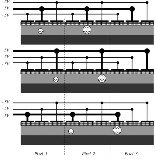
During the readout phase, the charges are transferred from pixel to pixel on the columns – it is called the shift. This process is performed by sequentially changing the voltage of electrodes, since the negative charges follow the most positive potential (see figure 3.1):
Figure 3.1: The shift of charges in CCD
3.1.2 The CCD cameras architectures
There are three main architectures for CCD cameras.
The Full Frame CCD
Nearly all the sensor area is used to collect photons so this architecture is very sensitive. The accumulated charges in the image area are shifted vertically, all the row simultaneously, by one pixel. Therefore, the bottom line of the image is transferred into the horizontal serial register. Then the horizontal serial register is shifted horizontally to the read-out circuit where each individual pixel is amplified by a common gain and read-output to the A/D converter (or to the modulator if we want an old-style analog TV signal). The main disadvantage of a full frame sensor is the charge smearing caused by light falling on the sensor whilst the read-out process. To avoid this, a mechanical shutter is used to cover the sensor during the read-out. The shutter is not needed when a pulsed light source is used.
- 5V 5V - 5V - 5V - 5V 5V 5V - 5V - 5V
Pixel 1 Pixel 2 Pixel 3
35
Figure 3.2: The full frame architecture
The frame transfer CCD
A storage area is added between the image area and the horizontal serial register (figure 3.3). The storage area has the same dimension as the image area and is protected from light by a light-tight mask. When the exposure time is over, the accumulated charges in the image area are shifted quickly to the storage area. While the storage array is read, the image area can accumulate charges for the next image. A frame transfer CCD imager can operate continuously without a shutter at a high rate. The sensor circuit is bigger and then more expensive than the full frame sensor since the storage area is approximately as large as the active area. The fill ratio of the active area is very good, nearly 1, like for the full frame sensor.
Figure 3.3: The frame transfer architecture
The Interline Transfer CCD
The interline-transfer CCD has charge transfer channels called Interline Masks (the gray area in the figure 3.4). These are immediately adjacent to each photodiode. They play the
Image area Horizontal serial register Read-out Image area Storage area Horizontal serial register Read-out
36
same role as the storage area of the frame transfer CCD, but since they are very close to the accumulation regions, the accumulated charges can be rapidly shifted into the channels after the exposure time. The very rapid image acquisition virtually eliminates image smear. The disadvantage of interline transfer architecture is the interline mask reduces the light sensitive area of the sensor as is decreases the fill ratio.
Figure 3.4: The interline-transfer architecture
3.2 Quantification of the signal provided by our camera
Our EMCCD camera is a frame transfer camera, but with the addition of a programmable gain. We now explain how we use it and how we studied the histograms of the data collected from the camera. With these diagrams, we developed a numerical method to calculate the average number of photoelectrons at the input of the multiplying register. Therefore, we can estimate the average number of photons incident on the camera sensor.
3.2.1 Theory
In the EMCDD camera, after the exposure process, the photoelectrons in the image area move quickly to the storage area. Then the charges in the pixels of each row are shifted to the horizontal serial register line by line. This process is similar to the one in an ordinary frame transfer CCD. The difference is that those charges are multiplied by a multiplication register before they reach the readout circuit (figure 3.5).
The multiplication register contains many hundreds of cells that are driven with a sequence of voltage to move the charges to the next element. An avalanche multiplication of the electrons occurs as they are moving through each element of this register. The gain per cell is actually quite small, only around 1.01–1.015. Nevertheless, with a large number of cells, a substantial total mean electron multiplication gain G is achieved. To ensure a good dynamic range and gain stability, among other considerations, the actual gain is normally no bigger than 1000.
Image area
Horizontal serial register
37
Figure 3.5: EMCCD architecture
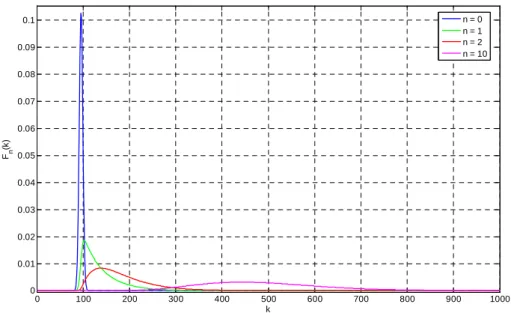
Due to the stochastic nature of the multiplication process, each photoelectron, which passes through the multiplication register, has different gains from the other photoelectrons. As a result, a large range in the number of output charges could be produced from each possible number of input photoelectrons n. The distribution of output charges m can be approximated by the formula 3.1 [66]
( )
( )
0 0 ! 1 exp 0 1 = = > − − = − n n n G G m m m T m n n nδ
(3.1)where δ0m is the Kronecker delta
If the Analog to Digital Conversion (ADC) process is perfectly linear, each small set of m values will correspond to a digital value k, and we could rewrite the formula 3.1 to
( )
(
)
0 0 ! 1 exp 0 1 = = > − − = − n n n g g k k k f k n n nδ
(3.2)fn(k) is the histogram that corresponds only to n photoelectrons entering the electron multiplying register, and g is a constant number. In other word, the probability to obtain the value k at the output of ADC is fn(k) for n input photoelectrons.
In the fact, the ADC process is not perfect. When there are no input charges, we have the Gaussian-shape histogram
Image area Storage area Horizontal serial register Multiplication register Read-out