HAL Id: hal-00862938
https://hal.archives-ouvertes.fr/hal-00862938
Submitted on 17 Sep 2013
HAL is a multi-disciplinary open access
archive for the deposit and dissemination of sci-entific research documents, whether they are pub-lished or not. The documents may come from teaching and research institutions in France or abroad, or from public or private research centers.
L’archive ouverte pluridisciplinaire HAL, est destinée au dépôt et à la diffusion de documents scientifiques de niveau recherche, publiés ou non, émanant des établissements d’enseignement et de recherche français ou étrangers, des laboratoires publics ou privés.
Structuring and integrating human knowledge in
demand forecasting: a judgemental adjustment approach
François Marmier, Naoufel Cheikhrouhou
To cite this version:
François Marmier, Naoufel Cheikhrouhou. Structuring and integrating human knowledge in demand forecasting: a judgemental adjustment approach. Production Planning and Control, Taylor & Francis, 2010, 21 (4), pp.399-412. �10.1080/09537280903454149�. �hal-00862938�
Structuring and integrating human knowledge in demand
forecasting: a judgmental adjustment approach
François Marmier1,2
and Naoufel Cheikhrouhou1*
1
Ecole Polytechnique Fédérale de Lausanne (EPFL), Laboratory for Production Management and Processes, Station 9, CH-1015, Lausanne, Switzerland.
2
Université de Toulouse, MINES ALBI – CGI, 81013, Albi, France. * corresponding author: [email protected]
Abstract
Demand forecasting consists of using data of the past demand to obtain an approximation of the future demand. Mathematical approaches can lead to reliable forecasts in deterministic context through extrapolating regular patterns in time-series. However, unpredictable events that do not appear in the historical data can make the forecasts obsolete. Since forecasters have a partial knowledge of the context and of the future events (such as strikes, promotions) with some probability, the idea presented in this work is on structuring the implicit as well as the explicit knowledge in order to easily and fully integrate it in final forecasts. This paper presents a judgemental-based approach in forecasting where mathematical forecasts are considered as a basis and the structured knowledge of the experts is provided to adjust the initial forecasts. This is achieved using the identification and classification of four factors characterising events that could not be considered in the initial forecasts. Validation of the approach is provided with two case studies developed with forecasters from a plastic bag manufacturer and a distributor acting in the food market. The results show that structuring the expert knowledge through the identification of factor-related events lead to high improvements of forecasts accuracy.
Keywords: Forecasting; Demand planning; Judgemental forecasting; Judgemental factors; Time
series
1 Introduction
Demand planning and forecasting using time series consists of using historical data of the past events to obtain an approximation of the future demand. Many ways of developing forecasts have been studied and proposed such as the different mathematical and statistical methods (Makridakis and Hyndmann 1998). Although mathematical approaches can lead to reliable forecasts in some contexts, extrapolating regular patterns in series to predict specific events can render the forecasts obsolete. On the other hand, forecasters have as an asset their partial knowledge of the context and potential external stunner. This knowledge is not available within the statistical methods as it corresponds to special events, such as personnel strike or limited promotions on products. Nowadays, it is recognized that judgment is an indispensable component of forecasting (Lawrence et al. 2006) and that there is still a need for studies which could help companies to improve their forecast quality using contextual information (Meunier Martins et al. 2007, Sanders and Ritzman 1995,). In the context of high uncertainty, it is beneficial to integrate efficiently judgmental and mathematical approaches in order to take advantage, on the one hand, of the capacity of the company‟s actors to anticipate changes and integrate domain knowledge, and on the other hand of the strength of mathematical models. Meunier Martins et al. (2005) take the judgement into account in the upstream part of the forecasting process in order to define the priorities, whereas Franses (2008) considers the integration of contextual information in the
downstream part, where different combinations of judgemental and mathematical forecasts are possible.
The objective of this work is the development of a methodological approach for the improvement of forecasting accuracy by structuring and efficiently exploiting expert knowledge. A judgmental adjustment based approach, combining mathematical forecast and judgmental factors, is discussed and its performance is compared to classical mathematical forecasting techniques. In the judgmental adjustment based approach, mathematical forecasting is applied in order to give initial forecasts. Based on judgemental factors, identified and presented in this work, the expert structures his/her knowledge related to the industrial and commercial context and adjusts the mathematical forecasts previously obtained. The forecasting accuracy of the developed approach is compared to forecasting accuracies of other different methods is done using common error measures. Furthermore, the approach is validated and criticized with the help of a plastic bag manufacturer in the southern area of Spain and a distributor in the north of France.
In Section 2, an overview through the literature of the features of the forecasting techniques, integrating judgemental methods, is presented and discussed. Section 3 outlines the details of the proposed judgmental adjustment based approach and its main features. The error measures used to assess the quality of the approach is proposed in section 4. Two industrial case studies using the developed approach related to the plastic bag and the distribution markets are presented in section 5. Finally, Section 6 provides the conclusions of this work and future research directions.
2 Combined judgemental-mathematical forecasting systems
Forecasting integrating the expert judgment has mainly to deal with three research work families: a- the modification of the historical data series to take into account the knowledge of the contextual information,
b- the achievement of forecast which can be based on results of mathematical approaches and c- the adjustment of the forecasts to anticipate the impact of known events (Webby et al. 2005). Webby and O‟connor (1996) define four main types of approaches integrating human judgment into structured forecasting methods: the model building approach is a methodology which uses judgment in the selection and development of the quantitative forecast (Bunn and Wright 1991). The forecasts are obtained through the combination of judgemental and mathematical forecast requiring for that high technical knowledge. This combination is a pragmatic approach for integrating the personal analysis of contextual information that may influence the forecasts (Fildes and Goodwin 2007). Sanders and Ritzmann (1995) show that it gives good results for time series with low variation coefficient. Moreover, both (mathematical and contextual) forecasts have to present similar accuracies in order to ensure reliable global forecast.
The judgemental decomposition consists of identifying and analysing the effects of past contextual information in time series before establishing mathematical forecasts. Once the mathematical forecasts are achieved, factors related the future events are taken into account and the forecasts are then adjusted judgementally (Edmundson 1990). Judgemental decomposition is more complex than combination or adjustment methods, but it may bring a good structure when integrating judgement into forecasting. From the planner point of view, it is possible that decomposition reduces the cognitive workload, but it may also be risky and ineffective in certain circumstances. Indeed, the multiplicative reconstruction of decomposed components increases the risk of errors and thus, good results are not guaranteed. In the judgemental adjustment process, the mathematical forecasts are reviewed by forecasters/experts and then adjusted on the basis of their knowledge and experiences. Judgemental adjustment of mathematical forecasts is a common practice in companies and it constitutes the major competing alternative to the combination process for integrating judgement into forecasts. However, the practice of judgemental adjustment is criticised because of its informal nature (Bunn and Wright 1991); Using a
procedure or a decision support system to structure information is helpful in both decision making and forecasting. Judgemental adjustments lead to improvements in accuracy when the process is structured. For instance, forecasters should comment and/or explain how they adjust the forecasts and on which basis this is done. With this method, the forecasting process is performed sequentially with the quantitative forecasts firstly generated which are then adjusted, based on the different available judgments. Sanders and Ritzmann (2004) report the advantages of this approach of which is time reduction, allowing the judgment to rapidly incorporate the latest updated information. Flores et al. (1992) compare different approaches of judgemental adjustment; The forecaster ranks the impacts due to different factors to obtain an average adjustment of an ARIMA forecast. Similarly, Lee et al. (1990) define different event-based factors to determine the reaction of the demand in different situations. These factors are used in a case based reasoning system which plays the role of forecasting expert.
In order to integrate human judgment factors in mathematical models, this work proposes a factor-based approach to assist the forecaster in focusing selectively on different events and in structuring his judgment when adjusting forecasts. Therefore, the forecaster will be able to communicate easily his implicit knowledge concerning the future evolution of the markets (total volume, number of competitors…), the customers (their number, needs, potential demand…) and the contractors (development status, special offers…) by representative factors. Afterwards, the expert weighs the impact of the future events and adjusts the mathematical forecast.
3 Proposed approach
The global approach consists of integrating the expert judgement in a structured manner as complementary information to mathematical forecasts, established by means of classical mathematical methods.
[insert figure 1 about here]
Figure 1 describes this approach composed of three steps: first, data are filtered (cleaned) and initial mathematical forecasts are developed. Second, different event-based factors are identified and determined by experts and the factor variables are weighted. Third, the mathematical forecasts are adjusted with the variable values.
3.1 First step : data filtering and mathematical forecasting
This step consists of identifying the outliers and removing the effect of non periodic events on the time series. The latter is decomposed, taking into account past contextual information. In other words, the actual data Y t( k) of the time-series Y t( ) is modified when necessary in order to
become filtered (noted YO(tk)), k= K,…,0. In fact, some outliers could exist in time series as
unusual or erroneous data observations. They may be examined and analysed in detail by the forecaster or the salesman in order to decide on keeping or deleting them from the time-series. These abnormal values are often observed in the gross market segment. For instance, an advertising campaign could cause an abnormal increase in demand whereas a strike in transportation companies could cause an abnormal decrease of demand. Outliers can also result from data entry errors and are frequently encountered in industrial databases.
Testing the existence of an outlier and removing it consists of verifying whether the corresponding value in the time series belongs to a calculated confidence interval, calculated with respect to the desired forecasting accuracy. Every observation of the time series which is outside of this interval is rejected and replaced by another representative value, for instance, by the average of the neighbouring values. If the time series presents a strong trend or a seasonal pattern,
this test is not adequate and should not be adapted. In that case, a confidence interval is evaluated for each year and each time period. An observation is considered as abnormal if it is outside both of the "yearly" and of the "periodical" confidence interval. In the case a time series presents a strong trend, the test is made after removing the trend. Thus, the mathematical forecasts for the given filtered or “cleaned” time-series are defined in Equation 1.
^ 0( ) ( O( 1), ( O( 2), ...) Y t f Y t f Y t (1) Where ^ 0( )
Y t is the forecast based on cleaned data for the period t.
3.2 Second step: Identification and formalization of influencing factors
A judgmental factor is defined as a “factor that cannot be fully incorporated into the time series models, and thus cannot be effectively identified by the extrapolation of past patterns in the data set” (Lee and Yum 1998). The attributes or causal variables are the variables that cause changes to the factors. They are defined depending on the particular studied case. The different attributes could be: duration, intensity, type, etc. The realization of judgmental factor is considered as a judgmental event. Thus, a judgmental event is accompanied by its impact and may affect the demand over more than one time period. In addition, judgmental events can cause different types of judgmental factors. So, the judgmental event impact is calculated over the relevant instance periods.
The common characteristics of judgmental factors for which they are considered in the forecasting process are:
The factors occur irregularly and infrequently. Thus, the amount of data considered is usually too small for statistical modelling and evidence,
The impact is too significant to be neglected,
The effect can be transient or can change the forecasts in a considered way over time with respect to the original data characteristics,
The occurrence of the related coming events can be identified in advance by experts even if it is difficult to judge their impacts with precision.
These factors are grouped into 3 different categories related to:
The markets: external factors influencing the market and characteristics of the market, volume, competitors,
The clients: needs, development status,
The contractors: offers, product characteristics, prices, quality and design.
The type of judgmental factors may vary from an activity sector to another (Lee et al., 1990). The judgmental factors considered in this work consist of 4 types: transient factors, quantum jump factors, transferred impact factors and trend change factors. Each factor is the consequence of a causal variable allowing the experts to make the adequate adjustments of the initial forecasts. Each adjustment has an impact on the initial forecast over time. Each adjustment, resulting of a judgmental factor is noted F(i,t) where F is the adjustment value, i is the total impact and t is the time. The impact i can reach its maximum value m a x
. The expert expresses his opinion by weighting m a x
with a weight w, chosen using the following impact scale from 1 to 5: 1- Highest: 80 <w<100%.
2- Higher than normal: 60<w<80%. 3- Normal: 40<w<60%.
4- Lower than normal: 20<w<40%. 5- Lowest: 0<w<20%.
Then :
i = w.m a x (2)
3.2.1 Transient factors
The transient factors influence time series data only during the period in which a particular event occurs (cf. figure 2), such as a strike. When the event is over, the effect does not last any longer. Therefore, the effect of transient factors can be removed explicitly from the time series data. Moreover, the detection of outliers can be useful in identifying the different transient factors that could be related to.
[insert figure 2 about here]
Assume that time can be decomposed into periodical instances tp (p =1…n). The total impact i
covers the effective number of impacted periods (t1…. tn.). Adjustments encompassing n
consecutive periods p are calculated by equation 3 :
1 ( , ) ( , ) n p p p F i t f i t
(3)Where f are the periodical adjustments and ip corresponds to the intensity of the impacted period
tp.
Transient factors can decrease or increase the value of the main initial trend
^ 0
Y . The expert establishes first the sign of the adjustment (positive or negative). Then, the maximum value of the adjustment m a x
is estimated and finally, according to his/her knowledge, the expert deduces the weight w in order to obtain the total impact.
3.2.2 Transferred impact factors
The global impact i of this kind of event is transferred from one set of periods Sp1 to another set
Sp2 ,without changing the global forecasts of the related consecutive periods. Figure 3 shows an
example of this factor. This phenomenon is observed, for instance, when price changes are announced beforehand at time ta. In this case, the temporary change in demand due to the
expected price change is transferred and compensated in the following time period at time te.
Then, Sp1 precedes Sp2. But if ta = te, Sp2 precedes Sp1. This is a common situation when suppliers
want to reduce their inventories and thus proceed to special offers for their customers. [insert figure 3 about here]
Periodical instances that encompass n consecutive periods are calculated in (4):
1 ( , ) ( , ) n p p p F i t f i t
(4)where ip is the proportional impact (positive or negative) of the factor during the time period p.
Similarly to the other factors, the expert determines the maximal value m a x
to be transferred and uses the scale of impact to rate the event and to obtain i as shown in equation 2.
3.2.3 Quantum jump factors
The quantum jump factor, as presented in figure 4, occurs when the effect of a non-repetitive event is permanent. When time series models cannot implicitly forecast a quantum change, it will be effective to consider the impact explicitly for a while.
[insert figure 4 about here]
These factors can be detected by identifying if the magnitude of a demand shift from the previous period of the same year, or from the same period of the previous year, exceeds a fixed threshold. The detection criteria considered by the forecaster are then:
1 ) 13 ( ) 12 ( ) 1 ( ) ( t Y t Y t Y t Y AND 2 ) 13 ( ) 1 ( ) 12 ( ) ( t Y t Y t Y t Y
Where α1 et α2 are threshold values. Events can be determined by reviewing the past events at the
detected time and computing the forecast error.
The adjustment created by a quantum factor is evaluated and separated in different instances in order to be integrated to the original mathematical forecast. This adjustment is detailed in equation 5.
( , ) .
F i t i Q j (5)
Where Qj is a binary variable which meaning that the Y-intercept, which define the elevation of the demand trend, is impacted by the intensity i at te, the effective date (date of the jth event that
generates the demand jump). If t < te then Qj =0
Otherwise Qj =1.
The weighting process of the jump factor variables is similar to the one of the other factors. After determining the adjustment sign, the expert has to determine the maximal value of the adjustment
m a x
and expresses his /her opinion about the percentage that weights that variable. In other words, the forecaster expresses his/her implicit knowledge regarding the factor, using the previous impact scale to obtain i.
3.2.3 Trend change factors
Some factors such as price variation can modify the demand by a percentage. These factors are considered as trend change factors as shown in figure 5. Most of the time, the price change is known a priori, and it is possible to forecast the trend change. If the expert provides contextual information, a regression of ( ) ( 1) Y t Y t on ( ) ( 1) P t
P t can estimate the impact of price changes, where P(t) is the price at time t. Otherwise, the expert establishes the sign of the possible trend change
and its limit m a x
. Then, he/she weighs the impact using the impact scale. The trend adjustment is detailed in equation 6.
[insert figure 5 about here]
( , ) . .
F i t i t T c (6)
Where Tc is a binary variable which meaning that the slope of a linear regression of the demand trend is impacted with the intensity i at te, the effective date (the date of the event generating the
demand jump):
If t < te then Tc =0
3.3 Third step: the adjustment process
The final adjusted forecast is defined as:
^ a
Y
(t) = ^ o Y (t) + ^ Y (t) (7)Where ^Y (t) is the adjustment calculated with the judgmental factors expressed by the experts.
It corresponds to the total impact on demand of the different events occurring at time t. Some factors influenced the demand over a restricted period or a set of periods but others are definitely modifying the demand behaviour. When multiple judgmental factors impact simultaneously the demand, it is necessary to take into account forecast adjustments according to the effects of each individual judgmental event. Then, the global adjustment at time t, defined by equation 8, corresponds to the sum of the different adjustments related to the K factors impacting the demand at time t : ^ 1 ( ) , K k k k Y t F i t
(8)4 Evaluation of adjusted forecast quality
Accuracy plays an important role in evaluating forecasting methods and demand planning, since it measures how well the results of the forecasting model correspond to the actual data. Different methods usually lead to different measures of accuracy. Since accuracy is an important measure in forecasting, it is important to understand their strengths and weaknesses in order to select the appropriate measure for a given context. In the following, Yt is the actual value at period t and Ft
is the forecast value for this period.
Forecast accuracy is evaluated using different error measures. In general, the error measure used should be the one that is most closely related to the decision being made. The simplest is the Forecast Error (FE) (cf. equation 9) or the Percentage Error (PE) (cf. equation 10). Some commonly used error measures are Mean Absolute Deviation (MAD), Mean Absolute Error (MAE) (cf. equation 11), Mean Percentage Error (MPE), Mean Square Error (MSE) and Root Mean Square Error (RMSE), R2 (or R-squared), Mean Absolute Percentage Error (MAPE) (cf. equation 12). The selection of a measure depends on the purpose of the analysis.
FE for a period t is the difference between the actual and the forecast values of the considered period. PE does not provide the error measure in the units used in the original data. Armstrong (2001) alleged that R2, which assesses the pattern of the forecasts relative to that of the actual data is not particularly useful to forecasters with business expertise and its use is probably more harmful when using time-series data. Moreover, he demonstrates that MSE should not be used due to its unreliability in explaining the results. Like MSE, RMSE penalizes errors according to their magnitude. Both MSE and RMSE are not unit-free and therefore comparisons across series are difficult. On the other side, there is no way to know how MAD error is large or small with respect to the actual data. With the ME and MPE measures, the real significance of the error can be difficult to evaluate because errors can be annulated when summing negative and positive components. Contrary to ME, the use of MAE makes it possible to highlight both positive and negative errors. With MAE, the total magnitude of error is provided but not the real bias or direction of the error. MAPE measures the deviation as a percentage of the actual data with respect to the forecast. Thus, positive and negative errors do not cancel out.
In this paper, MAE and MAPE are used to calculate the forecast errors as they are considered as being the most performing approaches to measure errors.
t t t Y F e (9) Percentage Error: t t t t t t Y e Y F Y PE (10)
Mean Absolute Error:
n t e n MAE 1 (11)Mean Absolute Percentage Error:
n t t t t n t Y F Y n PE n MAPE 1 1 1 (12)5 Industrial data applications
The practical usefulness of the proposed forecasting approach is shown in this section by means of two real industrial case studies: a plastic bag manufacturer and a distributor on the food market. In both cases, a forecasting expert proceeds to structuring and integrating his implicit knowledge into mathematical models.
5.1 Presentation of the first case study
This approach is applied to the case of the Company X, a plastic bag manufacturer based in the south of Spain. The polyethylene bag market is analyzed and the demand is forecasted. The time series used are composed of the aggregated monthly demand collected over three years (2004-2006), as it can be observed in figure 6. The aim of this study is to plan the demand for the year 2007. Company X has three main customers in this area which are supermarkets. The expert will analyze the historical data and the influencing factors in the plastic bag demand and forecast the specific events relying on his knowledge.
[insert figure 6 about here]
The first step consists of cleaning the data. The time-series presents a strong trend which has to be removed during the cleaning process of the series and to be reassigned afterwards. Actually, once the trend is removed, it is possible to identify more easily the outliers. These outliers have to be deleted and replaced by a significant value in order to obtain “cleaned” time-series relevant to the identification of demand patterns. The forecasting process is then applied to the cleaned time-series which keep the same information on trend and seasonality. The way outliers are identified and deleted consists of verifying if a value from the time series belongs to a confidence interval
IC given by equation 13. Y Y IC 1.96 (13) where Y
is the average value of the time series over a considered horizon, y is the standard
deviation of the corresponding observations and 1.96 is the corresponding reduced centred variable value of the normal distribution for a confidence level with an error probability of 0.05.
In this case, one outlier is observed for t = 29 months. This observation, which is outside the confidence interval, is considered as abnormal and is replaced by the average of its two neighbouring values. The cleaned data series is presented in figure 6.
5.2 Initial mathematical forecasts
The time-series present a strong trend as shown in figure 6. Moreover, a weak seasonality is observed in the historical data. This seasonality is due to the demand increase of plastic bags during the months before summer and Christmas holidays. Even if seasonality is well identified for this time series, longer observations with at least 4 years (for monthly series) are needed to ensure the existence of seasonal variations.
It is possible to eliminate several models which are devoted to particular behaviour of data series such as the simple linear regression that implies that no seasonal variation exists. The moving average and simple exponential smoothing implies that neither seasonal variation nor tendency exists. In addition, the data-series can not be assimilated to a random process (such as random walk), because of the observed seasonality and trend. Because it takes into account all the factors characterizing the demand, we propose here to use an Autoregressive Integrated Moving Average (ARIMA) model. The latter assumes that the best forecast is given by a parametric model relating the most recent data to the previous data and noise (Box et al. 1994).
The ARMA Add-in for Excel is used to compute the ARIMA(p,d,q) model and to identify the best parameters p, d, and q. These parameters are defined as integers greater than or equal to zero, referring to the order of the autoregressive, integrated, and moving average parts of the model respectively. The figure 7 presents the forecasts obtained with the ARIMA(5, 0, 4) method for the period 2006-2007.
[insert figure 7 about here]
5.3 Subjective adjustments
The forecasting expert of the company X has to identify and classify the different factors as transient, transferring, jump or change trend factors before proceeding to weigh them. Thanks to this classification, the adjustment can be made. In this case study, the expert proposes that the following factors would affect the demand in the forecasted year:
Plastic price: Since supply and demand determine the price and the quantity, when plastic prices
increase, the clients will ask for lower quantities. It corresponds to a trend change factor. In this case, the expert predicts that the trend of the demand is going to change since the raw materials price will increase from January 2007 due to new framework contracts. The plastic price is then the causal variable related to that factor.
The trend can be computed with the method of the least squares, with a regression line. Expert has then to weight how much the trend line is going to change. Assume that P(t) is the price at and Y(t) is the demand at time t. A regression of ( )
( 1) Y t Y t on ( ) ( 1) P t
P t estimates the impact of
price changes as shown in equation 14,
( ) ( )
Y t a b P t (14)
The process to adjust the trend is the following: 1. Straighten the forecast by removing the trend.
2. Compute the price impact and the new trend. 3. Add the new trend to the forecast.
In developing a regression analysis based on his/her own knowledge, the expert identifies that the trend is going to get a value of approximately -4. After this adjustment, the overall (judgemental and mathematical) forecast is shown in figure 8.
[insert figure 8 about here]
The different trends of the time series including the mathematically forecasted trend are shown in figure 9. As shown, the consequence of the factor „price change‟ of the raw material would be a decrease of the trend slope of 1.6° during the 12 forecasted months.
[insert figure 9 about here]
Special offer: The expert predicts that the company X will have too much stock in the beginning
of the year 2007. A special offer to their clients is then planned, consisting of delivering the double quantity with lower price. The consequence of this factor is that a major part of the demand of January will be transferred to February and March 2007. In this case, the special offer is classified as a transferring factor. This factor depends on the proposed price in the special offers and on the holding costs.
The special offer is made to the four main customers. The expert weighs the causal variable of the special offer that the company makes. He takes into account the potential of each customer and estimates the weight of their potentials. The process is then:
1. Classifying the different clients to which the offer is made.
2. Analyzing their inventory capacities and their interests in the special offer.
3. Weighting each client‟s interest according to the different percentages: 0-20%, 20%-40%,
40%-60%, 60%-80%, and 80%-100%.
4. Applying the percentages to each client‟s special offer.
The results of the expert rating in table 1.,show that he/she predicts a demand increase for Client 1 and Client 2 in January. This means that the demand forecast in January will increase and the one in February and March will decrease.
[insert table 1 about here]
Plastic bag improvements: Nowadays, large companies take care of fulfilling different
environmental requirements. Effective tools for the analysis of environmental aspects of an organization and for the generation of options for improvement are provided through the concept of Cleaner Production. In this frame, Company X is willing to make technical changes in their plastic bags and improve the raw materials in order to fulfil the ISO 14000 requirements. The expert predicts that using ecological non-polluting plastic bags is an interesting Marketing criterion for supermarkets. Thanks to this technical improvement in plastic bags, the demand would increase. This factor is classified as a jump factor since there would be new clients willing to try this new concept of plastic bags. Here, the causal variable is the demand volume of the new client interested in the ecological plastic bags.
Company X received offers from a potential client (Client 5) just in case they offer biodegradable plastic bags. The company decided to make an experimental change in their raw materials based on a new generation of biodegradable substances, during the two months of summer.
The expert expects that this change will not affect current clients but rather those companies interested in ecological issues. For this weighting causal variable, the expert rates the client‟s
interest as shown in table 2. In this case, only the new client (Client 5) is interested by the new material. The demand of the other customers is not influenced by the technical improvements.
[insert table 2 about here]
Client situations: Company X has a client (Client 3) that asks regularly for a fixed quantity of
plastic bags per month. This client announced that its facilities are going to close during a month after the summer holidays for maintenance purposes. The consequence of this event will be a decrease in the total demand. However, this client will order new plastic bags for November. This case shows the importance of the relationship between the client and the supplier and the role of human factors in demand planning. This factor will be classified as a transient factor, because it is an unusual event that provokes an outlier in the forecast demand. Thus, the client‟s demand volume is the causal variable that creates the demand change. Table 3 shows the weight of this variable.
[insert table 3 about here]
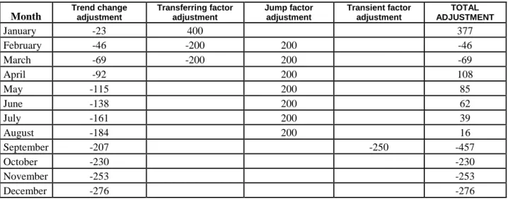
Table 4 presents the total impact of the different considered factors on demand per month using the information from tables 1-4.
[insert table 4 about here]
5.4 Adjusted forecasts
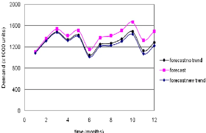
Figure 10 compares the real 2007 sales data to the mathematical forecast and to the judgmentally adjusted forecast.
[insert figure 10 about here]
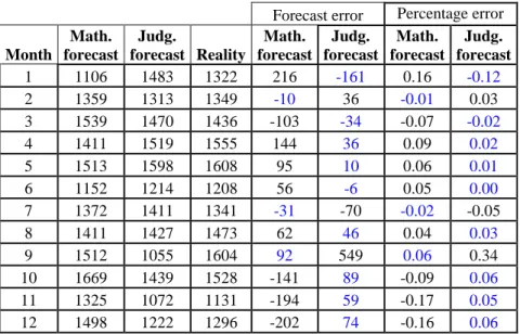
Table 5 gives for each forecasted month the forecast error in product units and in percentage. It is clear that adjusted forecasts present better results compared to the initial mathematical forecasts, since it gives results closer to the real sales in 9 months over 12.
[insert table 5 about here]
Table 6 presents the forecast performances of the proposed approach, measured using MAE and MAPE. The adjusted forecast gives the best results since the MAE has been decreased by 14% and the MAPE by 18%. In addition, the MAPE is about 0.06 meaning that, in average, only a global error of 6% has been made on the forecasted year.
[insert table 6 about here]
The historical data series used to approximate the future demand do not contain the impact of non periodic events, such as those that could be related to the four identified factors. Therefore it can not logically lead to optimal forecasts. Adjustments help only to minimize the forecast errors. Forecasts seem logically improved because the achieved adjustments are based on the expert knowledge. However, if adjustments were done globally, without structuring or without a real analysis of their impacts, of their durations and of their expanses over time, the deviation and the error could increase. Such approach has to be sufficiently simple to be usable, but also complete to allow representative adjustments with respect to the industrial reality. This case study shows the efficiency of adjusted forecasts integrating structured human knowledge, proving that the integration of structured human knowledge in forecasting leads to beneficial results.
5.5 Second case study
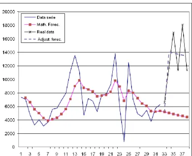
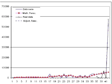
In this second application, we are interested in a set of 4 different products provided by a fresh food distributor with historical sales on different horizons (from 20 to 36 months) depicted on figures 11 to 14. The objective is to forecast the demand on a horizon of 6 months for all of the considered products. For the different time series, the expert identifies that mathematical forecast would not be sufficient to achieve reliable forecasts. Different factors due to customers‟ demand behaviour are considered without detailing the causal variables (several exceptional high orders have been already announced by their customers). First, mathematical forecasts are generated on an horizon of 6 months, through the identification of the best models fitting the historical data (double exponential smoothing for the series shown in figures 11, 12 and 14 and Holt-Winters for the series of figure 13). The forecasts are then adjusted by a salesman using the proposed procedure and reported on the different figures. The difference between mathematical forecasts and real sales shows the limit of the past data extrapolation to obtain reliable forecast (cf. Fig. 11 to 14); By using the structured expert judgement (jump factor for the case on figure 11, transient factor on several time periods on figure 12 and two transient factors on figures 13 and 14), substantial improvements of the forecast accuracy are achieved.
[insert figure 11 about here] [insert figure 12 about here] [insert figure 13 about here] [insert figure 14 about here]
Table 7 shows the improvement of the forecast accuracies relying on the error measures MAE and MAPE and expressed in percentage with respect to the performances of the respective mathematical models. The resulted adjusted forecast presents better results considering both the MAE and MAPE since for each product, at least an increase in forecast quality of 20% is obtained, reaching in some cases about 70%. As a conclusion, this case study further proves the efficiency of the global approach to deliver forecasts with high accuracy as shown in the first case study.
It is clear that the historical data used to approximate the future demand do not encompass the impact of non periodic events. Therefore, the adjusted forecast logically leads to improved forecasts.
[insert table 7 about here]
6 Conclusions
We propose in this paper a factor-based approach to assist the forecaster in structuring his/her judgment when adjusting forecasts. Therefore, the forecaster is able to structure and communicate his knowledge concerning the evolution of the markets, the customers and the contractors using representative factors. The global approach consists of three steps: data filtering and mathematical forecasting, factors formalization and adjustment process. Results provided via mathematical models are compared to the ones achieved through judgmentally adjusted forecasting.
This approach is applied to plan the demand of an industrial company and a distributor. It allows forecasters to identify different factors in order to integrate specific events and assess their impacts on demand forecast. For both presented case studies, the proposed approach has a
substantial impact on the accuracy of the resulting forecasts. In fact, it is noticed that the Mean Absolute Error and the Mean Absolute Percentage Error have been both decreased.
The proposed methodology is simple and complete thus, allowing the expert to transcribe each possible situation. Its originality resides in centring the forecasts around a structured expert judgement and knowledge. This approach is opposed to previous work where additional information is extracted from data in order to be integrated in different decision support systems. Different possible perspectives are considered, particularly in studying individual expert perceptions in collaborative forecasting frameworks and their contributions to the forecasting process. In fact, different experts could have different perceptions of a same factor, leading to a range of different evaluations for a same factor. In addition, further investigations are made for the improvement of accuracy obtained when the expert has a feedback based on the comparison between the adjusted forecasts and the real sales.
7 Acknowledgements
The authors thank the industrial partners for their collaboration in the achievement of this work.
8 References
ARMSTRONG J.S., 2001, Judgmental Bootstrapping: Inferring Experts' Rules for Forecasting. In J.S. Armstrong (Ed.), Principles of forecasting, p. 171-192.
Box, G. E. P., Jenkins, G. M., and Reinsel, G. C. 1994, Time Series Analysis, Forecasting and Control, 3rd ed. Prentice Hall, Englewood Clifs, NJ.
BUNN D. and WRIGHT G., 1991, Interaction of judgmental and statistical forecasting methods, issues and analysis. Management Science. 37 (5), 501-18.
EDMUNDSON R. H., 1990, Decomposition; a strategy for judgemental forecasting. Journal of Forecasting, 9 (4), 305-314.
FILDES R., GOODWIN P., 2007, Good and bad judgement in forecasting: Lessons from four companies, Foresight, 8, 5−10.
FLORES B.E., OLSON D.L., WOLFE C.,1992, Judgmental adjustment of forecasts: A comparison of methods, International Journal of Forecasting, 7 (4), 421-433.
FRANCES H. P., 2008, Merging models and experts, International Journal of Forecasting Volume 24, Issue 1, 31-33.
LAWRENCE M., GOODWIN P., O‟CONNOR P. and ÖNKAL D., 2006, Judgmental forecasting: A review of progress over the last 25years. International Journal of Forecasting, 22, 493-518.
LEE J.K., OH S.B. and SHIN J.C., 1990, UNIK-FCST: Knowledge-Assisted Adjustment of Statistical Forecasts. Expert Systems With Applications, 1, 39-49.
LEE J.K. and YUM C.S., 1998, Judgmental adjustment in time series forecasting using neural networks. Decision Support Systems, 22, 135-154.
MAKRIDAKIS S. and HYNDMANN R.J., 1998, Forecasting, methods and applications. John Wiley & Sons, Inc. Third Edition, 185-240.
MEUNIER MARTINS S., CHEIKHROUHOU N., GLARDON R., Strategic analysis of products related to the integration of human judgment into demand forecasting, Integrating Human
Aspects in Production Management. ZÜLCH, Gert; JAGDEV, Harinder S.; STOCK, Patricia (Eds.): New York: Springer, 2005.
MEUNIER MARTINS S., WINDISCHER A., MATHIER F., CHEIKHROUHOU N., GLARDON R. and GROTE G., A new system to improved demand forecasts based on socio-technical considerations. Accepted for publication in International Journal of Production Economics.
SANDERS N.R. and RITZMAN L.P, 1995, Bringing judgment into combination forecasts. Journal of Operations Management, 13, (4), 311-321.
SANDERS N.R. and RITZMAN L.P, 2004, Integrating judgmental and quantitative forecasts: Methodologies for pooling marketing and operations information, International Journal of Operations & Production Management, 24 (5), 514-529.
WEBBY R. and O'CONNOR M., 1996, Judgemental and statistical time series forecasting: a review of the literature. International Journal of Forecasting, 12 (1), 91-118.
WEBBY R., O'CONNOR M., EDMUNSON B., 2005, Forecasting support systems for the incorporation of event information: An empirical investigation, International Journal of Forecasting, 21 (3), 411-423.
Figure 1. Conceptual scheme of the general method developed
Figure 2. Transient factor
Figure 3. Transferred impact factor
Demand Time Demand Time Time-series Raw data Time-series “Cleaned” Filtering Mathematic forecasting ^ o Y Adjustement Events knowledge Factor identification & formalization ^ Y ^ a Y Judgmental factors Splitting Step 1 Step 2 Step 3 ta
Figure 4. Quantum jump factor
Figure 5. Trend change factor
Figure 6. Historical demand of Company X (2004-2006)
Figure 7. Company X demand (2004-2007)
Demand
Time Demand
Figure 8. Forecast without trend (2007)
Figure 9. Trend lines (2004-2007)
Figure 11. jump factor identification.
Figure 12. transient factor identification on several time periods
causal variable type weighting Weight causal variable
variable 1 Client1 capacity 60-80% 100 variable 2 Client2 capacity 80-100% 300 variable 3 Client3 capacity 0% 0 variable 4 Client4 capacity 0% 0 Table 1. Factor 2 : transferring factor
causal variable type weighting Weight causal variable
variable 1 client1 interest 0% 0 variable 2 client2 interest 0% 0 variable 3 client3 interest 0% 0 variable 4 client4 interest 0% 0 variable 5 client5 interest 80-100% 200 Table 2. Factor 3 : Jump factor
causal variable type weighting Weight causal variable
variable 1 client1 interest 0% 0 variable 2 client2 interest 0% 0 variable 3 client3 interest 100% -250 variable 4 client4 interest 0% 0 Table 3. Factor 4 : Transient factor
Month Trend change adjustment
Transferring factor adjustment Jump factor adjustment Transient factor adjustment TOTAL ADJUSTMENT January -23 400 377 February -46 -200 200 -46 March -69 -200 200 -69 April -92 200 108 May -115 200 85 June -138 200 62 July -161 200 39 August -184 200 16 September -207 -250 -457 October -230 -230 November -253 -253 December -276 -276
Forecast error Percentage error Month Math. forecast Judg. forecast Reality Math. forecast Judg. forecast Math. forecast Judg. forecast 1 1106 1483 1322 216 -161 0.16 -0.12 2 1359 1313 1349 -10 36 -0.01 0.03 3 1539 1470 1436 -103 -34 -0.07 -0.02 4 1411 1519 1555 144 36 0.09 0.02 5 1513 1598 1608 95 10 0.06 0.01 6 1152 1214 1208 56 -6 0.05 0.00 7 1372 1411 1341 -31 -70 -0.02 -0.05 8 1411 1427 1473 62 46 0.04 0.03 9 1512 1055 1604 92 549 0.06 0.34 10 1669 1439 1528 -141 89 -0.09 0.06 11 1325 1072 1131 -194 59 -0.17 0.05 12 1498 1222 1296 -202 74 -0.16 0.06
Table 5. Comparison of the forecasts and the errors for the year 2007
Measure MAE MAPE
Math. forecast 112.2086 0.081931
Judg. forecast 97.54472 0.066673
Table 6. Comparison of the error measures
Error decrease Figure 11 Figure 12 Figure 13 Figure 14
MAE 67% 38% 77% 72%
MAPE 64% 25% 20% 31%
Biographies of the authors
FRANCOIS MARMIER is graduated in Management and Production Engineering from the Ecole Nationale Supérieure des Mines de Saint-Etienne, France in 2004. After a PhD in Industrial Engineering from the University of Franche-Comté, France, in 2007, and one year as scientific collaborator at the Laboratory for Production Management and Processes at the Swiss Federal Institute of Technology at Lausanne, he becomes assistant professor in project and risk management at the Ecole des mines d‟Albi in France. His research interests include Demand forecasting, Maintenance activities scheduling and integration of human aspects in logistics, projects and services. Dr. Marmier has published several papers in various journals and international conferences.
NAOUFEL CHEIKHROUHOU is the head of the Operations Management group at the Swiss Federal Institute of Technology at Lausanne. He received his industrial engineer diploma from the Ecole Nationale d‟Ingenieurs de Tunis, Tunisia and his PhD in Industrial Engineering from the Institut National Polytechnique de Grenoble in France. His main research interests are in the areas of modelling, simulation and optimisation of supply networks, the identification and integration of human factors in production management and the reduction of management complexity in logistics and services, for which Dr. Cheikhrouhou received the Burbidge Award in 2003. Leading different projects with the collaboration of industrial partners, Dr. Cheikhrouhou has also published several papers in various journals and international conferences.