T
HEK
ALMANF
ILTER INF
INANCE:
A
N APPLICATION TO TERM STRUCTURE MODELS OF COMMODITY PRICES AND A COMPARISON BETWEEN THE SIMPLE AND THE EXTENDED FILTERSDelphineLAUTIER
CEREG1
ABSTRACT : A Kalman filter can be used for the estimation of a model’s parameters, when the model relies on non observable data. In finance, this kind of problem arises for example with term structure models of interest rates, term structure models of commodity prices, and with the market portfolio in the capital asset pricing model. The Kalman filter is also an interesting method when a large volume of information must be taken into account, because it is very fast. Last but not least, when associated with an optimization procedure, the filter provides a mean to obtain the model’s parameters. In a first section, this article exposes the basic principles of the method, shows how we can use it to estimate a model’s parameters, and presents two Kalman filters. The first one is the simple filter, which accepts only linear models. The second one, the extended filter, allows working with non-linear models. The second section is devoted to the application of the Kalman filter in finance. To explain how this method can be used in this field, we apply it to a very famous term structure model of commodity prices, and we discuss practical problems usually not mentioned in the literature, regarding the implementation of the method. The third section presents and compares the performances obtained with the two filters.
KEY WORDS: Simple Kalman filter − Extended Kalman filter − State-space models − Non observable data -−Term structure − Commodity prices − Futures prices
S
ECTION1. T
HEK
ALMAN FILTERThis section first introduces the basic principles of the Kalman filter, and explains what kind of problems this method can resolve. Then it presents the simple and the extended filters. Finally, it explains how to estimate a model’s parameters.
1.1. A brief introduction to the Kalman filter
The basic principle of the Kalman filter is the use of temporal series of observable variables to reconstitute the value of the non-observable variables. The method requires first of all that the model is expressed on a state-space form. A state-space model is characterized by a
1 [email protected]. I whish to tank Alain Galli for his advises, Totalfinaelf for the empirical data, and the French Institute for Energy for its support.
measurement equation and a transition equation2. Once this has been made, a three step iteration
process can begin.
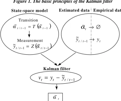
The kind of problem a Kalman filter can resolve is represented on the figure 1. The filter is useful when the model relies on variables for which there are no empirical data. The only available information for these variables α~ is the transition equation, which describes their dynamic. This equation allows the calculation of α~ in t, conditionally to their value in (t-1). Once this calculus has been made, it is possible to obtain, via the measurement equation, the measure y~ in t. This second equation represents the relationship linking the observable variables y~ with the non observable α~. The difference, in t, between the measure y~ and the empirical data y represents the innovation v. Finally, this innovation is used to obtain the value of α~at the date t, conditionally to the information available in t.
Figure 1. The basic principles of the Kalman filter
(
/ 1)
1 / ~ ~ − − = t t t t Z y α Transition MeasurementEstimated data Empirical data
1 /
~
−−
=
t t t ty
y
v
(
1)
1 / ~ ~ − − = t t t T α α State-space model∅
→
tα~
t t ty
y
/ −1→
~
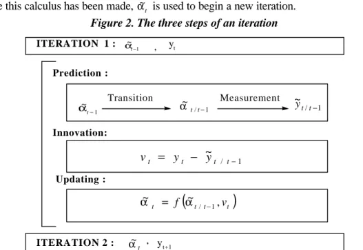
Kalman filter t α~Thus the Kalman filter allows for the calculation of α~, and updates its value when some new information arrives. There is one iteration for each observation date t, and one iteration includes three steps, as is shown in the figure 2.
During the first step, the prediction phase, the values of the non-observable variables in (t-1) are used to compute their expected value in t, conditionally to the information available in (t-1). The predictions rely on the transition equation. The predicted values α~t/t−1 are then introduced in the measurement equation to determine the measure ~yt. In this equation, the errors have zero mean and are not serially nor temporarily correlated. They represent every kind of disturbances likely to lead to errors in the data. The second step or innovation phase allows for the calculation of the innovation vt. Lastly, the values of the non-observable variables, which
2 There is more than one state-space form for certain models. Then, because, some of them are more stable than the others, the choice of one specific representation is important.
where computed in the prediction phase, are updated conditionally to the information given by vt. Once this calculus has been made, α~t is used to begin a new iteration.
Figure 2. The three steps of an iteration
ITERATION 1 : ITERATION 2 : tα y t 1 ~ − t α 1 ~ − t α α~t/t−1 / 1 ~ − t t y Transition Measurement 1 /
~
−−
=
t t t ty
y
v
(
t t t)
t f ,v ~ ~ 1 / − = α α t α~ yt+1 , , Prediction : Innovation: Updating :This presentation gives rise to two remarks. The first is that to begin the iteration process, in t = 1 for example, we need to have the value α~0. This kind of problem will be tackled in the second section. The second remark is that now it is possible to understand why the Kalman filter is a very fast method. Only two elements are actually used to reconstitute temporal series for α~ : the transition equation, and the innovation v. Because there is an updating at each iteration, the volume of information used is very low : just the new one is necessary, the one that just arrived. And once the iteration goes further, there is no need to keep it longer.
1.2. The simple Kalman filter3
The simple Kalman filter is the most frequently used version of the Kalman filter. It can be employed when the measurement and transition equations are linear.
The state-space form model, in the simple filter, is characterized by the following equations :
• Transition equation : αt/t−1=Tαt−1+c+Rηt
where αt is the vector of non observable variables in t, also called state vector, which is (m × 1),
T is a matrix (m × m), c is (m × 1), and R is (m × m)
• Measurement equation : yt/t−1=Zαt/t−1+d+εt
where yt/t−1 represents multivariate temporal series (N×1), Z is a (N×m) matrix, and d is a (N×1) vector.
t
η
andε
tare white noises, respectively (m×1) and (N×1). They are supposed to be normally distributed, with zero mean and with Q and H as covariance matrices :[ ]
t=
0
E
η
,Var
[ ]
η
t=
Q
[ ]
t=
0
E
ε
,Var
[ ]
ε
t=
H
The initial position of the system is supposed to be normal, with mean and variance :
[ ]
α0 =α~0E ,
Var
[ ]
α
0=
P
0If α~tis a non biased estimator of αt, conditionally to the information available in t,
then :
[
t −~t]
=0t
E α α
As a consequence, the following expression4 defines the covariance matrix P
t :
(
)(
)
[
~t t ~t t ']
t t E P = α −α α −αDuring one iteration, three steps are successively tackled : prediction, innovation and updating. • Prediction : + = + = − − − − ' ' ~ ~ 1 1 / 1 1 / R Q R T P T P c T t t t t t t α α
where α~t/t−1 and Pt / t-1 are the best estimators of αt/t-1 and Pt/t-1 , conditionally to the information
available in (t-1). • Innovation : + = − = + = − − − − H Z ZP F y y v d Z y t t t t t t t t t t t ' ~ ~ ~ 1 / 1 / 1 / 1 / α
where ~yt/t−1 is the estimator of the observation yt conditionally to the information available in
(t-1), and vt is the innovation process, with Ft as a covariance matrix.
• Updating : − = + = − − − − − − 1 / 1 1 / 1 1 / 1 / ) ' ( ' ~ ~ t t t t t t t t t t t t t P Z F Z P I P v F Z P α α
The matrices T, c, R, Z, d, Q, and H are not time dependent in the simplest cases that we consider in this article. They are the system’s matrices associated with the state-space model.
1.3. The extended Kalman filter5
When the model is non-linear, it is generally impossible to obtain an optimal estimator for the non observable variables. An other method, the extended Kaman filter, can be used. However, it introduces an approximation in the estimation, because it leads to the linearization of the model.
4
(
~)
't
t α
α − is the transposed matrix of
(
α~t −αt)
.In the non linear case, the measurement and transition equation of the state-space form model are the following :
• Transition equation : αt/t−1=T(αt−1)+R(αt−1)ηt
where αt/t-1 is the state vector in t, which is (m×1), and where
T
(
α
t−1)
andR
t(
α
t−1)
are non linear functions, depending on the values of the state variables in (t-1).• Measurement equation : yt/t−1=Z(αt/t−1)+εt
where yt/t−1represents multivariate temporal series (N×1), and Z(αt/t−1) is a non linear function of the non observable variables.
As was the case in the simple Kalman filter, the two processes εt and ηt are supposed to
be normally distributed, with zero mean, and with H and Q as the covariance matrices :
[ ]
t=
0
E
η
,Var
[ ]
η
t=
Q
[ ]
t =0Eε , Var
[ ]
εt =H .The system’s initial position is such as : E
[ ]
α0 =α~0 andVar
[ ]
α
0=
P
0. We suppose that α~t is a non biased estimator of αt, conditionally to the information available in t, and thatthe following expression can be written : Et
[
αt −α~t]
=0. As a consequence, the following relationship defines the covariance matrix Pt, associated with α~t :(
)(
)
[
~t t ~t t ']
t t E P = α −α α −α . • Linearization :If the functions Z(αt/t−1) et
T
(
α
t−1)
are smooth enough, it is possible to compute their limited development around respectively α~t/t−1and α~t−1, where α~t/t−1 is the expectation of α~t, conditionally to the information available in (t-1), and α~t−1 is the value obtained for the state variable in (t-1), at the end of the updating phase. The state-space linearized model is then : + ≈ + ≈ − − − − t t t t t t t t t Z y R T ε α η α α 1 / 1 / 1 1 / ˆ ˆ ˆ where : 1 / 1 / ~ ' 1 / 1 / ) ( ˆ − −= − − = t t t t t t t t Z Z α α δα α δ , 1 1 ~ ' 1 1) ( ˆ − −= − − = t t t t T T α α δα α δ , Rˆ=R(α~t−1)≈R(αt−1)
In the extended version, the three steps of the iteration are the following :
• Prediction : + = = − − − − ' ˆ ˆ ' ˆ ˆ ) ~ ( ~ 1 1 / 1 1 / R Q R T P T P T t t t t t t α α
where α~t/t−1and Pt/t-1 are the estimators for αt/t-1 and Pt/t-1, conditionally to the information
available in (t-1). • Innovation : + = − = = − − − H Z P Z F y y v Z y t t t t t t t t t t t t ' ˆ ˆ ~ ) ~ ( ~ 1 / 1 / 1 / α
where ~yt/t−1is the estimation of the observation yt, conditionally to the information available in
(t-1), and vt is the innovation process with Ft as a covariance matrix.
• Updating :
(
)
− = + = − − − − − − 1 / 1 1 / 1 ' 1 / 1 / ˆ ' ˆ ˆ ~ ~ t t t t t t t t t t t t t t t t P Z F Z P I P v F Z P α αIn the most simple case, the functions Z(αt/t−1),
T
(
α
t−1)
, and R(αt−1), just as the covariance matrices H and Q, are not time dependent. Z(αt/t−1),T
(
α
t−1)
and R(αt−1) are the system’s functions. H and Q are the system’s matrices.1.4. The parameters estimation
Suppose now that the non-observable variables and the errors are normally distributed. Then the Kalman filter can be used to estimate the model’s parameters, which are supposed to be constants. On that purpose, we compute, at each iteration and for a given vector of parameters, the logarithm of the likelihood function for the innovation vt :
t t t t
v
F
v
dF
n
t
l
×
Π
−
−
×
×
−
=
−1'
2
1
)
ln(
2
1
)
2
ln(
2
)
(
log
where Ft is the covariance matrix associated with the innovation vt, and dFt its determinant6.
Relying on the hypothesis that the model’s measurement equation admits continuous partial derivatives of first and second order on the parameters, an other recursive procedure is employed to estimate the parameters. An initial (M×1) vector of parameters is first used to compute all innovations of the study period and the logarithms of the likelihood function. Then the iterative procedure makes a search for the parameter’s vector x that maximizes the likelihood function f and minimizes the innovations. Once this optimal vector has been obtained, the Kalman filter is used, for the last time, to reconstitute the non-observable variables and the measure y~ associated with these optimal parameters.
S
ECTION2. A
PPLYING THEK
ALMAN FILTERTo explain how the Kalman filter can be used in finance, the filter is applied to a very famous term structure model of commodity prices, which was developed by Schwartz in 1997. The way to employ a Kalman filter in the case of term structure models is first explained. The Schwartz’s model is then presented, and we show how it can be transformed into a state-spaced model for a simple filter and for an extended filter. Once this has been made, we explain how the iteration process can be initiated, and how it can be stabilized.
2.1. The Kalman filter applied to term structure models
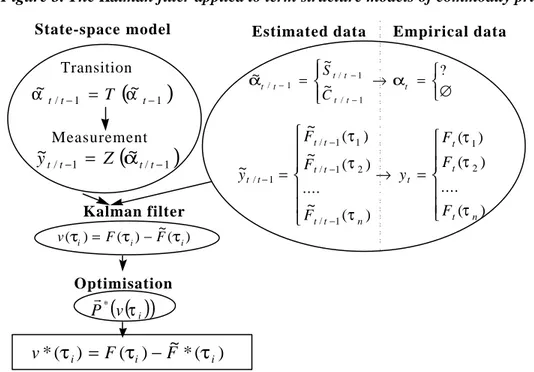
When the Kalman filter is applied to term structure models of commodity prices, the aim is the estimation of the measurement equation’s parameters, in order to obtain estimated
futures prices for different maturities F~
( )
τi , and to compare them with empirical futures prices( )
iFτ , as is shown in figure 3. The closest the firsts are with the seconds, the best is the model. So the way we use the Kalman filter is not perfectly straightforward, because the reconstitution of temporal series for non-observable data is not the most important objective, and because the Kalman filter is always associated with an estimation method for the parameters. But there is still a need for the values of the non-observable data to obtain the observable ones which, in that case, are the futures prices for different maturities. And the Kalman filter is a very fast mean to get them.
Figure 3. The Kalman filter applied to term structure models of commodity prices
(
/ 1)
1 /~
~
− −=
t t t tZ
y
α
Transition MeasurementEstimated data Empirical data
∅ = → = − − − ? ~ ~ ~ 1 / 1 / 1 / t t t t t t t C S α α State-space model Kalman filter = → = − − − − ) ( .... ) ( ) ( ) ( ~ .... ) ( ~ ) ( ~ ~ 2 1 1 / 2 1 / 1 1 / 1 / n t t t t n t t t t t t t t F F F y F F F y τ τ τ τ τ τ
(
1)
1 / ~ ~ − − = t t t T α α ) ( ~ ) ( ) ( i F i F i v τ = τ − τ Optimisation( )
(
v i)
Pr* τ)
(
*
~
)
(
)
(
*
iF
iF
iv
τ
=
τ
−
τ
In the case of term structure models of commodity prices, the non observable data are, most of the time, the spot price S and the convenience yield C. The later can be briefly defined as the comfort associated with the possession of physical stocks. There are usually no empirical data for these two variables, because there are most of the time no reliable time series for the spot price, and the convenience yield is not a traded asset.
The estimation of term structure models is not straightforward, because the analysis relies on two dimensions in time : the first dimension is the estimation period, between the 1st of September, 2000 and the 15th of August, 2002 for example ; the second dimension is represented by the maturities of the futures contracts, for example the first, the third, the sixth and the ninth months of delivery.
The measure of the model’s performances must take into account these two dimensions. One way to appreciate these performances is to compute the difference between F~ and F for different maturities, at one specific observation date, as is illustrated in figure 4. Here is appreciated the model’s ability, at one specific date, to represent the term structure of commodity prices. In the example represented on the figure 4, the innovation for the shorter
maturity τi is smaller than the innovation for the longer maturity τn and the estimated futures
prices, for all the maturity, present a positive bias : they are always superior than the empirical data.
Figure 4. The estimation for different maturities at one specific date
F( t, Ti ) = F (ττi ) Maturity F(τi )
τ
i ) ( ~ i F ττ
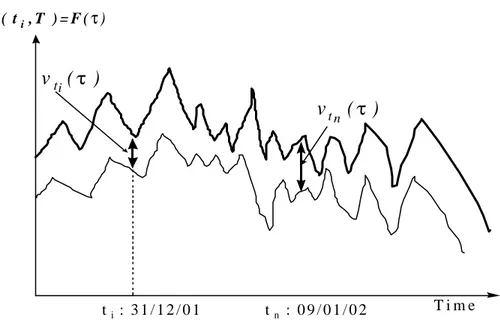
n v(τi ) v(τn )The second way to appreciate the model’s performances is to analyze the estimation’s error for one specific maturity τi and for the whole estimation period, as is show in figure 5.
This time, the figure illustrates a negative bias in the estimation for the maturity τi : for each
date of the estimation sample, the estimated futures prices are always below the empirical data.
Figure 5. The estimation for one specific maturity
T i m e F ( ti , T ) = F (τ) ti : 3 1 / 1 2 / 0 1 tn : 0 9 / 0 1 / 0 2
v
ti(
τ
)
v
t n(
τ
)
2.2. Schwartz’s modelThe Schwartz model (1997) is one of the most famous term structure models of commodity prices. It presents three characteristics. First, its performances are good. Second, it
has an analytical solution, which simplifies the application of the Kalman filter. Third, it allows for the use of a simple filter.
The Schwartz’s model supposes that two states variables, namely the spot price S and the convenience yield C, can explain the behavior of the futures prices F. The dynamic of these state variables is the following :
(
)
[
]
+
−
=
+
−
=
C C S Sdz
dt
C
k
dC
Sdz
Sdt
C
dS
σ
α
σ
µ
)
(
with :E
[
dz
S×
dz
C]
=
ρ
dt
κ, σS, σC >0where : - µ is the immediate return expected for the spot price S, -
σ
S is the spot price’s volatility,- dzS is the increment of the Brownian motion associated with S,
- α is the long run mean of the convenience yield C,
- κ represents the convergence of the convenience yield towards α, -
σ
C is the convenience yield’s volatility,- dzC is the increment of the Brownian motion associated with C.
- ρ is the correlation between the two Brownian motions associated with S and C, The model’s solution expresses the relationship at t between an observable futures price F for a delivery in T, and the state variables. This solution is :
( )
+ − − × = − τ κ κτ B e t C t S T t C S F( , , , ) () exp ( )1 with :( )
− × − + + − × + × − + − = − 2− 2 3 2 2 2 2 1 1 4 2 κ κ σ ρ σ σ κ α κ σ τ κ ρ σ σ κ σ α τ r e κτ eκτ B C C S C C S C ) ) ,(
λ κ)
α α)= − /where : - r is the risk free interest rate7,
- λ is the risk premium associated with the convenience yield, - τ = T - t is the maturity of the futures contract.
To appreciate the model’s performances, there is first of all a need for the optimal values of all the parameters (µ,
σ
S, α, κ,σ
C, and ρ ). These optimal parameters will then be employed to compute the estimated futures prices for different maturities, and to compare them with empirical data.2.3. Applying the simple filter to the Schwartz’s model
The simple filter is suited for linear models. To apply it, the solution of the Schwartz’s model can be easily expressed on a linear form, as follows :
(
)
( )
( )
τ κ κτ B e t C t S T t C S F = − × − + − 1 ) ( ) ( ln ) , , , ( lnConsidering the relationship G = ln(S), we also have :
(
)
[
]
+ − = + − − = C C S S S dz dt C k dC dz dt C dG σ α σ σ µ ) 2 1 ( 2Then, to employ a Kalman filter, the model must be expressed on its state-space form. A state-space model is characterized by its transition and its measurement equation.
The transition equation is the expression, in discrete time, of the state variables dynamic. Retaining the same notations as before, this equation is :
t t t t t t t R C G T c C G η + × + = − − − − 1 1 1 / 1 / ~ ~ ~ ~ , t = 1, ... NT where : -
∆
∆
−
=
t
t
c
Sκα
σ
µ
22
1
is a (2×1) vector, and ∆t is the period separating 2 observation dates
-
∆
−
∆
−
=
t
t
T
κ
1
0
1
is a (2 × 2) matrix, - R is an identity matrix, (2 × 2), - ηt are non correlated errors, with :E[ηt] = 0, and
∆
∆
∆
∆
=
=
t
t
t
t
Var
Q
C C S C S S t 2 2]
[
σ
σ
ρσ
σ
ρσ
σ
η
The measurement equation is issued from the solution of the model :
t t t t t t t C G Z d y +ε × + = − − − 1 / 1 / 1 / ~ ~ ~ , t = 1, ... NT where :
- ~yt/t−1=
[
ln( )
F~( )
τi]
is the ith line of the ~yt/t−1 vector for the estimated observable variables, with i= 1,..,N. N is the number of maturities which where retained for the estimation. - d = [B(τi)] is the ith
line of the d vector, with i = 1,..., N
-
−
−
=
−κ
κτie
Z
1
,
1
is the ith line of the Z matrix, which is (N×2), with i = 1,...,N - εt is a white noise’s vector, (N×1), with no serial correlation :E[εt] = 0 and H = Var[εt]. H is (N × N)
2.4. Applying the extended filter to the Schwartz’s model
From a practical point of view, passing from the simple to the extended filter implies that the system’s matrices Z, T and R are replaced with non linear functions, depending on the
state variables. And to employ the extended Kalman filter, there is no need to express the Schwartz’s solution on a linear form.
The transition equation is directly issued from the dynamic of the state variables. In discrete time, keeping the same notations as before, this dynamic becomes :
t t t t t t t t t T S C R S C C S η ) ~ , ~ ( ) ~ , ~ ( ~ ~ 1 1 1 1 1 / 1 / − − − − − − = + where : - − − 1 / 1 / ~ ~ t t t t C S
is the state vector, (2× 1),
- T(S~t−1,C~t−1) is a (2×1) vector :
(
)
(
)
(
)
∆ − + ∆ ∆ − ∆ + = − − − − − t C t t C t µ S C S T t t t t t κ κα ~ 1 ~ 1 ~ ~ , ~ 1 1 1 1 1 - R(S~t−1,C~t−1)is a (2× 2) matrix :(
)
= − − − 1 0 0 ~ ~ , ~ 1 1 1 t t t S C S R - Q is a (2 × 2) matrix :( )
=
2 2 C C S C S S tVar
σ
σ
ρσ
σ
ρσ
σ
η
The measurement equation becomes :
(
t t t t)
t t t Z S C y/ −1= ~/ −1,~/ −1 +ε ~ where :- ~yt/t−1=F~
( )
τi is the ith line of the ~yt/t−1 vector for the estimated observable variables, with i= 1,..,N.- Z
(
S~t/t−1,C~t/t−1)
is a (N×2) matrix. The ith line of this matrix is the following (i= 1,..,N) :(
S~t/t 1,C~t/t 1)
[
S~t/t 1 exp(
HiC~t/t 1 B( i))
]
Z − − = − × − − + τ with : κ κτi e Hi − − =1 − × − + + − × + × − + − = − 2− 2 3 2 2 2 2 1 1 4 2 ) ( κ κ σ ρ σ σ κ α κ σ τ κ ρ σ σ κ σ α τ r e κτi eκτi B C C S C i C S C i ) ) κ λ α α)= − /- εt is a white noise’s vector, (N×1), with no serial correlation:
E[εt] = 0 and H = Var[εt]. H is (N × N)
Lastly, the derivatives of the functions T and R conditionally to the state variables, respectively
Tˆ
andRˆ
, are the following :- Tˆ is a (2×2) matrix :
(
)
(
)
∆ − ∆ − ∆ − ∆ + = − − − − t t S t C t µ C S T t t t t κ 1 0 ~ ~ 1 ~ , ~ 1 1 1 1 )-
Zˆ
is a (2×N) matrix. The ith line of this matrix is the following, with i = 1,...N :(
)
[
(
~ ( ))
(
~ ( ))
]
1 1 1 1 ~ , ~ ˆ i t i HiCt B i i B C H t t C e H e S Z − − = − −+ τ − × − −+ τ where : κ κτi e Hi − − =1 − × − + + × − + × − + − = 22 2 1 −32 2 1 −2 4 2 ) ( κ κ σ ρ σ σ κ α κ σ τ κ ρ σ σ κ σ α τ r e κτi e κτi B C C S C i C S C i ) ) κ λ α α)= − /
The extended Kalman filter is based on the linearization of the function linking the observable variables to the non-observable. Therefore, an approximation is made in this filter which is absent of the simple one.
2.5. Practical difficulties associated with the empirical study
To perform the empirical study, some difficulties must be overcome. First, there are choices to make when the iterative process is started. Second, if the model has been expressed in logarithm for the simple Kalman filter, some precautions must be taken when the performances are appreciated. Third the stability of the iteration process and the model’s performances are extremely sensitive to the covariance matrix H.
2.5.1. Starting the iterative process
To start the iterative process, there is a need for the initial values of the non-observable variables and for their covariance matrix. Indeed, to proceed with the iteration’s prediction step at date 1, the values of the state variables and of the covariance matrix at date 0 must be known. Because the states variables are non observable, an approximation must be chosen.
In the case of term structure models of commodity prices, the non-observable state variables are most of the time, the spot price and the convenience yield. The nearest futures price is generally retained as the spot price S, and the convenience yield C is computed with the solution of a simple term structure model, more precisely the Brennan and Schwartz’s model (1985). This solution requires the use of two observed futures prices, for delivery in T1 and in
T2 :
(
)
(
)
2 1 2 1) ln ( , , ) , , ( ln T T T t S F T t S F r c − − − =where T1 is the nearest delivery, and T2 is just after.
The covariance matrix associated with the state variables must also be initialized. We choose a diagonal matrix, with the spot price’s variance and the convenience yield’s variance on the diagonal.
Once the approximation’s method has been chosen, we had to decide which value to retain for the state variables and the covariance matrix. We choose the first value of the estimation period for the non-observable variables, and we computed the variances with the first 30 data of the estimation period.
To start the iterative process for the optimization, there is also a need for the parameters initial values. If the iteration process appears to be unstable, constraints can be added on the parameters.
2.5.2. Measuring the performances
When the solution of the model is expressed on its logarithmic form, some precautions must be taken when the model’s performances are measured. Indeed in that case, the innovations are computed with the logarithm of the futures prices. Therefore there is a difficulty when the estimated and empirical data are rebuilt. The relationship linking the logarithm of the estimations
~
y
t/t−1 with the logarithm of the observation yt is actually the following :R
y
y
t=
~
t/t−1+
σ
where σ is the standard error of the innovations and R is a gaussian residue. To be perfectly correct, when the logarithm of the estimations is used to obtain the estimations themselves, the relationship between yt and
~
y
t/t−1 becomes :R y y
e
e
e
t=
~t/t−1×
σThe expectation of the observation’s exponential is then8 :
[ ] [ ]
~ 2 2 1 / σe
e
E
e
E
yt=
ytt−×
When the simple Kalman filter is applied to a model like the Schwartz’s model, when the estimated futures prices are compared with the empirical data, a corrective term should be added to the estimations exponential. The trouble is, this correction is delicate, because the innovations variance is modified as soon as the parameters change.
2.5.3. Stabilizing the iteration process
An other important choice must be made before initiating the Kalman’s iteration process. This choice concerns the estimation of the covariance’s matrix associated with the errors introduced in the measurement equation. This system’s matrix H is very important for the iteration’s stability, because it is added, during the innovation phase, to the innovation covariance’s matrix. In the simple Kalman filter, the relationship between the innovation’s matrix Ft and the system’s matrix H is actually the following :
H Z ZP Ft = t/t−1 '+
where Pt/t-1 is the covariance matrix associated with the non-observable variables α~t, and Z is an
other system’s matrix, included in the measurement equation.
During the next phase of the iteration process, the inverse of the innovation’s matrix is used for the updating of the non-observable variables and their covariance matrix :
(
)
− = + = − − − − − − 1 / 1 1 / 1 ' 1 / 1 / ˆ ' ˆ ˆ ~ ~ t t t t t t t t t t t t t t t t P Z F Z P I P v F Z P α αTherefore, the updating of the non observable variable are strongly affected by the matrix H. And if the terms of this matrix are too high, the iteration can become unstable.
Most of the time, the easiest way to estimate this matrix is to compute the variances and the covariances of the estimation’s database. This method was retained to measure the model’s performances presented in the paragraph 3.3. But it is important to know how much the
8 1 / ~ − t t y
empirical results are affected by this choice. To show it, some simulations are presented in the paragraph 3.4.
S
ECTION3. C
OMPARISON BETWEEN THE TWO FILTERSThe comparison between the performances of the Schwartz’s model measured with the two filters allows appreciating the influence of the linearization on the results. In this section, the empirical data are first of all presented. Then the performance criteria are exposed. Finally, the results are delivered and commented.
3.1. The empirical data
The data used for the empirical study are daily crude oil prices for the settlement of the Nymex’s WTI futures contracts, between the 25th of September, 1995, to the 14th of January, 2002. They have been arranged such as the first futures price’s maturity τ1 is actually the one
month’s maturity, and such as the second futures price’s corresponds to the two months maturity τ2, ... Keeping the first observation of each group of five, this daily data were
transformed into weekly data. For the parameter estimation, and for the measure of the model’s performances, four series of futures prices9 were retained, corresponding to the one, the three, the six and the nine months maturities.
The interest rates are T-bill rates for a three months maturity. Because interest rates are supposed to be constant in the model, we used the mean of all the observations between 1995 and 2002.
3.2. The performances criteria
To measure the model’s performances, two criteria were retained : the mean pricing errors and the root mean squared errors.
The mean pricing errors (MPE) are defined in the following way :
( ) ( )
(
)
∑
= − = N n n F n F N MPE 1 , , ~ 1 τ τwhere N is the number of observations, F~
( )
n,τ is the estimated futures price for maturity τ at the date n, and F( )
n,τ is the observed futures price. The mean pricing error is expressed in US dollar. It measures the estimation’s bias for one given maturity. If the estimation is good, the mean pricing error must be very close to zero.Retaining the same notations, the root mean squared error (RMSE), expressed in US dollar, is defined in the following way, for one given maturity τ :
9 This means that N = 4 in the case we study.
( ) ( )
(
)
∑
= − = N n n F n F N RMSE 1 2 , , ~ 1 τ τThe RMSE is an empirical variance. It measures the estimation stability. This second criteria is considered as the most representative, because prices errors can offset themselves and the mean pricing error can be low even if there are strong deviations.
3.3. The empirical results
The estimation period used to obtain the parameters are the following : from the 25th of September, 1995, to the 11th of May, 1998 and from the 18th of May, 1998, to the 15th of October, 2001. These period have different lengths (respectively 31,5 and 53 months) because we wanted to measure the influence of the available information’s volume on the model’s performances. First, the optimal parameters obtained with the two filters are compared. Then the model’s ability to represent the prices curve and their dynamic is appreciated, on the learning database and on an expanded one. Finally, the sensitivity of the results to the error covariance matrix is presented.
3.3.1. Optimal parameters
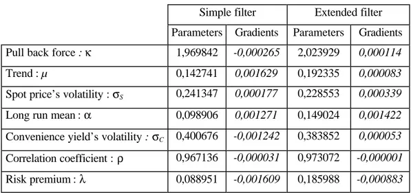
The optimal parameters were estimated on two study periods with the simple and the extended filters. Their values are not the same10, as is illustrated by the tables 1 and 2.
Table 1. Optimal parameters, 1995-199811
Simple filter Extended filter Parameters Gradients Parameters Gradients Pull back force : κ 1,969842 -0,000265 2,023929 0,000114
Trend : µ 0,142741 0,001629 0,192335 0,000083
Spot price’s volatility : σS 0,241347 0,000177 0,228553 0,000339
Long run mean : α 0,098906 0,001271 0,149024 0,001422
Convenience yield’s volatility : σC 0,400676 -0,001242 0,383852 0,000053
Correlation coefficient : ρ 0,967136 -0,000031 0,973072 -0,000001 Risk premium : λ 0,088951 -0,001609 0,185988 -0,000883
During this first period, the optimal parameters obtained with the extended filter are most of the time higher than the ones associated with the simple filter. The principal differences concern the risk premium λ (110%), and the convenience yield’s long run mean α (50%). This
10 In the whole empirical study, optimizations have been made with a precision of 1e
-5 on the gradients.
11 For the two filters, and for the two periods, the parameters values retained to initiate the optimization are the
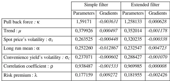
phenomenon does not reproduce itself during 1998-2001, as is shown in table 2 : in that case, the differences between the two parameters series are lower, and the most important deviations are on the convenience yield’s volatility σC (26%) and the spot price’s volatility σS (23%).
Table 2. Optimal parameters, 1998-2001
Simple filter Extended filter Parameters Gradients Parameters Gradients Pull back force : κ 1,59171 -0,003631 1,258133 0,000628
Trend : µ 0,379926 0,000497 0,352014 -0,001178
Spot price’s volatility : σS 0,263525 -0,000448 0,320235 -0,000338
Long run mean : α 0,252260 -0,012867 0,232547 0,004723 Convenience yield’s volatility : σC 0,237071 -0,000602 0,288427 -0,001070
Correlation coefficient : ρ 0,938487 -0,001533 0,969985 0,000008 Risk premium : λ 0,177159 0,009272 0,181955 -0,002426
The differences between the optimal parameters obtained with the two filters show, first that the linearization has a significant influence12, and second, that the parameters are not the same for different periods. In this study, the trend and the convenience yield’s long run mean are significantly higher for the second period.
3.3.2. The model’s performances
There are two ways to measure a model’s performances. The first uses the mean pricing error and the root mean squared errors to see how the model’s can duplicate the form of the term structure of futures prices. The second refers to graphics to show how the model reproduces the dynamic of the price curve.
• The ability to reproduce the form of the term structure of futures prices
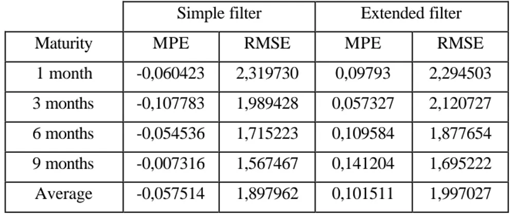
The first important conclusion of the study is that the model is able to reproduce the prices curve quite precisely, as in shown in the tables 3 and 4. For a nine-month maturity, the mean pricing error is around USD 0,12 per barrel ! And the RMSE is quite low, especially for the shorter period. The second conclusion is that if the RMSE is the relevant criteria, then the simple filter is always more precise than the extended one. This is true for the two periods, for all the maturities13. These measure also always decreases with maturity, which is consistent with Schwartz’s results on others periods. Nevertheless, Schwartz has worked with longer
12 Nevertheless, the parameters have the same order size that the one Schwartz obtained in 1997 on the crude oil market, on different periods.
13 The MPE and the RMSE presented here can not directly be compared with the one Schwartz proposed in 1997, because this author has made the calculus with the logarithm of the futures prices.
maturities, and shown that the root mean squared error increases again for deliveries after 15 months.
Table 3. The model’s performances with the simple and the extended filters, 1995-1998 Simple filter Extended filter
Maturity MPE RMSE MPE RMSE
1 month -0,063 1,2769 0,0775 1,3972 3 months 0,1064 1,1804 0,2145 1,3011 6 months 0,1453 1,0142 0,2235 1,0861 9 months 0,1419 0,8468 0,2029 0,8812 Average 0,0827 1,0796 0,1796 1,1664 Unit : USD/b.
The third conclusion is that the results obtained with the mean pricing errors are consistent with the previous one. The errors are always lower for the simple filter. Nevertheless, on the two periods, except for one maturity, the mean pricing errors have a general tendency to increase with the maturity. From 1995 to 1998, and for the two filters, they present a low positive bias, which turns into a negative one for the simple filter, during 1998-2001.
Table 4. The model’s performances with the simple and the extended filters, 1998-2001 Simple filter Extended filter
Maturity MPE RMSE MPE RMSE
1 month -0,060423 2,319730 0,09793 2,294503 3 months -0,107783 1,989428 0,057327 2,120727 6 months -0,054536 1,715223 0,109584 1,877654 9 months -0,007316 1,567467 0,141204 1,695222 Average -0,057514 1,897962 0,101511 1,997027 Unit : USD/b.
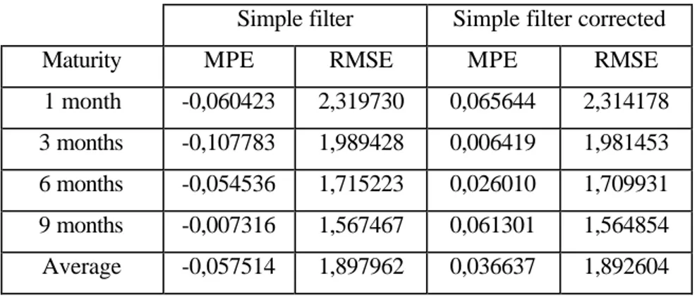
To be perfectly rigorous, the model’s performances associated with the simple Kalman filter should be corrected when, as is the case here, the logarithm of the estimations is used to obtain the estimations themselves (see 2.5.2.). The correction improves a little the performances, as is shown in table 5 : the root mean squared errors and the mean pricing errors diminish a bit for almost all the maturities.
Table 5. The comparison between the model’s performances associated with the simple filter, when there are or there are no corrections for the logarithm, 1998-2001
Simple filter Simple filter corrected
Maturity MPE RMSE MPE RMSE
1 month -0,060423 2,319730 0,065644 2,314178 3 months -0,107783 1,989428 0,006419 1,981453 6 months -0,054536 1,715223 0,026010 1,709931 9 months -0,007316 1,567467 0,061301 1,564854 Average -0,057514 1,897962 0,036637 1,892604 Unit : USD/b.
Finally, the innovation range diminishes with the futures contracts maturity, for the two periods. The figure 6 illustrates the innovation behavior for the one-month’s maturity. It shows that they tend to return to zero, for the two periods and for the two filters. This is a good result, because this is what they are supposed to do in the Kalman filters. Nevertheless, as the figure illustrates it, even if the mean pricing errors are low for the two filters, the pricing errors, at certain specific dates, can be rather important. The maximum innovation in absolute value, for the extended filter, is USD 3,44 during 1995-1998, which represents 17% of the mean futures price for the one-month maturity. For the simple filter, it is USD 3,21 or 15;86% of the mean futures price. For that period and for that maturity, the average of the innovations represents 0,4% of the mean futures price for a one-month maturity for the extended filter, and 0,31% for the simple filter.
Figure 6. Innovations, 1998-2001 -7 -6 -5 -4 -3 -2 -1 0 1 2 3 4 5 6 7 18/05/9818/07/9818/09/9818/11/9818/01/9918/03/9918/05/9918/07/9918/09/9918/11/9918/01/0018/03/0018/05/0018/07/0018/09/0018/11/0018/01/0118/03/0118/05/0118/07/0118/09/01 ($/b)
The maximum innovation increases a lot during the second period. In absolute value, during 1998-2001, it reaches USD 6 for the extended filter, which represents 25% of the mean futures price for a one-month maturity. It is a bit lower for the simple filter : USD 5.
Therefore, as a conclusion, we can say that there is clearly an impact of the linearization introduced in the extended filter : it can be shown on the optimal parameters, on the performances, and on the innovations. Nevertheless, with an extended filter, the model’s ability to represent the prices curve is still good.
• The ability to reproduce the dynamic of the term structure of futures prices
An other way to appreciate a model’s performances is to see if it is able to reproduce the price’s dynamic. This can be shown graphically.
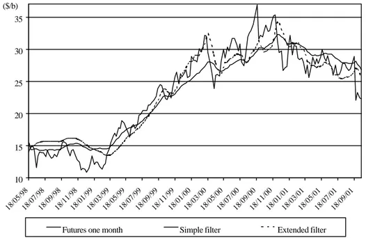
On that point of view, the first important conclusion is that the model is able to reproduce the prices dynamic quite precisely, even if, like in 1998-2001, there are very large fluctuations in the futures prices. The figure 7 shows the results obtained for the one-month’s maturity. During that period, the crude oil prices goes from USD 11 per barrel to USD 37 per barrel ! Even if the Kalman filters are often suspected to be unstable, these results show that they can be used even with extremely volatile data. The graphic also shows that the two filters attenuate the range of price fluctuations. This phenomenon can actually be observed for the two study periods, for every maturities.
Figure 7. Estimated and observed futures prices for the one month maturity, 1998-2001
10 15 20 25 30 35 18/05/9818/07/9818/09/9818/11/9818/01/9918/03/9918/05/9918/07/9918/09/9918/11/9918/01/0018/03/0018/05/0018/07/0018/09/0018/11/0018/01/0118/03/0118/05/0118/07/0118/09/01 ($/b)
Futures one month Simple filter Extended filter
The second important conclusion concerns the ability to reproduce the way price curves evolve with time.
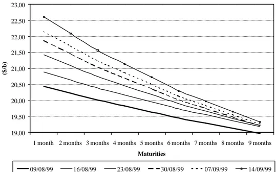
The figure 8 represents six term structures of crude oil prices, for different maturities (one to nine months), observed weekly on the Nymex between the 9th of August and the 14th of September, 1999. During this period, the price curves are always in backwardation, and they are
characterized by the presence of a little bump. Moreover, the intensity of the bakwardation increases and the curve goes higher, as the futures prices for all the maturities rise.
Figure 8. Observed term structures of crude oil prices
19,00 19,50 20,00 20,50 21,00 21,50 22,00 22,50 23,00 23,50 24,00
1 month 2 months 3 months 4 months 5 months 6 months 7 months 8 months 9 months Maturities
($/b)
09/08/99 16/08/99 23/08/99 30/08/99 07/09/99 14/09/99
The figure 9 shows how the model reproduced this evolution. It represents, for the same observations dates, the term structure of crude oil prices which where estimated with a simple Kalman filter. The model is able to replicate correctly not only the displacement towards the heights, but also the slope’s intensification. Finally, despite it is theoretically able to do it, the model doesn’t represent, in this example, the little bump in the curves that was empirically observed
Figure 9. Estimated term structures of crude oil prices
19,00 19,50 20,00 20,50 21,00 21,50 22,00 22,50 23,00
1 month 2 months 3 months 4 months 5 months 6 months 7 months 8 months 9 months
Maturities
($/b)
3.3.3. Expansion of the database
The parameter estimation shows, in 3.3.1, that they are not the same for different periods. Hence two questions arise. Firstly, is it necessary to often recompute the parameters ? Secondly, when does the calculus have to be done ?
To bring a precise answer to these questions, a sensibility’s analysis of the estimated prices to the parameters should be undertaken. But measuring the model’s performances when the database is expanded and the parameters are kept the same as before can make a first step in the comprehension of what happens. This test has been made for two periods of three months, located in the prolongation of the two estimation’s periods : from the 18th of May to the 17th of August 1998 and from the 21st of October 2001 to the 14th of January, 2002.
One important conclusion issued from these tests is that the model’s performance decrease strongly when the database is expanded. The root mean squared errors and the mean pricing errors rise dramatically for the two periods. This phenomenon is particularly strong when the futures prices are volatile, during 2001-2002, and it will probably be even more pronounced as the database expansion’s length increase. Therefore there is a strong incentive to recompute the optimal parameters each time the model is used. This is not especially an important drawback, at least when there is an analytical solution for the model, because then the estimation’s process is very fast.
The differences in the performances we observe with the two filters are inverted when the optimal parameters of a given period are used to estimate futures prices on a period, which is situated after the learning period. The model is then most of the time more precise with the extended filter, and we observed this phenomenon for the two periods, as the tables 6 and 7 illustrate it.
Table 6. The model’s performances with an extrapolation on a three months period, in 1998 Simple filter Extended filter
Maturity MPE RMSE MPE RMSE
1 month 2,0138 2,2012 1,7392 1,8834
3 months 1,3296 1,3749 1,2448 1,3084
6 months 0,6512 0,755 0,7563 0,8691
9 months 0,2710 0,5442 0,4883 0,6540
Average 1,0664 1,2188 1,0572 1,1787
The results we obtain with an extrapolation on three months are nevertheless more in the favor of the extended filter in 1995 than in 1998. In the first case, what ever the maturity is considered, the mean pricing errors and the root mean squared errors are much lower with the extended filter. For the second period, the extended filter’s advantage disappears when the maturity reaches the sixth month, although, in average, it is still more precise.
Table 7. The model’s performances with an extrapolation on a 3 months period, in 2001-2002 Simple filter Extended filter
Maturity MPE RMSE MPE RMSE
1 month -0,710678 3,371702 -3,243584 3,837790 3 months -0,379108 2,972144 -2,920091 3,408698 6 months 0,155104 2,500216 -2,247877 2,649836 9 months 0,385290 2,164323 -1,767425 2,123121 Average -0,137348 2,750296 -2,544744 3,004861 3.4. Simulations
The last results presented in this article are simulations. They show how the model’s performances are affected by the choice of the system’s matrix H. This matrix represents the errors in the measurement equation and the way it is estimated has a strong influence on the empirical results.
Most of the time, the terms of this matrix corresponds to the variances and the covariances of the estimation database, namely, in the case studied here, the variances and covariance between futures prices for different maturities. But one must know that the results obtained with the Kalman filter can be more precise if these terms are (artificially) lowered, as is shown in table 8. This table exposes the different results obtained during 1998-2001 with the extended Kalman filter. This period is especially interesting because the data fluctuate strongly The performances are achieved, first with the matrix based on the observations, then with artificially lowered matrices.
Table 8. Simulations with different system’s matrix H
Observations 1 month 3 months 6 months 9 months Average
MPE 0,0979 0,0573 0,1096 0,1412 0,1015
RMSE 2,2945 2,1207 1,8777 1,6952 1,9970
Simulation 1 1 month 3 months 6 months 9 months Average
MPE 0,0013 0,0935 0,1501 1,6506 0,4739
RMSE 1,8356 1,5405 1,2478 2,6602 1,8210
Simulation 2 1 month 3 months 6 months 9 months Average
MPE 0,0073 0,0152 0,0612 0,0137 0,0244
RMSE 1,4759 1,1686 0,9386 0,8317 1,1037
Simulation 3 1 month 3 months 6 months 9 months Average
MPE 0,0035 -0,0003 0,0383 0,0005 0,0105
RMSE 1,3812 1,0950 0,8647 0,7499 1,0227
Simulation 4 1 month 3 months 6 months 9 months Average
MPE 0,0131 0,0067 0,0415 0,0075 0,0172
The simulations 1 to 4 correspond respectively to the model’s performances obtained by multiplying the system’s matrix H by (1/2), (1/16), (1/160), and (1/1600). As the matrix is lowered, the model’s performances improve strongly : from the initial performances to the fourth simulation, the root mean squared error is almost divided by two. The comparison between the third and the fourth simulation also illustrates the fact that there is a limit to the performance amelioration. The figure 10 portrays the main results of these simulations.
Figure 10. One month’s futures prices observed/estimated, 1998 - 2001
10,00 15,00 20,00 25,00 30,00 35,00 18/05/98 18/07/98 18/09/98 18/11/98 18/01/99 18/03/99 18/05/99 18/07/99 18/09/99 18/11/99 18/01/00 18/03/00 18/05/00 18/07/00 18/09/00 18/11/00 18/01/01 18/03/01 18/05/01 18/07/01 18/09/01 ($/b)
Observed futures prices for a one month's maturity
Estimated futures prices for a one month's maturity with a matrix H corresponding to the observations. Estimated futures prices for a one month maturity and an artificially lowered matrix (Simulation 4)
S
ECTION4. C
ONCLUSIONThe Kalman filters are powerful tools, which can be employed for model’s estimation in many areas in finance. They are especially well suited for finance because they are fast even if they have to deal with a large amount of information and because they allow for unobservable variables. Moreover, they can be used for linear as well as non-linear models, even if there is no analytical solution for the models.
The main conclusions of this article are the following. First, the extended Kalman filter introduces an approximation, which is due to the model’s linearization. This approximation has clearly an influence on the model’s performances: the extended filter leads generally to less precise estimations than the simple one. Nevertheless, the difference between the two filters is quite low and the extended filter is still acceptable. The second conclusion is that the estimation results are sensible to the system’s matrix containing the errors of the measurement equation and that this matrix can be used to obtain more precise results on the estimation base. The third important conclusion is that at least for the term structure models of commodity prices, the parameters are not constant in time and there is a need to recompute them very often. This can become a problem if the model has no analytical solution, because of the computing time.
Lastly, the approximation made in the extended Kalman filter is not a real problem until the model becomes really non-linear. In that case, some other methods may be used, like the one Küchner (1968) proposed. The study of this method, also well suited for non-linear models, constitute the natural prolongation of this work.
REFERENCES
B. D. O. ANDERSON AND J. B. MOORE., 1979, Optimal filtering, Englewood Cliffs, Prentice
Hall.
Simon H. BABBS and K. Ben NOWMAN, 1999, “Kalman Filtering of Generalized Vasicek Term Structure Models”, Journal of Financial and Quantitative Analysis, vol 34, n°1, pp 115-130, March.
Michael J.BRENNAN and Eduardo S.SCHWARTZ, 1985 :« Evaluating Natural Ressource Investments », The
Journal of Business, vol. 58, n°2.
A. C. HARVEY, 1989, Forecasting, structural time series models and the Kalman filter, Cambridge University Press.
D. LAUTIER, 2000, La structure par terme des prix des commodités : analyse théorique et applications au marché pétrolier, Thèse de doctorat, Université Paris IX, 421 p.
George G. PENNACCHI, 1991, “Identifying the Dynamics of Real Interest Rates and Inflation : Evidence Using Survey Data”, The Review of Financial Studies, vol 4, n°1, pp 53-86.
W. H. PRESS, B.P.FLANNERY, S.A. TEUKOLSKY, W.T. VETTERLING, 1992, Numerical Recipes in C : The Art
of Scientific Computing, 2d Edition, Cambridge University Press.
Thierry RONCALLI, 1995, Introduction à la programmation sous Gauss, Ritme informatique.
Suresh M. SUNDARESAN, 2000, “Continuous-Time Methods in Finance : A Review and an Assessment”, Journal of Finance, vol LV, n°4, pp 1569-1621, August.
Eduardo S. SCHWARTZ, 1997 : « The Stochastic Behavior of Commodity Prices : Implications for Valuation and Hedging », The Journal of Finance, vol. LII, n°3, July.