O
pen
A
rchive
T
OULOUSE
A
rchive
O
uverte (
OATAO
)
OATAO is an open access repository that collects the work of Toulouse researchers and
makes it freely available over the web where possible.
This is an author-deposited version published in :
http://oatao.univ-toulouse.fr/
Eprints ID : 16938
The contribution was presented at SEG 2015 :
https://seg.org/web/seg-new-orleans-2015/
To cite this version :
Amestoy, Patrick and Brossier, Romain and Buttari,
Alfredo and L'Excellent, Jean-Yves and Mary, Théo and Métivier, Ludovic
and Miniussi, Alain and Operto, Stéphane and Virieux, Jean and Weisbecker,
Clément 3D frequency-domain seismic modeling with a Parallel BLR
multifrontal direct solver. (2015) In: Society of Exploration Geophysicists
annual meeting (SEG 2015), 18 October 2015 - 23 October 2015
(New-Orleans, United States).
Any correspondence concerning this service should be sent to the repository
administrator:
[email protected]
3D frequency-domain seismic modeling with a Parallel BLR multifrontal direct solver
P. Amestoy∗, R. Brossier∗∗, A. Buttari‡, J.-Y. L’Excellent§, T. Mary†,††, L. M´etivier∗∗, A. Miniussi¶, S. Operto¶, J. Virieuxk, C. Weisbecker∗
∗INPT-IRIT; ‡CNRS-IRIT; †UPS-IRIT; §INRIA-LIP; ¶Geoazur-CNRS-UNSA; kISTERRE-UJF; ∗∗
ISTERRE-LJK-CNRS;††Speaker
SUMMARY
Three-dimensional frequency-domain full waveform inversion (FWI) of fixed-spread data can be efficiently performed in the visco-acoustic approximation when seismic modeling is based on a sparse direct solver. We present a parallel algebraic Block Low-Rank (BLR) multifrontal solver which provides an ap-proximate solution of the time-harmonic wave equation with a reduced operation count, memory demand, and volume of communication relative to the full-rank solver. We analyze the parallel efficiency and the accuracy of the solver with a realis-tic FWI case study from the Valhall oil field.
INTRODUCTION
Seismic modeling and full waveform inversion (FWI) can be performed either in the time domain or in the frequency main (e.g., Virieux and Operto, 2009). In the frequency do-main, seismic modeling consists of solving an elliptic boundary-value problem, which can be recast in matrix form as a system of linear equations where the solution (i.e., the monochromatic wavefield) is related to the right-hand side (i.e., the seismic source) through a sparse impedance matrix, whose coefficients depend on frequency and subsurface properties (e.g., Marfurt, 1984). One distinct advantage of the frequency domain is to allow for a straightforward implementation of attenuation in seismic modeling (e.g., Toks¨oz and Johnston, 1981). Second, it provides a suitable framework to implement multi-scale FWI by frequency hopping, that is useful to mitigate the nonlin-earity of the inversion (e.g., Pratt, 1999). Third, monochro-matic wavefields can be computed quite efficiently for mul-tiple sources by forward/backward substitutions if the linear system can be solved with a sparse direct solver based on the multifrontal method (Duff and Reid, 1983). However, the LU factorization of the impedance matrix that is performed before the substitution step generates fill-in, which makes this pre-processing step memory demanding. Dedicated finite-difference stencils of local support (Operto et al., 2014) and fill-reducing matrix ordering based on nested dissection (George and Liu, 1981) are commonly used to minimize this fill-in.
This limitation motivates to compute approximate solutions of the linear system by exploiting the low-rank properties of el-liptic partial differential operators (Wang et al., 2011). Several approaches exist to achieve this objective. The Block Low-Rank (BLR) approach (Amestoy et al., 2015b) can be easily and efficiently embedded in a multifrontal solver. In Weis-becker et al. (2013), we presented its potential in a sequential environment using the BLR solver. In this study, we gener-alize the approach to a parallel context and present the
chal-lenges that need to be overcome to preserve the efficiency of the solver on modern distributed-memory machines with mul-ticore processors. In the first part, we review the main fea-tures of the parallel BLR multifrontal solver. Second, seismic modeling in a subsurface model of the Valhall oil field in the 3.5Hz-10Hz frequency band gives quantitative insights on the memory and operation count savings provided by the BLR ap-proach. We also present the parallel performance of the solver. The relevance of the BLR approach to perform FWI of real ocean-bottom cable data recorded in the Valhall oil field is il-lustrated in a companion abstract (Amestoy et al., 2015a).
PARALLEL BLOCK LOW-RANK MULTIFRONTAL METHOD Parallel Multifrontal method
The multifrontal method was first introduced by Duff and Reid (1983). Being a direct method, it computes the solution of a
sparse system Ax= b by means of a factorization of A under
the form A= LU (in the unsymmetric case). This
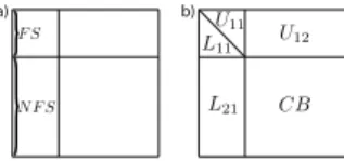
factoriza-tion is achieved through a sequence of partial factorizafactoriza-tions, performed on dense matrices, called fronts. With each front are associated two sets of variables: the fully-summed (FS) variables, whose corresponding rows and columns of L and
U are computed within the current front, and the non
fully-summed (NFS) variables, which receive updates resulting from the elimination of FS variables. At the end of each partial fac-torization, the partial factors[L11L21] and [U11U12] are stored
apart and a Schur complement referred to as a contribution block (CB) is held in a temporary memory area called CB stack, whose maximal size depends on several parameters. As the memory needed to store the factors is incompressible (in full-rank), the CB stack can be viewed as an overhead whose peak has to be minimized. The structure of a front before and after partial factorization is shown in Fig. 1. The
computa-a) b)
Figure 1: A front before (a) and after (b) partial factorization. tional and memory requirements for the complete factorization strongly depend on how the fronts are formed and on the order in which they are processed. Reordering techniques such as nested dissection are used to ensure the efficiency of the pro-cess: a so-called elimination tree (Schreiber, 1982) is created, with a front associated with each of its nodes. Any post-order traversal of this tree gives equivalent properties in terms of fac-tors memory and computational cost.
Seismic modeling with a Block Low-Rank direct solver
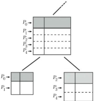
In a parallel environment, two kinds of parallelism, referred to as tree parallelism and node parallelism, are exploited (Fig. 2). In tree parallelism, fronts in different sub-trees are processed by different processes, while in node parallelism, large enough fronts are mapped on several processes: the master process is assigned to process the fully-summed rows and is in charge of organizing computations; the non fully-summed rows are distributed following a one-dimensional row-wise partitioning, so that each slave holds a range of rows.
P2 P3 P4 P0 P1 P0 P1 P2 P3 P4
Figure 2: Illustration of tree and node parallelism. The shaded part of each front represents its fully-summed rows. The fronts are row-wise partitioned in our implementation, but column-wise partitioning is also possible.
Block Low-Rank (BLR) matrices
A flexible, efficient technique can be used to represent fronts with low-rank sub-blocks based on a storage format called Block Low-Rank (BLR, see Amestoy et al. (2015b)). Un-like other formats such as H -matrices (Hackbusch, 1999) and HSS matrices (Xia et al., 2009), the BLR one is based on a flat, non-hierarchical blocking of the matrix which is defined by conveniently clustering the associated unknowns. A BLR representation of a dense matrix F is shown in equation (1) where p sub-blocks have been defined. Sub-blocks eBi jof size
mi× njand numerical rank kεi jare approximated by a low-rank
product Xi jYi jT at accuracy ε, when k ε i j(mi+ nj) ≤ minjis sat-isfied. e F= e B11 · · · Be1p .. . . .. ... e Bp1 · · · Bepp (1)
In order to achieve a satisfactory reduction in both the com-plexity and the memory footprint, sub-blocks have to be cho-sen to be as low-rank as possible (e.g., with exponentially de-caying singular values). This can be achieved by clustering the unknowns in such a way that an admissibility condition (Beben-dorf, 2008) is satisfied. This condition states that a sub-block
e
Bi j, interconnecting variables of i with variables of j, will have
a low rank if variables of i and variables of j are far away in the domain, intuitively, because the associated variables are likely to have a weak interaction. In practice, the sub-graphs induced by the FS variables and the NFS variables are algebraically partitioned with a suitable strategy.
Parallel BLR multifrontal solver
A BLR multifrontal solver consists in approximating the fronts
with BLR matrices. BLR representations of[L11U11], L21, U12
and CB are computed separately. The partial factorization oc-curring at each front of the multifrontal method is then adapted to benefit from the compressions using low-rank products in-stead of full-rank standard ones. An example of a BLR partial factorization algorithm is given in Algorithm 1; many variants can be easily defined, depending on the position of the Com-press operation. For sake of clarity, we present the version with only one process mapped on the front. For fronts with several processes, the Factor task is done on the master, while each slave performs the Solve, Compress and Update tasks on their respective block of rows.
Algorithm 1 Partial dense BLR LU factorization.
1: ◮ Input: a m× m block matrix A of size n; A = [Ai, j]i=1:m, j=1:m; with p the number of blocks to eliminate
2: for k= 1 to p do
3: Factor: Ak,k:m= Lk,kUk,k:m 4: for i= k + 1 to m do
5: Solve (compute L): Ai,k← Ai,kUk,k−1 6: Compress: Ak,i≈ Xk,iYk,iT and Ai,k≈ Xi,kYi,kT 7: end for
8: for i, j = k + 1 to m do
9: Update: Ai, j← Ai, j− Xi,k(Yk,iTXk, j)Yk, jT
10: end for 11: end for
The O(n2) complexity of a standard, full rank solution of a
3D problem (of N unknowns) from the Laplacian operator dis-cretized with a 3D 7-point stencil is reduced to O(n5/3) when using the BLR format (Amestoy et al., 2015b). Although com-pression rates may not be as good as those achieved with hi-erarchical formats, BLR offers a good flexibility thanks to its simple, flat structure. This makes BLR easy to adapt to any multifrontal solver without a complete rethinking of the code. Next, we describe the generalization of the BLR to a parallel environment. The row-wise partitioning imposed by the distri-bution of the front onto several processes constraints the clus-tering of the unknowns. However, in practice, we manage to maintain nearly the same compression rates when the number of processes grows (see Figure 3). Both LU and CB compres-sion can contribute to reducing the volume of communication by a substantial factor and improving the parallel efficiency of the solver. In our implementation, we do not compress the CB. To fully exploit multicore architectures, MPI parallelism is hy-bridized with thread parallelism by multithreading the tasks of Algorithm 1. In full-rank, we exploit multithreaded BLAS kernels. In low-rank, these tasks have a finer granularity and thus a lower efficiency (flop rate). Thus with multithreaded BLAS we are not able to efficiently transform the compres-sion of flops into reduction in time. To overcome this obstacle, Algorithm 1 can be modified to exploit OpenMP-based mul-tithreading instead, which allows for a larger granularity of computations. TheUpdate task at line 9 is applied on a set of independent blocks Ai, j: therefore, the loop at line 8 can
be parallelized. The same applies for theSolve and Compress tasks: the loop at line 4 can also be parallelized using OpenMP.
NUMERICAL EXAMPLE
We perform finite-difference frequency-domain seismic mod-eling (Operto et al., 2014) in a visco-acoustic vertical trans-verse isotropic (VTI) subsurface model of the Valhall oil field (Barkved et al., 2010). This subsurface model, whose
dimen-sions are 16km× 9km × 4.5km, has been developed by
reflec-tion traveltime tomography (courtesy of BP) (Fig. 4a). We per-form seismic modeling for the 5-Hz, 7-Hz and 10-Hz frequen-cies using 12, 16 and 34 computer nodes, respectively. Each node is made of two 10-core IvyBridge E5-2670v2 processor equipped with 64GB of shared memory. We ran 2 MPI pro-cesses per node and 10 threads per MPI process (i.e., 1 thread per core). The full-rank (FR) and the BLR factorizations are performed with single precision arithmetic. A discretization rule of 4-grid points per minimum wavelength leads to a grid interval of 70m, 50m and 35m and a finite-difference grid with perfectly-matched layers of 2.94, 7.17 and 17.27 millions of nodes for the three above-mentioned frequencies. The BLR
solutions are computed for two values of the threshold ε (10−4
and 10−5).
Computational efficiency and accuracy of BLR solver The reduction of the memory demand, operation count and factorization time obtained with the BLR approximation are outlined in Table 1 for the three modeled frequencies. Com-pared to the FR factorization, the time to perform the BLR
factorization (ε= 10−5) is decreased by a factor 1.78, 2.15
and 2.87 for the 5Hz, 7Hz and 10Hz frequencies, respectively. This shows that the computational gain provided by the BLR approximation increases with frequencies (i.e., for larger ma-trices). The same trend is shown for the memory demand of the LU factorization.
The accuracy of the BLR solver is assessed by the differences between the FR solution and the BLR solutions for the 7-Hz
frequency (Fig. 5). This difference is negligible for ε= 10−5
and may be acceptable for FWI applications for ε= 10−4as
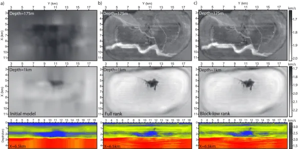
shown hereafter. We apply FWI to a Valhall ocean-bottom ca-ble dataset composed of 2302 hydrophone sensors and 49,954
shots using the FR and BLR solver with ε equal to 10−4and
10−5. Eight frequencies between 3.5Hz and 7Hz are inverted
successively (see Amestoy et al. (2015a) for more details).
The final FWI models obtained with the FR and BLR(ε =
10−4) solvers are very similar. Comparison between the
7-Hz recorded data and the synthetic data computed in the FWI model that has been built with the BLR solver shows an excel-lent agreement (Fig. 5(d-g)).
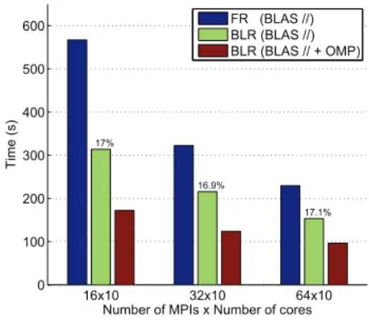
Parallel performance and scalability of BLR solver A parallel performance and strong scalability analysis of the FR and BLR solvers is performed in the Valhall model for the 7Hz frequency using 160, 320 and 640 cores (Fig. 3). The BLR version using multithread BLAS kernels does not fully exploit the compression potential: even though the flops are reduced by a factor 5.9, the time is only reduced by a factor 1.8. With OpenMP-based parallelism, we manage to retrieve a substantial part of this potential, reaching a speedup of 3.3. The scalability of FR solver is good: it obtains a speedup of 1.75 from 160 to 320 cores and of 1.4 from 320 to 640 cores.
The difference between the FR and BLR (with OpenMP) exe-cution times decreases as the number of cores increases. This is due to the fact that the BLR code performs much less Flops and of much smaller granularity; nonetheless the strong scal-ability of the LR factorization is satisfactory and it is reason-able to expect that on problems of larger size, this difference remains considerable even on higher core counts, as evidenced by Table 1. 16x10 32x10 64x10 0 100 200 300 400 500 600 17% 16.9% 17.1%
Number of MPIs x Number of cores
Time (s)
FR (BLAS //) BLR (BLAS //) BLR (BLAS // + OMP)
Figure 3: Scalability of the factorization for the 7Hz frequency.
For BLR, the threshold has been set to ε= 10−4. FR (BLAS
//): Full-rank factorization. BLR (BLAS //): BLR factorization using MKL BLAS kernels for multithreading. BLR (BLAS // + OMP): BLR factorization using OpenMP for multithreading
theUpdate and Compress tasks, MKL BLAS for the rest. The
flop compression rate, provided on top of each bar, remains comparable when the number of processes grows.
CONCLUSION
We have shown the computational efficiency, the accuracy and the parallel performance and scalability of the Block Low-Rank (BLR) algebraic sparse direct solver for frequency-domain seismic modeling. The computational time and memory sav-ings achieved during BLR factorization increase with the size of the computational grid (i.e., frequency). This opens new perspectives to perform efficiently frequency-domain FWI of fixed-spread data on clusters of reasonable size at frequencies up to 15Hz. Other perspectives concern the optimization of the solution step, during which the sparsity of the source vectors can be exploited during the forward substitution step. Acknowledgments
This study was partly funded by the sponsors of the SEIS-COPE consortium. This study was granted access to the HPC resources of SIGAMM and CIMENT computer centers and CINES/IDRIS under the allocation 046091 made by GENCI. We thank BP Norge AS and their Valhall partner Hess Norge AS for allowing access to the Valhall dataset, tomographic models and well-log velocities.
Seismic modeling with a Block Low-Rank direct solver
f # cores Flop count LU Mem LU Time LU
FR BLR FR BLR FR BLR
ε= 10−5 ε= 10−4 ε= 10−5 ε= 10−4 ε= 10−5 ε= 10−4
5Hz 240 6.54E+13 26.5% 23.7% 2530 MB 53.4% 48.9% 80s 45s 40s
7Hz 320 4.05E+14 21.3% 16.9% 6445 MB 45.7% 39.1% 323s 150s 124s
10Hz 680 2.56E+15 20.3% 15.6% 10495 MB 42.5% 35.6% 1117s 389s 338s
Table 1: Statistics of the Full-Rank (FR) and Block Low-Rank (BLR) simulations for ε= 10−5 and ε= 10−4. f : modeled
frequency in Hertz. # cores: number of cores used; we ran 1 MPI process on each socket of 10 cores. Flop count: number of flops during LU factorization. Mem LU: Memory for LU factors in MegaBytes. Time LU: time for LU factorization in seconds. The flops and memory for the low-rank factorization are provided as percentage of those required by the full-rank factorization.
3 4 5 6 7 8 9 10 11 3 5 7 9 11 13 15 17 Y (km) 3 4 5 6 7 8 9 10 11 3 5 7 9 11 13 15 17 Y (km) 3 4 5 6 7 8 9 10 11 3 5 7 9 11 13 15 17 1.7 1.8 1.9 2.0 km/s 3 4 5 6 7 8 9 10 11 3 5 7 9 11 13 15 17 1.7 1.8 1.9 2.0 2.1 2.2 km/s 0 1 2 3 4 3 4 5 6 7 8 9 10 11 12 13 14 15 16 17 18 0 1 2 3 4 3 4 5 6 7 8 9 10 11 12 13 14 15 16 17 18 1.5 2.0 2.5 3.0 km/s
Full rank Block-low rank
3 4 5 6 7 8 9 10 11 X (km) 3 5 7 9 11 13 15 17 Y (km) 3 4 5 6 7 8 9 10 11 X (km) 3 5 7 9 11 13 15 17 0 1 2 3 4 Depth(km) 3 4 5 6 7 8 9 10 11 12 13 14 15 16 17 18 a) b) c) Initial model Depth=175m Depth=1km X=6.5km Depth=175m Depth=175m Depth=1km Depth=1km X=6.5km X=6.5km
Figure 4: Traveltime tomography (a) and 7-Hz FWI (b-c) Valhall models. (b-c) FWI is performed with the FR (b) and the BLR(ε=
10−4) (c) solver. Top panel: horizontal slice across channel system; Middle panel: horizontal slice across a gas cloud; Bottom panel:
vertical section near the periphery of the gas cloud (X=6.5km) (see Sirgue et al. (2009) and Sirgue et al. (2010) for comparison).
3 4 5 6 7 8 9 10 11 X (km) 3 4 5 6 7 8 9 10 11 12 13 14 15 16 17 18 Y (km) a) FR solution -1.5 -1.0 -0.5 0 0.5 1.0 1.5 3 4 5 6 7 8 9 10 11 3 4 5 6 7 8 9 10 11 12 13 14 15 16 17 18 Y (km) b) FR-BLR (H=10-5) -1.5 -1.0 -0.5 0 0.5 1.0 1.5 3 4 5 6 7 8 9 10 11 3 4 5 6 7 8 9 10 11 12 13 14 15 16 17 18 Y (km) c) -1.5 -1.0 -0.5 0 0.5 1.0 1.5 x10 x10 FR-BLR (H=10-4) 3 4 5 6 7 8 9 10 11 X (km) 3 4 5 6 7 8 9 10 11 12 13 14 15 16 17 18 Y (km) d) -1.5 -1.0 -0.5 0 0.5 1.0 1.5 3 4 5 6 7 8 9 10 11 3 4 5 6 7 8 9 10 11 12 13 14 15 16 17 18 Y (km) e) -1.5 -1.0 -0.5 0 0.5 1.0 1.5 3 4 5 6 7 8 9 10 11 3 4 5 6 7 8 9 10 11 12 13 14 15 16 17 18 Y (km) f ) -1.5 -1.0 -0.5 0 0.5 1.0 1.5
Recorded Modeled Difference
BLR (H=10-4) -3 -2 -1 0 1 2 3 4 5 Offset (m ) Amplitude g)
Figure 5: (a) 7-Hz FR solution (real part) computed in the tomography model (Fig. 4a). Pressure wavefield is shown at the shot positions, 5m below the surface. The explosive source, (X,Y)=(15km,5km), is on the sea bottom at 70m depth. (b-c) Differences,
magnified by a factor 10, between FR and BLR solutions (ε= 10−5(b), ε= 10−4(c)). (d) Recorded data (7Hz). (e) Synthetic data
REFERENCES
Amestoy, P., R. Brossier, A. Buttari, J.-Y. L’Excellent, T. Mary, L. M´etivier, A. Miniussi, S. Operto, A. Ribodetti, J. Virieux, and C. Weisbecker, 2015a, Efficient 3D frequency-domain full-waveform inversion of ocean-bottom cable data with sparse block
low-rank direct solver: application to valhall: Presented at the 85thAnnual SEG Meeting (New Orleans).
Amestoy, P. R., C. Ashcraft, O. Boiteau, A. Buttari, J.-Y. L’Excellent, and C. Weisbecker, 2015b, Improving multifrontal methods by means of block low-rank representations: SIAM Journal on Scientific Computing. to appear.
Barkved, O., U. Albertin, P. Heavey, J. Kommedal, J. van Gestel, R. Synnove, H. Pettersen, and C. Kent, 2010, Business impact of full waveform inversion at Valhall: 91 Annual SEG Meeting and Exposition (October 17-22, Denver), Expanded Abstracts, 925–929, Society of Exploration Geophysics.
Bebendorf, M., 2008, Hierarchical matrices: A means to efficiently solve elliptic boundary value problems (lecture notes in com-putational science and engineering): Springer, 1 edition.
Duff, I. S. and J. K. Reid, 1983, The multifrontal solution of indefinite sparse symmetric linear systems: ACM Transactions on Mathematical Software, 9, 302–325.
George, A. and J. W. Liu, 1981, Computer solution of large sparse positive definite systems: Prentice-Hall, Inc.
Hackbusch, W., 1999, A sparse matrix arithmetic based on H -matrices. Part I: Introduction to H -matrices: Computing, 62, 89–108.
Marfurt, K., 1984, Accuracy of finite-difference anf finite-element modeling of the scalar and elastic wave equations: Geophysics, 49, 533–549.
Operto, S., R. Brossier, L. Combe, L. M´etivier, A. Ribodetti, and J. Virieux, 2014, Computationally-efficient three-dimensional visco-acoustic finite-difference frequency-domain seismic modeling in vertical transversely isotropic media with sparse direct solver: Geophysics, 79(5), T257–T275.
Pratt, R. G., 1999, Seismic waveform inversion in the frequency domain, part I : theory and verification in a physic scale model: Geophysics, 64, 888–901.
Schreiber, R., 1982, A new implementation of sparse Gaussian elimination: ACM Transactions on Mathematical Software, 8, 256–276.
Sirgue, L., O. I. Barkved, J. Dellinger, J. Etgen, U. Albertin, and J. H. Kommedal, 2010, Full waveform inversion: the next leap forward in imaging at Valhall: First Break, 28, 65–70.
Sirgue, L., O. I. Barkved, J. P. V. Gestel, O. J. Askim, and J. H. . Kommedal, 2009, 3D waveform inversion on Valhall wide-azimuth
OBC: Presented at the 71thAnnual International Meeting, EAGE, Expanded Abstracts, U038.
Toks¨oz, M. N. and D. H. Johnston, 1981, Geophysics reprint series, no. 2: Seismic wave attenuation: Society of exploration geophysicists.
Virieux, J. and S. Operto, 2009, An overview of full waveform inversion in exploration geophysics: Geophysics, 74, WCC1– WCC26.
Wang, S., M. V. de Hoop, and J. Xia, 2011, On 3d modeling of seismic wave propagation via a structured parallel multifrontal direct helmholtz solver: Geophysical Prospecting, 59, 857–873.
Weisbecker, C., P. Amestoy, O. Boiteau, R. Brossier, A. Buttari, J. Y. L’Excellent, S. Operto, and J. Virieux, 2013, 3d frequency-domain seismic modeling with a block low-rank algebraic multifrontal direct solver, chapter 662, 3411–3416.
Xia, J., S. Chandrasekaran, M. Gu, and X. S. Li, 2009, Superfast multifrontal method for large structured linear systems of equa-tions: SIAM Journal on Matrix Analysis and Applications, 31, 1382–1411.