Variants of acceptance specifications for modular system design

(1)

THÈSE

En vue de l’obtention du

DOCTORAT DE L’UNIVERSITÉ DE TOULOUSE

Délivré par : l’Université Toulouse 3 Paul Sabatier (UT3 Paul Sabatier)

Présentée et soutenue le29 mars 2016 par : Guillaume Verdier

Variants of Acceptance Specifications for Modular System Design

(Variantes de spécifications à ensembles d’acceptation pour la conception modulaire de systèmes)

JURY

Rolf Hennicker Professeur des universités LMU, Munich Gwen Salaün Maître de conférences, HDR LIG/INRIA, Grenoble Alain Griffault Maître de conférences LaBRI, Bordeaux Christian Percebois Professeur des universités IRIT, Toulouse Silvano Dal Zilio Chargé de recherche LAAS/CNRS, Toulouse Jan-Georg Smaus Professeur des universités IRIT, Toulouse Jean-Baptiste Raclet Maître de conférences IRIT, Toulouse

École doctorale et spécialité :

MITT : Domaine STIC : Sureté de logiciel et calcul de haute performance Unité de Recherche :

Institut de Recherche en Informatique de Toulouse Directeurs de Thèse :

Jean-Baptiste Raclet et Jan-Georg Smaus Rapporteurs :

(2)

(3)

5.3.2 Representation of sets . . . 98 6 Conclusion 103 6.1 Contributions . . . 103 6.2 Future Work . . . 104 6.2.1 Short term . . . 104 6.2.2 Mid term . . . 104 6.2.3 Long term . . . 105 Version française 107 1 Introduction 109 2 Spécifications modales 113 2.1 Présentation et variantes . . . 113

2.2 Une théorie de spécification modale . . . 118

2.2.1 Conjonction . . . 118

2.2.2 Produit . . . 119

2.2.3 Quotient . . . 119

2.3 Non déterminisme . . . 119

3 Spécifications à ensembles d’acceptation et optimisation convexe 121 3.1 Sémantique . . . 121

3.2 Une théorie de spécification avec ensembles d’acceptation . . . 123

3.2.1 Conjonction . . . 123

3.2.2 Produit . . . 123

3.2.3 Quotient . . . 123

3.2.4 Alphabets dissemblables . . . 124

3.3 Spécifications à ensembles d’acceptation convexes . . . 125

3.3.1 Sémantique . . . 125 3.3.2 Conjonction . . . 125 3.3.3 Produit . . . 126 3.3.4 Quotient . . . 126 3.3.5 Alphabets dissemblables . . . 126 3.3.6 Mécanisation Coq . . . 127 3.3.7 Non déterminisme . . . 127

(5)

Contents 5

4 Spécifications à ensembles d’acceptation marquées 129

4.1 Sémantique . . . 129

4.2 Conjonction . . . 131

4.3 Produit . . . 131

4.3.1 Spécifications sans deadlocks . . . 132

4.3.2 Spécifications sans livelocks . . . 132

4.3.3 Atteignabilité compatible . . . 132

4.3.4 Définition du produit . . . 132

4.4 Quotient . . . 133

4.4.1 Pré-quotient . . . 133

4.4.2 Correction des deadlocks . . . 133

4.4.3 Correction des livelocks . . . 133

4.4.4 Définition du quotient . . . 134 5 Implémentation 135 5.1 Présentation . . . 135 5.2 État de l’art . . . 136 5.3 Performances . . . 136 6 Conclusion 141 6.1 Contributions . . . 141 6.2 Perspectives . . . 142 6.2.1 Court terme . . . 142 6.2.2 Moyen terme . . . 142 6.2.3 Long terme . . . 143 Bibliography 145

(6)

(7)

Chapter 1 Introduction

Context. Software programs are taking a more and more important place in our lives. Some of

these programs, like the control systems of power plants, aircraft or medical devices for instance, are critical: a failure or malfunction could cause loss of human lives, damages to equipment or environmental harm. Formal methods aim at offering means to design and verify such systems in order to guarantee that they will work as expected. As time passes, these systems grow in scope and size, yielding new challenges. It becomes necessary to develop these systems in a modular fashion to be able to distribute the implementation task to engineering teams. Moreover, being able to reuse some trustworthy parts of the systems and extend them to answer new needs in functionalities is increasingly required. As a consequence, formal methods also have to evolve in order to accommodate both the design and the verification of these larger modular systems and thus address their scalability challenge.

Overview. There are different approaches to ensure that a system verifies a given property.

One method is to first design and implement the system, and then to check if the implementation satisfies the property, as advocated by development processes such as the V-model or the waterfall model in which verification is a late phase. For example, one can use model-checking [BK08] to exhaustively check the executions of the system and obtain either the guarantee that for any possible execution, the property will be satisfied, or a counter-example exhibiting a case where the property is violated. If the property is not satisfied, one has to identify the cause of the failure, fix it, and then re-iterate the verification step until the system satisfies the property.

An alternative method that will be followed in this thesis is to rely on techniques leading to

correct-by-construction systems [HS07]. More precisely, in this approach, the different steps of the

design flow are controlled or assisted in such a way that expected properties checked at a certain step are preserved in the next steps and ultimately verified by the implementation.

Consider the example of an iterative system design depicted in Figure 1.1. The top layer represents the first step of a modular design in which the system is seen as the collaboration of three subsystems specified by S1, S2 and S3. It shows a number of current challenges.

Concurrent design. By supporting stepwise refinement, S1 may be replaced by a more detailed

version of it formed by two sub-specifications S11 and S12. This new design step must

however be checked as being legal, that is as preserving the properties of S1. If this is the

case, S11 and S12 can be independently implemented by different design teams or suppliers

and then composed in a bottom-up fashion to obtain a correct-by-construction realization of S1.

(8)

S1 S2

S₃

S11

S12 S21 S22

S123

Figure 1.1: The incremental design of a modular system

Subsystem reuse. Next S2 may be simplified as a preexisting subsystem S21, said off-the-shelf,

may be offering a similar goal modulo some adaptations represented by the specification S22.

Specification merging. Also, in a next design step, different parts of the system design may be

considered as similar enough to share a common implementation which can lead to merge different specifications, for example here, S12 and S3 into S123. As a consequence, designs

must not be seen as trees but rather as directed acyclic graphs. The need for a merging operation on specifications also clearly appears in the viewpoint design practice in which different specifications are associated to a same system, each of them focusing on a different aspect (function, safety, timing, resource use, etc.) [RT14].

Reasoning about a system design then requires the definition of a formal model of the system together with a rich algebra on specifications with different operations. They have been first identified in [RBB+_{09, RBB}+_{11] with their expected properties: refinement,}

com-position via product, decomcom-position via quotient, and merge via conjunction, while support-ing concepts such as independent implementability and property preservation from stepwise refinement. Several instantiations of this theory have later been studied, not exhaustively, in [BDF+_{13, CCJK12, BLL}+_{14, LV13, BHL14, BDH}+_{15, BFLV15] and in various contexts: with}

time [DLL+_{10b, BLPR12, KSL13], with quantities [BJL}+_{12, BFJ}+_{13, FKLT15], and with}

proba-bilities [CDL+_{11, DKL}+_{13]. The work developed in this thesis also proposes different contributions}

which follow this algebraic approach.

Specifications can then be seen as abstract or early descriptions of the system under design. At least three levels of descriptions are usually considered [CMP06] for them:

Signature level. Typically, names of offered functions are given together with the types of their

arguments, types of the return values, and exceptions possibly raised.

Behavioral level. The set of finite or infinite sequences of actions possibly occurring in the system

is described hence allowing to address problems like deadlock-freeness or termination.

Semantic level. The provided descriptions allow here to state what the system actually does.

(9)

9 The formalisms considered in this thesis fit in the second category. Many theories may be used to express behavioral specifications: logics, in particular temporal logics, process algebras, or automata. Among the numerous contributions in the field of behavioral compositional theories, let us mention the works based on input-complete specifications (such as I/O automata [LT89], FOCUS [BDD+_{92], or reactive modules [AH99]) or non-input-complete specifications (such as}

interface automata [dAH01], interfaces with ports [BHL14], or modal interfaces [RBB+_{11, LNW07a,}

BFLV15]). In the following, the specification formalisms that we use in our contributions are all derived from a type of automata called modal specifications. A modal specification is an automaton with two kinds of transitions allowing to express mandatory and optional behaviors. Refining a modal specification amounts to deciding whether some optional parts should be removed or made mandatory. One can then reduce the variability of a specification by iteratively refining it until no optional parts remain, obtaining an implementation of the specification.

Contributions. This thesis contains two main theoretical contributions, based on an extension

of modal specifications called acceptance specifications. The first one is the identification of a subclass of acceptance specifications, called convex-closed acceptance specifications, which allows us to define much more efficient operations while maintaining a high level of expressiveness. The second one is the definition of a new formalism, called marked acceptance specifications, that allows expressing some reachability properties. This could be used for example to ensure that a system is terminating or to express a liveness property for a reactive system. Standard operations are defined on this new formalism and guarantee the preservation of the reachability properties as well as independent implementability. This thesis also describes some more practical results. All the theoretical results on convex-closed acceptance specifications have been proved using the Coq proof assistant. The tool MAccS has been developed to implement the formalisms and operations presented in this thesis. It allowed us to test them easily on some examples, as well as run some experimentations and benchmarks.

Outline. Chapter 2 presents the state of the art; in particular, we will define modal specifications

and give an overview of their numerous variants and extensions. Chapter 3 gives a more detailed definition of acceptance specifications and introduces the convex optimization, followed by an overview of the Coq mechanization. The marked extension of acceptance specifications is introduced in Chapter 4. The tool MAccS and experimental results are presented in Chapter 5. Finally, Chapter 6 concludes this thesis and offers some perspectives for future work.

(10)

(11)

Chapter 2 Modal Specifications

In this chapter, we present the state of the art. In the first section, we define modal specifications and give an overview of several of their extensions. We introduce the notion of specification theory in Section 2.2 and present the different operations it includes. Finally, we discuss the usage of nondeterministic specifications.

2.1 Overview and Variants

Remark. The same formalism is referenced in the literature using three different names: modal

specifications, modal transition systems, and modal automata. For the sake of consistency, we will refer to them as “modal specifications” (sometimes abbreviated MS) in the following section, even when the referenced articles use another name. Similarly, we will use the term “acceptance specifications” (AS), even though some authors call them “acceptance automata.”

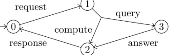
Modal specifications were first introduced in [LT88]. They offer a formalism based on automata to specify some systems by expressing some mandatory and optional transitions. These specifica-tions can then be refined by deciding if some optional parts should be removed or made mandatory. This allows to incrementally design a system by refining it step by step until no variability remains. Consider for example the modal specification depicted in Figure 2.1. It is an automaton with four states labeled 0, 1, 2, and 3, an initial state 0, and some transitions between these states. Observe that contrary to classical automata, there are two kinds of transitions: straight lines are mandatory transitions and dashed lines are the optional ones. This specification describes the behavior of a server which receives some requests and sends a response which may be directly computed or fetched through a query to another server.

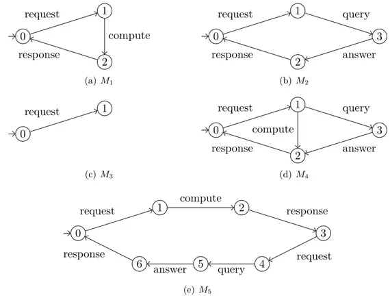
We can also see a modal specification as a characterization of a family—finite or not—of systems, called its models or implementations, represented by automata corresponding to all the possible combinations of implementation choices made by refinement. Some models of the

0 1 2 3 request compute query answer response

(12)

0 1 2 request compute response (a) M1 0 1 2 3 request query answer response (b) M2 0 1 request (c) M3 0 1 2 3 request compute query answer response (d) M4 0 1 2 3 4 5 6

request compute response

request query

answer response

(e) M5

Figure 2.2: Some models of the modal specification of Figure 2.1

example specification presented previously are depicted in Figure 2.2. From the initial state 0 of the specification, there is one mandatory transition, labeled request, so all the models have it. Afterwards, in state 1, there are two optional transitions, which may be realized or not. In M1,

we chose to realize the transition compute but not the query, while we did the opposite in M2.

In M3, we decided to realize none and thus do nothing from state 1. Last, in M4, we implemented

both transitions. Then, the transitions response from state 2 and answer from state 3 are both mandatory, so they are realized in all the models where these states are reached. Finally, M5 shows

that the models of a modal specification have to observe the requirements expressed by the two types of transitions, but not the structure of the specification itself: they can unfold it in order to duplicate some states and make different implementation choices. Therefore, M5 alternates

between computing the result and sending a query to get it. Observe that due to the possibility of unfolding the underlying automaton, the specification has an infinite number of models. For instance, we could build an infinite set consisting of the models realizing the transition compute n times (for any natural number n), then the transition query once (M5 is an example of a such

model for n = 1).

Modal specifications may be based on deterministic or nondeterministic automata. Since the contributions of this thesis are related to deterministic structures, we will now formally define deterministic automata and deterministic modal specifications, as well as the satisfaction relation between a specification and one of its models. We will discuss the choice of using deterministic specifications in Section 2.3.

Definition 1 (Automaton). A deterministic automaton over an alphabet Σ is a tuple (R, r0, λ) where R is the set of states, r0 _{∈ R is the initial state, and λ : R × Σ → R is the partial labeled}

(13)

2.1. Overview and Variants 13

actions a such that λ(r, a) is defined.

Definition 2 (Modal Specification). A deterministic modal specification over an alphabet Σ is a tuple (Q, q0_{, δ,}_{may, must) where Q is the set of states, q}0 _{∈ Q is the initial state, δ : Q × Σ → Q is}

the partial labeled transition map, and may, must : Q → 2Σ _{are the sets of optional and mandatory}

transitions.

We also define a special empty modal specification S⊥, which has no models.

Definition 3 (Satisfaction). An automaton M is a model of a modal specification S, denoted M |= S, if and only if there exists a simulation relation π ⊆ R × Q such that (r0, q0) ∈ π and for any (r, q) ∈ π:

• must(q) ⊆ ready(r) ⊆ may(q);

• for any a ∈ ready(r), we have (λ(r, a), δ(q, a)) ∈ π.

The set of models of S is denoted JS K.

For example, let us look back at the specification in Figure 2.1. The initial state q0 _{is 0 and for}

any state q, the transitions in may(q) \must(q) are depicted with dashed lines while the transitions in may(q) ∩ must(q) are straight lines. Consider the model M5of this specification in Figure 2.2(e):

we can see that the simulation relation is {(0, 0), (1, 1), (2, 2), (3, 0), (4, 1), (5, 3), (6, 2)}.

According to the definition of modal specifications, we could have some specifications with more transitions in must than in may. For example, consider the following specification : ({0}, 0, {(0, a) 7→ 0, (0, b) 7→ 0}, {0 7→ {a}}, {0 7→ {a, b}}). It consists of a single state 0 with two transitions to itself labeled a and b. The transition a is in both may(0) and must(0) while b only belongs to must(0). If we want to build a model of this specification, the must set tells us that we have to realize the two transitions by a and b, but the may set only allows a. Thus, it is impossible to build a model of this specification.

Definition 4(Inconsistency). Given a modal specification S, a state q of S is said to be inconsistent if must(q) 6⊆ may(q) or ready(q) 6= may(q).

A modal specification is said inconsistent if it has an inconsistent state. The specification S_⊥ is consistent.

Theorem 1 (Pruning). Given an inconsistent modal specification S, there exists a consistent modal specification, called normal form of S and denoted ρ(S), with the same models as S.

We can construct ρ(S) by recursion: remove the inconsistent states and all the transitions leading to them, and repeat the process if it has generated some new inconsistencies. Since inconsistent states have incompatible constraints and can not be realized by the models of the specification, removing them does not change its set of models. A more detailed construction along with a proof of correctness are given in [Rac08].

Remark. If the initial state of S is inconsistent (or if an inconsistent state is reachable from the

initial state by taking only must transitions), then ρ(S) = S_⊥.

In consequence, we can now assume, without loss of generality, that all the modal specifications are consistent; whenever a specification may not be consistent, we can simply apply ρ in order to get an equivalent consistent specification. The advantage of having a separate pruning operation ρ instead of requiring directly in the definition of modal specifications that may(q) ⊆ must(q) is that some operations may temporarily generate an inconsistent specification and then use ρ to remove the inconsistencies, rather than building a consistent specification in a single step.

(14)

0 1 2 request compute response (a) 0 1 2 3 request compute query answer response (b)

Figure 2.3: Some refinements of the modal specification of Figure 2.1

Definition 5 (Modal refinement). Given two modal specifications S1 and S2, S1 is a refinement

of S2, denoted S1 ≤ S2, if and only if there exists a simulation relation π ⊆ Q1× Q2 such that

(q0

1, q20) ∈ π and for any (q1, q2) ∈ π:

• may(q1) ⊆ may(q2);

• must(q2) ⊆ must(q1);

• for any a ∈ may(q1), we have (δ(q1, a), δ(q2, a)) ∈ π.

Moreover, for any specification S, S_⊥≤ S.

This definition of refinement is equivalent to thorough refinement, i.e. sets of models inclusion (see [Rac08] for the proof). Note that while most definitions and theorems of this section can be adapted to nondeterministic modal specifications, it is not the case for this one. We give the counter-example in Section 2.3.

Theorem 2. Given two modal specifications S1 and S2, S1 ≤ S2 if and only if JS1K ⊆ JS2K. We depicted in Figure 2.3 two possible refinements of the modal specification of Figure 2.1. In the left one, we removed a transition, query, from the set may. In the right one, we extended the set must by adding the transition query to it.

Variants. Since the introduction of modal specifications in 1988, many variants have been

developed, that we will review now.

Mixed specifications [DGG97] are similar to modal specifications without the consistency assumption. Thus, the case of transitions belonging to the must set but not to the may set is handled explicitly, while in modal specifications it is assumed that a pruning step has been applied beforehand if needed.

Intuitively, the must transitions of modal specifications express a conjunction: all the transitions in the must set have to be realized by the implementations. Several variants of modal specifications have been devised in order to express other kinds of constraints.

Disjunctive modal specifications [LX90] allow expressing a disjunction of must transitions: at least one of the transitions has to be realized. For example, we show in Figure 2.4 a disjunctive variant of the modal specification of Figure 2.1 with a disjunctive-must (d-must) for the transitions

compute and query from state 1. This disjunctive modal specification will have essentially the

same models as the modal specification, except that at least one of the transitions compute and

query has to be realized, thus forbidding models like M3 (Figure 2.2(c)). We will now give a formal

definition of disjunctive modal specifications and their satisfaction relation. Note that we give the definition of the deterministic version of disjunctive modal specifications.

(15)

2.1. Overview and Variants 15 0 1 2 3 request compute query answer response

Figure 2.4: A disjunctive modal specification

Definition 6 (Disjunctive Modal Specification). A deterministic disjunctive modal specification over an alphabet Σ is a tuple (Q, q0_{, δ,}_{may, d-must) where Q is the set of states, q}0 _{∈ Q is the}

initial state, δ : Q × Σ → Q is the partial labeled transition map, may : Q → 2Σ _{is the set of}

optional transitions, and d-must : Q → 22Σ

is a set of disjunctions of mandatory transitions. Definition 7 (Satisfaction). An automaton M is a model of a disjunctive modal specification S, denoted M |= S, if and only if there exists a simulation relation π ⊆ R × Q such that (r0_{, q}0_{) ∈ π}

and for any (r, q) ∈ π:

• ready(r) ⊆ may(q);

• for any must ∈ d-must(q), ready(r) ∩ must 6= ∅; • for any a ∈ ready(r), we have (λ(r, a), δ(q, a)) ∈ π.

One-selecting modal specifications [FS08] offer an exclusive disjunction instead of the inclusive disjunction of disjunctive modal specifications. Thus, if we consider the specification of Figure 2.4 to be a one-selecting modal specification, it would also forbid models like M4 (Figure 2.2(d)) which

realizes both transitions compute and query simultaneously (on the other hand, the model M5

is fine since these two transitions are realized in different states). Moreover, one-selecting modal specifications also offer exclusive disjunctions of may transitions.

Acceptance specifications [Rac08] are an even more expressive extension of modal specifications since they allow expressing arbitrary constraints on the transitions, not just conjunctions or disjunctions. This formalism is the basis of the contributions of this thesis, so we will present it in details in Chapter 3.

Another approach is to use a boolean formula to express the constraints on the transitions instead of sets of may/must/d-must/. . . transitions. Modal specifications with obligations [BK10] accept arbitrary positive boolean formulas and boolean modal specifications [BKL+_{11] extend them}

with negation. If the formulas are in conjunctive normal form without negation, the specification is a disjunctive modal specification, and if the formulas are only conjunctions of actions, the specification is a modal specification. Parametric modal specifications [BKL+_{11] add boolean}

parameters to these specifications.

Definition 8 (Positive Boolean Formula). A positive boolean formula over an alphabet Σ is given by the following grammar:

ϕ::= a | ϕ ∧ ϕ | ϕ ∨ ϕ | > | ⊥ with a ∈ Σ. We denote the set of all positive boolean formulas as B+_.

Given a formula ϕ, the set of actions satisfying the formula, denotedJϕK, is defined as: JaK = {X | a ∈ X } Jϕ ∧ ψK = JϕK ∩ JψK Jϕ ∨ ψK = JϕK ∪ JψK J>K = 2

Σ

(16)

Definition 9 (Modal Specification with Obligations). A deterministic modal specification with obligations over an alphabet Σ is a tuple (Q, q0_{, δ,}_{Ω) where Q is the set of states, q}0 _{∈ Q is the}

initial state, δ : Q × Σ → Q is the partial labeled transition map, and Ω : Q → B+ _{is the set of}

obligations.

Definition 10 (Satisfaction). An automaton M is a model of a modal specification with obliga-tions S, denoted M |= S, if and only if there exists a simulation relation π ⊆ R × Q such that

(r0_{, q}0_{) ∈ π and for any (r, q) ∈ π:}

• ready(r) ∈JΩ(q)K or ready(r) = JΩ(q)K = ∅; • for any a ∈ ready(r), we have (λ(r, a), δ(q, a)) ∈ π.

We now give the definition of boolean modal specifications which is very close to the definition of modal specifications with obligations, but with more expressive formulas:

Definition 11 (Boolean Formula). A boolean formula over an alphabet Σ is given by the following grammar:

ϕ::= a | ¬ϕ | ϕ ∧ ϕ | ϕ ∨ ϕ | > with a ∈ Σ. We denote the set of all boolean formulas as B.

Given a formula ϕ, the set of actions satisfying the formula, denotedJϕK, is defined as: JaK = {X | a ∈ X } J¬ϕK = 2

Σ_\

JϕK Jϕ ∧ ψK = JϕK ∩ JψK Jϕ ∨ ψK = JϕK ∪ JψK J>K = 2

Σ

Definition 12 (Boolean Modal Specification). A deterministic boolean modal specification over an alphabet Σ is a tuple (Q, q0_{, δ,}_{Ω) where Q is the set of states, q}0 _{∈ Q is the initial state,}

δ : Q × Σ → Q is the partial labeled transition map, and Ω : Q → B is the set of obligations. Definition 13 (Satisfaction). An automaton M is a model of a boolean modal specification S, denoted M |= S, if and only if there exists a simulation relation π ⊆ R × Q such that (r0_{, q}0_{) ∈ π}

and for any (r, q) ∈ π:

• ready(r) ∈JΩ(q)K or ready(r) = JΩ(q)K = ∅; • for any a ∈ ready(r), we have (λ(r, a), δ(q, a)) ∈ π.

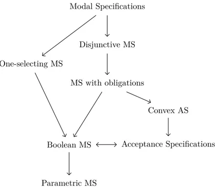
We illustrate the relations between these different specification formalisms in Figure 2.5. Note that this is for deterministic specification formalisms. For nondeterministic specifications, [BDF+_{13] shows that disjunctive modal specifications are equivalent to acceptance specifications,}

hence most formalisms of Figure 2.5 are equivalent in the nondeterministic case, save the parametric extension. The relations between the specification formalisms indicated in Figure 2.5 and convex and acceptance specifications will be justified in Chapter 3.

Logic equivalences. There are some equivalences between specification formalisms and logics

that is, there are constructions to convert an automata-based specification into a logic formula having the same models and vice versa. Modal specifications have been linked to Hennessy-Milner logic (HML) [HM80]: any modal specification has an equivalent HML formula [Lar89] and any consistent and prime HML formula is equivalent to a modal specification [BL92]. Moreover, nondeterministic disjunctive modal specifications are equivalent to HML formulas with greatest fixed points [BDF+_13].

(17)

2.1. Overview and Variants 17 Modal Specifications Disjunctive MS MS with obligations One-selecting MS Boolean MS Parametric MS Convex AS Acceptance Specifications

Figure 2.5: Relations between deterministic specification formalisms

Applications. As hinted in the introduction of this thesis, modal specifications have been

intensively used as a specification formalism for modular system design via the definition of specification theories. They have also been used in different contexts that we briefly mention now.

In [BG00], Kripke structures with modalities are introduced to represent incomplete state spaces. A 3-valued answer is then provided to the model-checking question; the answer unknown corresponds to the situation where the witness paths have a may modality. Other uses of modalities in model-checking have been presented in [CDEG03, HJS01].

Modalities have also been used for software product line modeling [AtBFG10]. The optional behavior encoded by the may modality corresponds to possible features of a product from the family specified by the modal specification.

Modalities have been applied to contract-based design [GR09, BDH+_{12, NITS14]. In essence,}

a contract is a component specification that can be viewed as a pair (A, G) of two specification requirements, where A is an assumption on the environment where the component executes and G is a guarantee on the behavior of the component (given that the assumption is correctly met). This paradigm offers great improvements in system design [BCN+_{12]: it eases component integration}

while enabling compositional design and verification and providing a legal binding between the different suppliers of a development chain.

Extensions. Modal specifications have been extended with input/output actions and

inter-face compatibility notions, based on the approach of interinter-face automata [dAH01]. It was done for both deterministic specifications [LNW07a, RBB+_{09, RBB}+_{11] and nondeterministic ones}

[LV12, BFLV15, CCJK12]. Modal specifications with data [BHB10, BHW11, BLL+_{14] enrich the}

interfaces with data variables.

Many timed extensions have been proposed for modal specifications, such as timed modal specifications [ČGL93], modal event-clock specifications [BLPR09, BLPR12], timed I/O modal specifications [DLL+_{10b], and time-parametric modal specifications [KSL13].}

(18)

Weighted modal specifications [BFJ+_{13] and label-structured modal specifications [BJL}+_12]

extend modal specifications with quantitative properties. A probabilistic extension has been defined in [JL91].

Petri nets decorated with modalities on transitions have been considered in [EHH12, HHM13]. Marked modal specifications [CR12] add reachability properties by means of marked states. We will talk about this formalism and our extension, marked acceptance specifications, in Chapter 4.

2.2 A Modal Specification Theory

We have presented in the previous section the formalism of modal specifications and its semantics via the definitions of the refinement and satisfaction relations. Now, we define some operations on modal specifications to build a modal specification theory as it is done in [RBB+_{11]. As already}

briefly advocated in the introduction of this thesis, this algebra enables modular system design and allows addressing a number of challenges. In what follows, we will motivate precisely each of these operations.

Note also that defining specification theories is the stepping stone for the construction of contract-based theories as advocated in [BDH+_{12]. In this paper, it is shown that given a}

specification theory with refinement, product, conjunction and quotient for a given formalism S, it is possible to derive for free a contract theory for pairs (A, G) of specifications from S with refinement and product.

2.2.1 Conjunction

When specifying a system, it may be easier for a team of system designers to describe the different aspects of a system (function, safety, timing, resource use, etc.) in distinct specifications. This discipline is often referred to as viewpoint design (see [RT14] for a survey). Natural questions arising then are: are these viewpoints consistent that is, do they contradict one another? How can one be sure that all aspects are eventually implemented? These questions call for the support of a conjunction operation on specifications characterizing the common implementations of a set of viewpoints described in some specifications. In particular, inconsistency of viewpoints can be tested by checking if a conjunction has an empty set of models.

Conjunction of modal specifications, also called merge, has been initially studied in [UC04] when silent actions are involved. It has also been considered for labeled transition systems [LV06], for Moore interfaces [HN12], and for interface automata [DHJP08]. In this last paper, it is also argued that supporting conjunction allows merging specifications considered to be similar enough to share a common implementation, hence alleviating the implementation task.

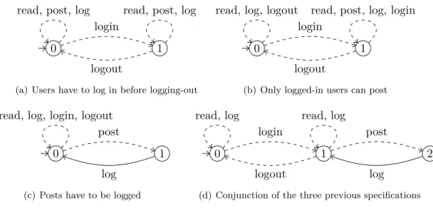
Consider now for example the specifications in Figure 2.6. The goal is to specify the behavior of a simple forum-like server where users may log in, log out, and read and post messages. Moreover, the server may log some information. We want to express three requirements and write a modal specification for each one:

1. Figure 2.6(a): users are initially anonymous; they may log in and log out afterwards; 2. Figure 2.6(b): only logged-in users are allowed to post a message;

3. Figure 2.6(c): the server has to note in the log file when someone posts a message.

Then, we can use the conjunction operation to merge altogether these three viewpoints of the system in order to obtain a single specification, depicted in Figure 2.6(d). If an automaton is

(19)

2.2. A Modal Specification Theory 19

0 1

login logout

read, post, log read, post, log

(a) Users have to log in before logging-out

0 1

login logout

read, log, logout read, post, log, login

(b) Only logged-in users can post

0 1

post log read, log, login, logout

(c) Posts have to be logged

0 1 2

login logout

post log read, log read, log

(d) Conjunction of the three previous specifications

Figure 2.6: Several requirements of a system and their conjunction

an implementation of this specification, we will have the guarantee that it also implements each requirement, and vice versa. Moreover, refinement is preserved by conjunction, so if we refine the specifications, their conjunction will refine the first conjunction.

Definition 14 (Conjunction). Given two modal specifications S1 and S2, their conjunction

S1 ∧ S2 is the normal form of S1& S2 = (Q1 × Q2,(q₁0, q₂0), δ, may, must) where δ((q1, q2), a)

is defined as (δ(q1, a), δ(q2, a)) when both are defined, may((q1, q2)) = may(q1) ∩ may(q2), and

must((q1, q2)) = must(q1) ∪ must(q2).

The conjunction of two modal specifications characterizes precisely the intersection of their sets of models:

Theorem 3. Given two modal specifications S1 and S2, JS1∧ S2K = JS1K ∩ JS2K.

As a consequence, the conjunction operation is commutative and associative. Moreover, since the modal refinement is a thorough refinement, the conjunction is monotonic w.r.t. refinement:

Corollary 1. Given four modal specifications S1, S01, S2, and S02 such that S01 ≤ S1 and S02≤ S2,

S01_{∧ S}02_{≤ S}1∧ S2.

2.2.2 Product

We also want to be able to compose modal specifications by computing their product, which results in a specification where their common transitions have been synchronized. This enables a bottom-up approach to system design: we can start from basic components and compose them together in order to obtain a more complex system.

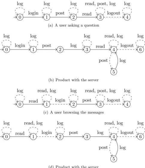
We described in the previous section (Figure 2.6) a server for a message board. We could specify the behavior of some users of this service. For instance, in Figure 2.7(a), we describe a user who wants to ask something: she logs in, posts a message, and then reads the responses, possibly posting other messages. In Figure 2.7(c), we specify another type of user who first browses the board and reads some message, and then may decide to log in and participate in a discussion. We can then compose the specification of a user with the specification of the server (Figure 2.6(d)), as depicted in Figures 2.7(b) and 2.7(d).

(20)

0 login 1 post 2 read 3 logout 4 log log log read, post, log log

(a) A user asking a question

0 1 2 3 4

5

6

login post log _read

post log logout

log log log read, log log

(b) Product with the server

0 read 1 login 2 post 3 logout 4 log read, log log read, post, log log

(c) A user browsing the messages

0 1 2 3 4

5

6

read login post log logout

post log

log read, log log read, log log

(d) Product with the server

(21)

2.2. A Modal Specification Theory 21

Definition 15(Product). Given two modal specifications S1and S2, their product is the modal

spec-ification S1⊗S2= (Q1×Q2,(q₁0, q0₂), δ, may, must) where δ((q1, q2), a) is defined as (δ(q1, a), δ(q2, a)) when both are defined, may((q1, q2)) = may(q1)∩may(q2), and must((q1, q2)) = must(q1)∩must(q2).

The product of modal specifications generalizes the product of models by characterizing the set of the products of models of S1 and S2:

Theorem 4. Given two modal specifications S₁ and S₂, and two automata M₁ _{|= S}₁ and M₂ _{|= S}₂, M1× M2 |= S1⊗ S2.

Moreover, the product is the most precise characterization of the products of models of S1

and S2:

Theorem 5. Given three modal specifications S₁, S₂ and S, if for any M₁ _{|= S}₁ and M₂ _{|= S}₂, M1× M2 |= S, then S1⊗ S2 ≤ S.

The product operation is commutative and associative. It is also monotonic w.r.t. refinement:

Theorem 6. Given four modal specifications S1, S01, S2, and S02 such that S01 ≤ S1 and S02≤ S2,

S01⊗ S02 ≤ S1⊗ S2.

As a result, given an initial design S1⊗S2, the two specifications S1and S2can be independently

refined, potentially by different design teams or suppliers, and then composed in a bottom-up fashion to obtain a correct-by-construction realization of the initial design.

2.2.3 Quotient

The product presented earlier enables a bottom-up approach: one may specify various systems and then compose them together. On the other hand, one may prefer a top-down approach: given the specification of a desired system G and the specification of some pre-existing trustworthy component C (from a library for instance), what is the specification of the system S that we should realize so that its product with C refines G? This is given by the quotient G/C that we consider now in the modal case by following the approach initially developed in [Rac08].

Definition 16 (Quotient). Given two modal specifications S1 and S2, their quotient S1/S2 is the

normal form of S1//S2 = ((Q1× Q2) ∪ {q>}, (q01, q20), δ, may, must) with:

δ((q₁, q₂), a) = (

(δ(q1, a), δ(q2, a)) when both are defined

q_> otherwise               

a_{∈ may((q}1, q2)) ∩ must((q1, q2)) if a ∈ must(q1) ∩ must(q2)

a_{∈ must((q}1, q2)) \ may((q1, q2)) if a ∈ must(q1) \ must(q2)

a∈ may((q1, q2)) \ must((q1, q2)) if a ∈ may(q1) \ must(q1)

a_{∈ may((q}1, q2)) \ must((q1, q2)) if a 6∈ may(q1) ∪ may(q2)

a_{6∈ may((q}1, q2)) ∪ must((q1, q2)) if a ∈ may(q2) \ may(q1)

This quotient operation is dual of the product:

Theorem 7. Given three modal specifications S, S1 and S2, S ≤ S1/S2 if and only if S ⊗S2 ≤ S1.

(22)

Theorem 8. Given two modal specifications S1 and S2, and an automaton M, M |= S1/S2 if

and only if for all M2 |= S2, M × M2|= S1.

Observe that we quantify universally on the models of S2. It is because this reused system

must be seen as a black-box: its implementation is unknown, its reuse is enabled only from the description provided by its specification.

The quotient operation is also crucial for contract satisfaction [BCN+_{12]. As briefly explained}

in the paragraph Applications at the end of Section 2.1, a contract is a pair of specifications (A, G) where A describes some assumptions on the environment of a system M; this system M has to guarantee the satisfaction of G when put in a correct environment satisfying A. More formally, if

E _{|= A then we must have M × E |= G which exactly corresponds to check whether M |= G/A.}

Different problems very similar to synthesizing a quotient exist in the literature. We can first mention the problem of controller synthesis [RW89] considered in the discrete-event systems community. The goal there is to synthesize a subsystem called a controller which aims at enforcing a given specification on a given system. In this context, the system to be controlled is in most cases a deterministic finite automaton [RW89, CL08] whose transitions can be labeled by actions declared uncontrollable, that is the controller cannot forbid them, or unobservable, that is the controller cannot see their occurrence. Quotient as considered in this section is quite different from monolithic controller synthesis. Indeed, we compute quotient of two specifications while monolithic controller synthesis can be interpreted as the quotient of a specification, the control objective, by the system to be controlled. It is more relevant to link quotient with distributed controller synthesis. This was advocated in [AVW03] in which quotient of Mu-calculus formulas

S1/S2 is investigated in order to test the existence of a subcontroller enforcing locally S2 and

globally S1. Their remarkable theoretical contribution is however unusable in practice because of

its complexity cost.

Quotient is also close to computing a protocol converter or an adaptor [YS97, CPS08, MPS12] in order to correct some mismatches between a set of interacting subsystems and thus enforcing a compatibility criterion (deadlock freeness, for instance). The problem has been intensively studied in the service community (see [BBG+_{04, CMP06] for surveys). There again, a clear difference is}

that the description of the system to be adapted is a fixed labeled transition system while our quotient handles specifications, e.g. families, possibly infinite, of systems.

More abstractly, all these previous problems are seen in [VYB+_{11, VPY}+_{15] as solving equations}

of the form:

CkX ∼ G

where the goal is to synthesize the unknown subsystem X that when composed via the operation k with the given context C produces a system which is conform for ∼ to the given objective represented by G. Language equation solving is considered for regular and infinite languages. Actions from the alphabet can either be inputs if they stem from the system environment or outputs when they originate from the system. Composition may correspond to synchronous product with internalization of synchronized actions (see [VYB+_{11] for a survey).}

Links between all these problems have been clearly highlighted in [VYB+_{11, GMW12].}

2.3 Nondeterminism

There are both deterministic and nondeterministic versions of modal specifications. The advantage of nondeterministic specifications is rather clear: they are a strict superset of deterministic

(23)

2.3. Nondeterminism 23 specifications, and thus more expressive. However, nondeterminism has some drawbacks.

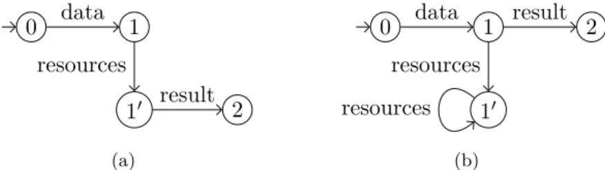
The first problem was mentioned when we defined the refinement relation on modal specifi-cations and proved that it is equivalent to thorough refinement (Theorem 2). This result does not hold for nondeterministic specifications, as shown in [LNW07b]. Indeed, consider the two nondeterministic specifications depicted in Figure 2.8. There are three implementation choices allowed by the specification S: realizing no transition from the initial state, a single transition by a, or two consecutive transitions by a. In each case, the corresponding choice may be made by implementations of T . However, S does not refine T : starting from the pair of initial states (0, 0), there is a may transition by a which may go to the pair (1, 1) or to the pair (1, 2). There is a may transition by a from state 1 of S, but in the first case, it is forbidden by state 1 of T and in the second case, it is in the must set of state 2 of T . Thus, S does not refine T , while its set of models is included in the set of models of T . According to [LNW07b], thorough refinement is decidable, so it is possible to check it directly rather than using modal refinement, but it is co-NP hard, making it unusable for large specifications.

0 1 2 a a (a) S 0 1 2 3 a a a (b) T Figure 2.8: JS K ⊆ JT K but S 6≤ T

The second problem with nondeterministic specifications is that operations are more difficult to define and have a higher complexity—we already saw it for thorough refinement. Consider for instance the quotient operation. We gave a definition of the quotient of deterministic modal specifications in Definition 16, based on the one in [Rac08]. The state space of this quotient is (Q1× Q2) ∪ {q>}. As far as we know, the first definition of the quotient for nondeterministic

modal specifications was given in [BDF+_{13]. The state space of this quotient is 2}Q1×Q2, i.e.,

there is an exponential blow-up for the number of states. The authors add: “we conjecture that the exponential blow-up of the construction is in general unavoidable.” Moreover, the quotient of nondeterministic modal specifications is not homogeneous: the result is a nondeterministic

disjunctive modal specification.

In consequence, although nondeterministic specifications are more expressive, deterministic specifications offer some interesting properties, like a homogeneous quotient and the equivalence between thorough refinement and modal refinement, and the operations on these specifications are simpler to define and much more efficient on large systems.

(24)

(25)

Chapter 3 Acceptance Specifications and

Convex Optimization

We now give a more detailed definition of acceptance specifications and show that this formalism is more expressive than other variants of modal specifications such as disjunctive modal specifications or modal specifications with obligations. Then, we define the operations of conjunction, product, and quotient on acceptance specifications. In Section 3.3, we introduce the first main contribution of this thesis: the definition of a subclass of acceptance specifications, convex-closed acceptance specifications, which allows defining more efficient operations, in particular for the quotient, while being still more expressive than disjunctive modal specifications or modal specifications with obligations. Finally, we give an overview of the Coq mechanization of the theorems given in this last section.

3.1 Semantics

Acceptance trees have been introduced in [Hen85] as a way to represent nondeterministic trees with an underlying deterministic structure. A variant of acceptance trees adapted to automata has been considered in [Rac08] as a specification formalism, called acceptance specifications, which generalizes modal specifications. Instead of expressing two kinds of constraints on transitions—that they are allowed or required—acceptance specifications can express arbitrary constraints on which sets of transitions may be realized by the implementations. Note that the results presented in this section and the next one (Section 3.2) are essentially based on [Rac08].

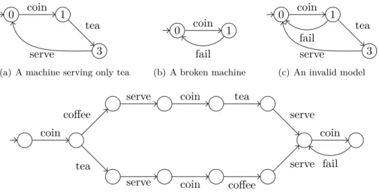
Consider the example of acceptance specification depicted in Figure 3.1. It specifies the behavior of a coffee machine which waits for someone to put a coin and then offers coffee, tea, or both, or indicates a failure. Observe that there is no more two kinds of transitions, but that a set

0 1 2 3 coin coffee tea fail serve serve Acc(0) = {{coin}}

Acc(1) = {{coffee}, {tea}, {coffee, tea}, {fail}} Acc(2) = {{serve}}

Acc(3) = {{serve}}

(26)

0 1

3 coin

tea serve

(a) A machine serving only tea

0 coin 1 fail (b) A broken machine 0 1 3 coin tea fail serve (c) An invalid model coin coffee tea serve serve coin tea serve coin coffee serve coin fail

(d) Machine serving one cup of tea and one cup of coffee

Figure 3.2: Some models of the acceptance specification of Figure 3.1

is associated to each state. For states 0, 2 and 3, there is a unique singleton in the acceptance set, which is equivalent to a single must transition. For state 1 on the other hand, the acceptance set has four elements which means that when implementing the specification, one has to choose one of these elements and realize all the transitions it contains.

For example, when implementing the model in Figure 3.2(a), we selected the set of transitions {tea}, while we chose the set {fail} when implementing the model in Figure 3.2(b). On the other hand, the automaton in Figure 3.2(c) is not a model of the specification: from state 1, it has two transitions, {tea, fail}, and this set does not belong to the acceptance set of the corresponding state in the specification.

It is still possible to unfold a specification when implementing it in order to make different implementation choices in different states which correspond to the same state in the specification. For instance, the automaton of Figure 3.2(d) is a model of the specification which serves exactly one cup of tea and one cup of coffee, in an arbitrary order: if coffee is ordered first, it will then offer only tea and fail afterwards, while if tea is asked first, it will offer coffee before failing. The state 1 of the specification is implemented four times in the model, each implementation realizing a different element of the acceptance set.

The formal definition of acceptance specifications is similar to the definition of modal specifica-tions with the may/must sets replaced by an acceptance set:

Definition 17 (Acceptance Specification). An acceptance specification over an alphabet Σ is a tuple S = (Q, q0_{, δ,}_{Acc) where Q is a finite set of states, q}0 _{∈ Q is the unique initial state,}

δ : Q × Σ → Q is the partial labeled transition map, and Acc : Q → 22Σ associates to each state a set of ready sets called its acceptance set.

We also define a special empty acceptance specification S⊥, which has no models.

The satisfaction relation between an automaton and an acceptance specification is defined as follows:

Definition 18 (Satisfaction). An automaton M satisfies an acceptance specification S, denoted M |= S, if and only if there exists a simulation relation π ⊆ R × Q such that (r0, q0) ∈ π and, for all (r, q) ∈ π:

(27)

3.1. Semantics 27

• ready(r) ∈ Acc(q) and

• for any a ∈ ready(r), we have (λ(r, a), δ(q, a)) ∈ π.

Observe that this definition is similar to Definition 3 of satisfaction for modal specifications with the may/must inclusions replaced by acceptance set membership.

Acceptance specifications are very expressive and are in particular more expressive than modal specifications and many variants such as disjunctive modal specifications and modal specifications with obligations. We give the constructions transforming these specifications into acceptance specifications:

Theorem 9. Given a modal specification S, there exists an acceptance specification S_Acc such thatJS K = JSAccK.

Proof. If S = (Q, q0_{, δ,}_{may, must), let S}_Acc _{= (Q, q}0_{, δ,}_{Acc) where:}

Acc(q) = {X | must(q) ⊆ X ⊆ may(q)} We now prove that these two specifications have the same models.

(⇒) Let M be a model of S. There is a simulation relation π ⊆ R × Q. We prove that M is a model of SAcc using the same simulation relation. We thus know by hypothesis that (r0, q0) ∈ π.

For any (r, q) ∈ π and a ∈ ready(r):

• ready(r) ∈ Acc(q): we know that must(q) ⊆ ready(r) ⊆ may(q); thus ready(r) ∈ Acc(q) by definition of Acc;

• (λ(r, a), δ(q, a)) ∈ π by hypothesis: S and SAcc have the same transition map.

(⇐) Let M be a model of SAcc. There is a simulation relation π ⊆ R × Q. We prove that M

is a model of S using the same simulation relation. We thus know by hypothesis that (r0_{, q}0_{) ∈ π.}

• must(q) ⊆ ready(r) ⊆ may(q): we know that ready(r) ∈ Acc(q); thus must(q) ⊆ ready(r) ⊆ may(q) by definition of Acc;

Theorem 10. Given a disjunctive modal specification S, there exists an acceptance specification SAcc such that JS K = JSAccK.

Proof. If S = (Q, q0_{, δ,}_{may, d-must), let S}_Acc _{= (Q, q}0_{, δ,}_{Acc) where:}

Acc(q) = {X | X ⊆ may(q) ∧ ∀ must ∈ d-must(q), X ∩ must 6= ∅} We now prove that these two specifications have the same models.

• ready(r) ∈ Acc(q): we know that ready(r) ⊆ may(q) and for any must ∈ d-must(q), ready(r) ∩ must 6= ∅; thus ready(r) ∈ Acc(q) by definition of Acc;

(28)

• ready(r) ∈ may(q): we know that ready(r) ∈ Acc(q) and by definition of Acc, ready(r) ∈ may(q);

• ∀ must ∈ d-must(q), ready(r) ∩ must 6= ∅: we know that ready(r) ∈ Acc(q) and conclude by definition of Acc;

Theorem 11. Given a modal specification with obligations S, there exists an acceptance specifica-tion SAcc such that JS K = JSAccK.

Proof. If S = (Q, q0_{, δ,}_{Ω), let S}_Acc _{= (Q, q}0_{, δ,}_{Acc) where:}

Acc(q) =

(

{X | X ∈JΩ(q)K ∧ X ⊆ ready(q)} ifJΩ(q)K 6= ∅

{∅} ifJΩ(q)K = ∅

We now prove that these two specifications have the same models.

• ready(r) ∈ Acc(q): if JΩ(q)K = ∅, ready(r) = ∅ by hypothesis and then ready(r) ∈ Acc(q). Otherwise, ready(r) ∈JΩ(q)K by hypothesis. Thus ready(r) ∈ Acc(q) by definition of Acc; • (λ(r, a), δ(q, a)) ∈ π by hypothesis: S and SAcc have the same transition map.

• ready(r) ∈ JΩ(q)K or ready(r) = JΩ(q)K = ∅: by hypothesis, ready(r) ∈ Acc(q). Either JΩ(q)K = ∅ and then ready(r) ∈ Acc(q) implies ready(r) = ∅, or ready(r) ∈ JΩ(q)K by definition of Acc;

Note that these transformations to acceptance specifications have an exponential blow-up, since they enumerate all the allowed sets of actions (for instance all the sets between must(q) and may(q) for the modal case). We will address this inefficiency in Section 3.3.

There are some acceptance specifications that may not be represented by modal specifications, disjunctive modal specifications or modal specifications with obligations, such as the one of Figure 3.1. Indeed, in state 1 of this specification, there is a disjunction between the actions coffee and tea (i.e., there can be one, the other, or both), and an exclusive disjunction between these actions and the action fail. None of these three formalisms allow to express such constraints. Thus, acceptance specifications are strictly more expressive than these formalisms.

However, boolean modal specifications are expressive enough to be equivalent to acceptance specifications:

(29)

3.1. Semantics 29

Theorem 12. Given a boolean modal specification S, there exists an acceptance specification S_Acc such that JS K = JSAccK.

Proof. The construction of the acceptance specification and the proof are the same as for modal

specifications with obligations (Theorem 11) as the proof does not use any information specific to the logic used (i.e., it works for any logic as long as there is a functionJ.K generating a set of sets of actions and a similar definition of satisfaction).

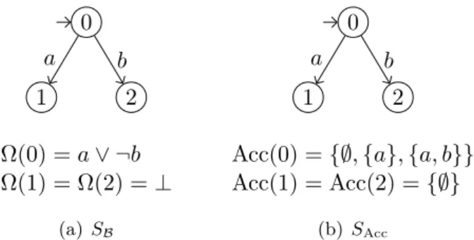
Theorem 13. Given an acceptance specification S, there exists a boolean modal specification S_B such that JS K = JSBK.

Proof. If S = (Q, q0_{, δ,}_{Acc), let S}

B = (Q, q0, δ,Ω) where: Ω(q) = M X∈Acc(q)   ^ a∈X a∧ ^ a6∈X ¬a  

with ⊕ the exclusive disjunction operation (i.e., ϕ ⊕ ψ = (ϕ ∨ ψ) ∧ ¬(ϕ ∧ ψ)). We now prove that these two specifications have the same models.

(⇒) Let M be a model of S. There is a simulation relation π ⊆ R × Q. We prove that M is a model of SB using the same simulation relation. We thus know by hypothesis that (r0, q0) ∈ π.

• ready(r) ∈JΩ(q)K: by hypothesis, ready(r) ∈ Acc(q), thus ready(r) satisfies Ω(q) for the element of the exclusive disjunction where X = ready(q);

• (λ(r, a), δ(q, a)) ∈ π by hypothesis: S and SB have the same transition map.

(⇐) Let M be a model of SB. There is a simulation relation π ⊆ R × Q. We prove that M is

a model of S using the same simulation relation. We thus know by hypothesis that (r0_{, q}0_{) ∈ π.}

• ready(r) ∈ Acc(q): by hypothesis, ready(r) ∈JΩ(q)K, so there is an X ∈ Acc(q) such that the elements of ready(r) are in X (V

a∈Xa) and the elements not in ready(r) are not in X

(V

a6∈Xa), thus X = ready(r) and then ready(r) ∈ Acc(q);

• (λ(r, a), δ(q, a)) ∈ π by hypothesis: S and SB have the same transition map.

We now define the refinement relation between two acceptance specifications. It is similar to the definition of refinement between modal specifications (Definition 5); inclusion of the acceptance sets replaces the inclusions of may and must sets.

Definition 19 (Refinement). Given two acceptance specifications S₁ and S₂, S₁ is a refinement of S2, denoted S1 ≤ S2, if and only if there exists a simulation relation π ⊆ Q1× Q2 such that

(q0

1, q20) ∈ π and for all pairs (q1, q2) ∈ π:

• Acc1(q1) ⊆ Acc2(q2) and

• for any a ∈ ready(q1), we have: (δ1(q1, a), δ2(q2, a)) ∈ π.

Moreover, for any specification S, S⊥≤ S.

The refinement of acceptance specifications is also a thorough refinement: it is equivalent to the inclusion of the sets of models.

(30)

Theorem 14. Given two acceptance specifications S1 and S2, S1≤ S2 if and only if JS1K ⊆ JS2K.

Proof. (⇒) Suppose that S1 ≤ S2 and M |= S1 thanks respectively to the simulation relations

π and π1. Define π2 such that (r, q2) ∈ π2 if and only if there exists a state q1 in S1 such that

(r, q1) ∈ π1 and (q1, q2) ∈ π. We prove that M |= S2 thanks to π2:

• if (r, q1) ∈ π1 then ready(r) ∈ Acc1(q1) by Definition 18; moreover, if (q1, q2) ∈ π then

Acc1(q1) ⊆ Acc2(q2) by Definition 19. As a result, ready(r) ∈ Acc2(q2);

• for any a ∈ ready(r), if (r, q1) ∈ π1 then (λ(r, a), δ1(q1, a)) ∈ π1 by Definition 18;

more-over, if (q1, q2) ∈ π then (δ1(q1, a), δ2(q2, a)) ∈ π by Definition 19. As a result, we have:

(λ(r, a), δ2(q2, a)) ∈ π2.

(⇐) Suppose that JS1K ⊆ JS2K. Define π such that (q10, q02) ∈ π and for all (q1, q2) ∈ π, if

δ1(q1, a) and δ2(q2, a) are defined then (δ1(q1, a), δ2(q2, a)) ∈ π. We prove that S1 ≤ S2 thanks

to π.

Observe first that if δ1(q1, a) is defined then δ2(q2, a) is also defined; this is a direct consequence

to the fact that when δ1(q1, a) is defined, the transition can be included in some models which are

also models of S2 and thus δ2(q2, a) is defined. Then, for any (q1, q2) ∈ π:

• for all X ∈ Acc1(q1), there exists an M |= S1 such that (r, q1) ∈ π1 and ready(r) = X. As

JS1K ⊆ JS2K, M is also a model of S2 and necessarily ready(r) ∈ Acc2(q2). Consequently, Acc1(q1) ⊆ Acc2(q2);

• by definition of π, for any a ∈ ready(q1), we have (δ1(q1, a), δ2(q2, a)).

As a result, according to Definition 19, we have S1≤ S2.

We saw that modal specifications could have inconsistent states, which allowed us to give simpler definitions to some operations and then apply a pruning operation in order to ensure a well-formedness property on modal specifications. Similarly, there may be some inconsistencies in acceptance specifications:

• Acc-consistency. A state q is Acc-consistent when Acc(q) 6= ∅.

• δ, Acc-consistency. A state q is δ, Acc-consistent when, for any action a ∈ Σ, δ(q, a) is defined if and only if there exists an X ∈ Acc(q) such that a ∈ X, i.e., ready(q) =SAcc(q). Remark. It is easy to confuse Acc(q) = ∅ and Acc(q) = {∅}, although these two acceptance sets

have very different meanings. Assume that we have a model M of an acceptance specification S with a simulation relation π, and a state q of S.

If Acc(q) = ∅, q cannot belong to any pair of π since Definition 18 requires ready(r) ∈ Acc(q), which is impossible when Acc(q) = ∅.

On the other hand, if Acc(q) = {∅}, there may be a pair (r, q) ∈ π, which implies ready(r) = ∅, i.e., that there are no outgoing transitions from r.

Definition 20(Normal form). An acceptance specification is in normal form if it is Acc-consistent and δ, Acc-consistent in every state q. Moreover, S⊥ is in normal form.

We demonstrate in Algorithm 1 how to remove the inconsistent states from an acceptance specification and we prove that the resulting specification is in normal form and has the same models as S:

(31)

3.2. An Acceptance Specification Theory 31 Algorithm 1ρ(S: AS): AS 1: if _{∃q, Acc(q) = ∅ then} 2: if q= q0 then 3: return S_⊥ 4: else 5: δ0= {(q0, a) 7→ δ(q0, a) | δ(q0, a) defined ∧ δ(q0, a) 6= q} 6: Acc0 = {q0 7→ {X | X ∈ Acc(q0) ∧ ∀a ∈ X, δ(q0, a) 6= q}} 7: return ρ((Q \ {q}, q0, δ0,Acc0))

8: end if 9: end if

10: if _{∃q, ready(q) 6=}SAcc(q) then

11: δ0 = {(q0, a) 7→ δ(q0, a) | δ(q0, a) defined ∧ a ∈SAcc(q0)}

12: Acc0= {q0 7→ {X | X ∈ Acc(q0) ∧ ∀a ∈ X, δ(q, a) defined}} 13: return ρ((Q, q0, δ0,Acc0))

14: end if

15: return S

Theorem 15. For any acceptance specification S, ρ(S) is in normal form and is equivalent to S. Proof. (normal form) The base case of the recursive definition of ρ is that there is no state q

such that Acc(q) = ∅ or ready(q) 6= SAcc(q). This implies that if ρ terminates, the returned

specification is Acc-consistent and δ, Acc-consistent, hence in normal form. Each time the function ρ is recursively called, its parameter has fewer states, fewer transitions or smaller acceptance sets. Considering that acceptance specifications are finite, ρ is terminating.

(equivalence) By induction:

• In the base case (line 15), the specification S itself is returned.

• For the first recursive call (line 7), we remove from S the state q and the transitions from other states towards q. Since the acceptance set of q is empty, no model of S can implement q, so the specification passed to the recursive call has the same models as S.

• For the second recursive call (line 13), we removed some transitions which were not allowed by the corresponding acceptance set, and thus could not be realized by any model (the condition ready(r) ∈ Acc(q) would not be satisfiable), as well as elements of the acceptance set containing actions for which δ is not defined, which could not be realized in any model either. Thus, the specification passed to the recursive call also has the same models as S. As a result of Theorem 15, from now on and without loss of generality, we assume that acceptance specifications are in normal form.

3.2 An Acceptance Specification Theory

We now show how the operations defined on modal specifications—namely conjunction, product, and quotient—can be extended to acceptance specifications.

3.2.1 Conjunction

The conjunction of acceptance specifications is similar to the conjunction of modal specifications; computing the acceptance sets simply consists in keeping the common elements of the acceptance