Determination of Forces from a Potential in Molecular Dynamics

HAL Id: hal-00924263

https://hal-mines-paristech.archives-ouvertes.fr/hal-00924263

Submitted on 6 Jan 2014

HAL is a multi-disciplinary open access

archive for the deposit and dissemination of

sci-entific research documents, whether they are

pub-lished or not. The documents may come from

teaching and research institutions in France or

L’archive ouverte pluridisciplinaire HAL, est

destinée au dépôt et à la diffusion de documents

scientifiques de niveau recherche, publiés ou non,

émanant des établissements d’enseignement et de

recherche français ou étrangers, des laboratoires

Determination of Forces from a Potential in Molecular

Dynamics

Bernard Monasse, Frédéric Boussinot

To cite this version:

Bernard Monasse, Frédéric Boussinot. Determination of Forces from a Potential in Molecular

Dynam-ics. 2014. �hal-00924263�

Determination of Forces from a Potential

in Molecular Dynamics

(note)

Bernard Monasse

Mines-ParisTech, Cemef

Frédéric Boussinot

Mines-ParisTech, Cemef

January 2014

In Molecular Dynamics (MD), the forces applied to atoms derive from potentials which describe the energy of bonds, valence angles, torsion an-gles, and Lennard-Jones interactions of which molecules are made. These definitions are classic; on the contrary, their implementation in a MD system which respects the local equilibrium of mechanical conditions is usually not described. The precise derivation of the forces from the po-tential and the proof that their application preserves energy is the object of this note. This work is part of the building of a multi-scale MD system, presently under development.

Keywords. Molecular Dynamics ; Force-Fields ; Potentials ; Forces.

1

Introduction

Numerical simulation at atomic scale predicts system states and properties from a limited number of physical principles, using a numerical resolution method implemented with computers. In Molecular Dynamics (MD) [2] systems are organic molecules, metallic atoms, or ions. We concentrate on organic molecules, but our approach could as well apply to other kinds of systems. The goal is to determine the temporal evolution of the geometry and energy of atoms.

At the basis of MD is the classical (newtonian) physics, with the fundamental equation:

− →

F = m−→a (1)

where−→F is the force applied to a particle of mass m and −→a is its acceleration (second derivative of the variation of the position, according to time).

A force-field is composed of several components, called potentials (of bonds, valence angles, dihedral angles, van der Waals contributions, electrostatic contri-butions, etc.) and is defined by the analytical form of each of these components, and by the parameters caracterizing them. The basic components used to model molecules are the following:

• atoms, with 6 degrees of freedom (position and velocity);

• bonds, which link two atoms belonging to the same molecule; a bond between two atoms a, b tends to maintain constant the distance ab. • valence angles, which are the angle formed by two adjacent bonds ba et bc

in a same molecule; a valence angle tends to maintain constant the angle c

abc. A valence angle is thus concerned by the positions of three atoms. • torsion angles (also called dihedral angles) are defined by four atoms a, b, c, d

consecutively linked in the same molecule: a is linked to b, b to c, and c to d; a torsion angle tends to priviledge particular angles between the planes abc and bcd. These particular angles are the equilibrium positions of the torsion potential (minimal energies). In most cases, they are Trans (angle of 180◦_{), Gauche (60}◦_{) or Gauche’ (−60}◦_).

• van der Waals interactions apply between two atoms which either belong to two different molecules, or are not linked by a chain of less than three (or sometimes, four) bonds, if they belong to the same molecule. They are pair potentials.

All these potentials depend on the nature of the concerned atoms and are parametrized differently in specific force-fields. Molecular models can also con-sider electrostatic interactions (Coulomb’s law) which are pair potentials, as van der Waals potentials are; their implementation is close to van der Waals potentials, with a different dependence to distance.

Intra-molecular forces (bonds, valence angles, torsion angles) as well as inter-molecular forces (van der Waals) are conservative: the work between two points does not depend on the path followed by the force between these two points. Thus, forces can be defined as derivatives of scalar fields. From now on, we consider that potentials are scalar fields and we have:

− →

F (r) = −−→∇U (r) (2)

where r denotes the coordinates of the point on which the force−→F (r) applies, and U is the potential from which the force derives.

The work presented here is part of a MD system presently under development[1]; the defined forces and their implementations have been tested with it.

Structure of the text

Bonds are considered in Section 2, valence angles in Section3, torsion angles in Section4, and finally Lennard-Jones potentials in Section5. Section6 sum-marises the force definitions, and Section 7concludes the text. A summary of the notations used in the paper is given in the Annex.

2

Bonds

A bond models a sharing of electrons between two atoms which produces a force between them. This force is the derivative of the bond potential defined between the two atoms. Fig. 2.1shows a (attractive) force produced between two linked atoms a and b.

Figure 2.1: Attractive bond between two linked atoms

A harmonic bond potential is a scalar field U which defines the potential energy of two atoms placed at distance r as:

U (r) = k(r − r0)2 (3)

where k is the strength of the bond and r0 is the equilibrium distance (the

distance at which the force between the two atoms is null). We thus have: ∂U (r)

∂r = 2k(r − r0) (4)

The partial derivative of U according to the position ra of a is:

∂U (r) ∂ra = ∂U (r) ∂r . ∂r ∂ra . (5) But: ∂r ∂ra = 1 (6) We thus have: ∂U (r) ∂ra = 2k(r − r0) (7)

Let a and b be two atoms, and −→u = norm(−→ba) be the normalization of vector −

→

ba. The force produced on atom a is: − → fa= − ∂U (r) ∂ra .−→u = −2k(r − r0).−→u (8)

and the one on b is the opposite, according to the action/reaction principle: − → fb = − − → fa (9)

Therefore, if r > r0, the force on a is a vector whose direction is opposite to −→u

and tends to bring a and b closer (attractive force), while it tends to bring them apart (repulsive force) when r < r0.

According to the definition of −→fa and

− →

fb, the sum of the forces applied to a

and b is null (i.e. equilibrium of forces): − → fa+ − → fb = 0 (10)

Note that no torque is produced as the two forces are colinear.

3

Valence Angles

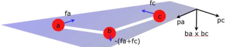
Valence angles tend to maintain at a fixed value the angle between three atoms a, b and c such that a is linked to b and b to c, as shown on Fig. 3.1.

Figure 3.1: Valence angle

The forces applied to the three atoms all belong to the plane abc defined by the points a, b, c.

A harmonic valence potential is a scalar field U which defines the potential energy of an atom configuration forming a valence angle θ by:

U (θ) = k(θ − θ0)2 (11)

where k is the strength of the valence angle and θ0 is the equilibrium angle (the

one for which energy is null). The partial derivative of U according to the angle θ is thus:

∂U (θ)

The partial derivative of U according to the position ra of a is: ∂U (θ) ∂ra = ∂U (θ) ∂θ . ∂θ ∂ra (13) that is: ∂U (θ) ∂ra = 2k(θ − θ0). ∂θ ∂ra (14) As a describes a circle with radius |ab|, centered on b, we have1

: ∂θ

∂ra

= 1

|ab| (15)

Let −→pa be the normalized vector in the plane abc, orthogonal to

− → ba : − →_p a = norm( − → ba × (−→ba ×−→bc)) (16) The force applied on a is then:

− → fa = − ∂U (θ) ∂ra .−→pa = −2k(θ − θ₀)/|ab|.−→pa (17)

In the same way, the force applied on c is: −

→

fc = −2k(θ − θ0)/|bc|.−→pc (18)

where −→pc is the normalized vector in plane abc, orthogonal to

− → cb : − →_p c = norm( − → cb × (−→ba ×−→bc)) (19) The sum of the forces should be null:

− → fa+ − → fb + − → fc = 0 (20)

Thus, the force applied to b is: − → fb = − − → fa− − → fc (21)

3.1

Torques

Let us now consider torques (moment of forces). The torque exerted by−→fa on

b is−→ba ×−→fa and the torque exerted by

− → fc on b is − → bc ×−→fc. As − → ba and −→fa are

orthogonal, one has2

: |−→ba ×−→fa| = |

− →

ba||−→fa| = |ba|| − 2k(θ − θ0)/|ab|| = |2k(θ − θ0)| (22)

1

The length of an arc of circle is equal to the product of the radius by the angle (in radians) corresponding to the arc of circle.

2

For the same reasons:

|−→bc ×−→fc| = |2k(θ − θ0)| (23)

Thus, the two vectors−→ba ×−→fa and

− →

bc ×−→fc have the same length. As they are

by construction in opposite directions, the sum of the two torques on b is null: − → ba ×−→fa+ − → bc ×−→fc = 0 (24)

As a consequence, no rotation around b can result from the application of the two forces−→fa and

− → fc.

4

Torsion Angles

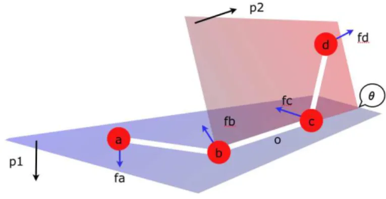
A torsion angle θ defined by four atoms a, b, c, d is shown on Fig. 4.1. In the OPLS [3] force-field, as in many other force-fields, potentials of torsion angles have a “triple-cosine” form. This means that the potential U of a torsion angle θ is defined by3

:

U (θ) = 0.5[A1(1 + cos(θ)) + A2(1 − cos(2θ)) + A3(1 + cos(3θ)) + A4] (25)

Figure 4.1: Torsion angle θ

The partial derivative of the torsion angle potential according to the position ra of a is: ∂U (θ) ∂ra = ∂U (θ) ∂θ . ∂θ ∂ra (26) The partial derivative of the potential according to the angle θ is:

∂U (θ)

∂θ = 0.5(−A1sin(θ) + 2A2sin(2θ) − 3A3sin(3θ)) (27) = −0.5(A1sin(θ) − 2A2sin(2θ) + 3A3sin(3θ)) (28)

3

4.1

Forces on a and d

Let us call θ1 the angle cabc. Atom a turns around direction bc, on a circle of

radius |ab|sin(θ1). The partial derivative of θ according to the position of a is:

∂θ ∂ra = 1 |ab|sin(θ1) (29) We thus have: ∂U (θ) ∂ra = −0.5 |ab|sin(θ1)

(A1sin(θ) − 2A2sin(2θ) + 3A3sin(3θ)) (30)

Similarly, for atom d, noting θ2the angle cbcd :

∂U (θ) ∂rd

= −0.5

|cd|sin(θ2)

(A1sin(θ) − 2A2sin(2θ) + 3A3sin(3θ)) (31)

Let −→p1the normalized vector orthogonal to the plane abc, and −→p2the normalized

vector orthogonal to the plane bcd (the angle between −→p1 and −→p2 is θ):

− → p1= norm( − → ba ×−→bc) (32) − → p2= norm( − → cd ×−→cb) (33)

The force applied on a is: −

→ fa =

0.5 |ab|sin(θ1)

(A1sin(θ) − 2A2sin(2θ) + 3A3sin(3θ)).−→p1 (34)

In the same way, the force applied on d is: −

→ fd=

0.5 |cd|sin(θ2)

(A1sin(θ) − 2A2sin(2θ) + 3A3sin(3θ)).−→p2 (35)

4.2

Forces on b and c

We now have to determine the forces−→fb and

− →

fc to be applied on b and c. The

equilibrium conditions imply two constraints: (A) the sum of the forces has to

be null: _−→ fa+ − → fb+ − → fc+ − → fd= 0 (36)

and (B) the sum of torques also has to be null4

. Calling o the center of bond bc, this means: − → oa ×−→fa+ − → od ×−→fd+ − → ob ×−→fb+ −→oc × − → fc = 0 (37) From (37) it results: (−→ob +−→ba) ×−→fa+ (−→oc + − → cd) ×−→fd+ − → ob ×−→fb+ −→oc × − → fc = 0 (38) 4

It is not possible to simply define−→fb= − −→

faand−→fc= −−→fd, as the sum of torques would be non-null, thus leading to an increase of potential energy.

and: (−−→oc +−→ba) ×−→fa+ (−→oc + − → cd) ×−→fd− −→oc × − → fb+ −→oc × − → fc = 0 (39) which implies: − → oc × (−−→fa+ − → fd− − → fb+ − → fc) + − → ba ×−→fa+ − → cd ×−→fd = 0 (40) From (36) it results: −−→fa+ − → fd− − → fb+ − → fc = 2( − → fd+ − → fc) (41)

Substituting (41) in (40), one gets: − →_{oc × (2(}−→_f d+ − → fc)) + − → ba ×−→fa+ − → cd ×−→fd= 0 (42) thus: 2−→oc ×−→fd+ 2−→oc × − → fc+ − → ba ×−→fa+ − → cd ×−→fd= 0 (43) which implies: 2−→oc ×−→fc = −2−→oc × − → fd− − → cd ×−→fd− − → ba ×−→fa (44)

and we finally get the condition that the torque from−→fc should verify in order

(37) to be true: − →_{oc ×}−→_f c = −(−→oc × − → fd+ 0.5 − → cd ×−→fd+ 0.5 − → ba ×−→fa) (45) Let us state: − → tc = −(−→oc × − → fd+ 0.5 − → cd ×−→fd+ 0.5 − → ba ×−→fa) (46)

Equation −→oc × −→x = −→tc has an infinity of solutions in −→x , all having the same

component perpendicular to −→oc. We thus simply choose as solution the force perpendicular to −→oc defined by:

− →

fc = (1/|oc|2)−→tc × −→oc (47)

Equation (45) is verified because: − →_{oc ×}−→_f c = (1/|oc|2)−→oc × (−→tc × −→oc) (48) thus5 : − →_{oc ×}−→_{fc = (1/|oc|}2_)|oc|2−→_t c =−→tc (49)

The value of−→fb is finally deduced from equation (36) stating the equilibrium

of forces: _−→ fb = − − → fa− − → fc− − → fd (50)

We have thus determined four forces−→fa,

− → fb, − → fc, − →

fdwhose sum is null (36) and

whose sum of torques is also null (37).

5

5

Lennard-Jones Potentials

A Lennard-Jones (LJ) potential U (r) between two atoms placed at distance r is defined by6 : U (r) = 4ǫ[(σ r) 12 − (σ r) 6 ] (51)

In this definition, parameter σ is the distance at which the potential is null, and parameter ǫ is the minimum of the potential (corresponding to the maximum of the attractive energy).

Stating A = σ12_{and B = σ}6_{, Eq. (51) becomes:}

U (r) = 4ǫ( A r12 −

B

r6) (52)

The partial derivative of U according to distance is thus: ∂U (r) ∂r = 4ǫ(−12 A r13 + 6 B r7) (53) = 24ǫ(−2 A r13 + B r7) (54) = 24ǫ r (−2 A r12 + B r6) (55) = −24ǫ r (2( σ r) 12 − (σ r) 6 ) (56)

Let a and b be two atoms. The force on a is: − → fa = 24ǫ r (2( σ r) 12 − (σ r) 6 ).−→u (57)

where −→u is the normalization of −→ba. From the action/reaction principle, one deduces that the force on b should be the opposite of the force on a:

− → fb = − − → fa (58)

According to the definition of −→fa and

− →

fb, the sum of the forces applied to a

and b is null: _−→

fa+

− →

fb = 0 (59)

Note that, as for bonds, no torque is produced because the two forces are col-inear.

6

Resume

The forces defined in the previous sections are summed up in the following table:

6

Bond ab 8 −→fa = −2k(r − r₀).−→u 9 −→fb = −

− → fa

Valence abc 17 −→fa = −2k(θ − θ₀)/|ab|.−→pa 21 −→fb = − − → fa− − → fc 18 −→fc = −2k(θ − θ0)/|bc|.−→pc

Torsion abcd 34 −→fa =_|ab|sin(θ0.5

1)(A1sin(θ) − 2A2sin(2θ) + 3A3sin(3θ)).−

→ p1 50 −→fb = − − → fa− − → fc − − → fd 47 −→fc = (1/|oc|2). − → tc × −→oc 35 −→fd =_|cd|sin(θ0.5

2)(A1sin(θ) − 2A2sin(2θ) + 3A3sin(3θ)).−

→_p 2 LJ ab 57 −→fa =24ǫ_r (2( σ r) 12 − (σ r) 6 ).−→u 58 −→fb = − − → fa

Bond In Eq. 8, k is the bond strength constant, r is the distance between atoms a and b, and r0is the equilibrium distance, for which energy is null. Vector

−

→_{u is defined by −}→_{u = norm(}−→_ba).

Valence In17and18, k is the angle strength constant, θ is the angle cabc, and θ0is

the equilibrium angle, for which energy is null. In17, −→pa is defined by −→pa =

norm(−→ba × (−→ba ×−→bc)). In18, −→pc is defined by −→pc = norm(

− →

cb × (−→ba ×→−bc)). Torsion In 34 and 35, θ is the torsion angle, θ1 is the angle cabc, θ2 is the angle

c

bcd and A1, A2 and A3are the parameters which define the “three-cosine”

form of the torsion angle. Vector −→p1 is defined by −→p1 = norm(

− → ba ×−→bc) and −→p2= norm( − →

cd ×−→cb). In47, o is the middle of bc and−→tc is defined by

− → tc = −(−→oc × − → fd+ 0.5 − → cd ×−→fd+ 0.5 − → ba ×−→fa).

LJ In57, σ is the distance at which the potential is null and ǫ is the depth of the potential (minimum of energy). As for bonds, one has −→u = norm(−→ba). In each case (bond, valence, torsion, LJ interaction), the sum of the forces that are applied to atoms is always null (Eq. (10), (20), (36), (59)). Moreover, no torque is induced by application of these forces: no torque is produced by bonds and LJ interactions, as the produced forces are colinear; we have verified in Sec. 3.1that no torque is produced by valence angles (24); for torsion angles, we have chosen the forces in such a way that the sum of the forces and the global sum of torques are always null (37). This means that no energy is ever added by the application of the forces during the simulation process.

7

Conclusion

We have precisely defined the forces that apply on atoms in MD simulations. The definitions are given in a purely vectorial formalism (no use of a specific

coordinate system). We have shown that the sum of the forces and the sum of the torques are always null, which means that the energy of molecular systems is preserved while the forces are applied.

References

[1] MDRP Site. http://mdrp.cemef.mines-paristech.fr.

[2] M. P. Allen and D. J. Tildesley. Computer Simulation of Liquids. Oxford, 1987.

[3] W. Damm, A. Frontera, J. Tirado-Rives, and W.L. Jorgensen. OPLS All-atom Force Field for Carbohydrates. J. Comput. Chem., 16(18):1955–1970, 1997.

A

Notations

• if a and b are two atoms, we note−→ab the vector with origin a and end b; the distance between the two atoms is noted |ab|.

• The null vector is noted 0.

• The length of vector −→u is noted |−→u |. One thus has: |−→ab| = |ab|. • Multiplication of −→u by the scalar n is noted n.−→u , or more simply n−→u . • The vectorial product of −→u and −→v is noted −→u × −→v .

• The scalar product of −→u and −→v is noted −→u • −→v .

• We write −→u ⊥−→v when −→u and −→v are orthogonal (−→u • −→v = 0).

• We note norm(−→u ) the normalized vector from −→u (same direction, but length equal to 1) defined by norm(−→u ) = (1/|−→u |).−→u .