Comparative study of methods for optimization of electromagnetic devices with uncertainty

Science Arts & Métiers (SAM)

is an open access repository that collects the work of Arts et Métiers Institute of

Technology researchers and makes it freely available over the web where possible.

This is an author-deposited version published in: https://sam.ensam.eu Handle ID: .http://hdl.handle.net/10985/13420

To cite this version :

Siyang DENG, Stéphane BRISSET, Stéphane CLENET - Comparative study of methods for optimization of electromagnetic devices with uncertainty - COMPEL-The international journal for computation and mathematics in electrical and electronic engineering Vol. 37, n°2, p.704717 -2018

Any correspondence concerning this service should be sent to the repository Administrator : [email protected]

COMPARATIVE STUDY OF METHODS FOR OPTIMIZATION OF

ELECTROMAGNETIC DEVICES WITH UNCERTAINTY

Siyang DENG, Stéphane BRISSET and Stéphane CLENET

Univ. Lille, Centrale Lille, Arts et Metiers ParisTech, HEI, EA 2697 - L2EP – Laboratoire

d’Electrotechnique et d’Electronique de Puissance, F-59000 Lille, France

E-mail: [email protected]

Abstract. This paper compares different probabilistic optimization methods dealing with uncertainties. Reliability-Based Design Optimization is presented as well as various approaches to calculate the probability of failure. They are compared in terms of precision and number of evaluations on mathematical and electromagnetic design problems to highlight the most effective methods.

Keywords: Reliability-based design optimization, uncertainty, reliability, safety transformer.

1 INTRODUCTION

In most optimization problems, the variables are usually considered as deterministic, i.e. without any variability. This traditional Deterministic Design Optimization (DDO) addresses only the performances but not the reliability and robustness. Since, the manufacturing process, the characteristics of materials, and the dimensions undergo variability, the device performances are in practice not deterministic but uncertain. Therefore, uncertainties related to design parameters are more and more taken into account in all engineering fields.

Various formulations are available in the literature to express optimization problems with uncertainty, which can be mainly divided into Worst-Case Optimization (WCO), Robust Design Optimization (RDO), Reliability-Based Design Optimization (RBDO) and Reliability-Based Robust Design Optimization (RBRDO). WCO is a non-probabilistic approach that is based on minimax problem formulation. For instance, [1] solves a multi-objective problem that aims to minimize the objective function, its maximum feasible value in a surrounding box, and the greatest component of the objective function derivative in the surrounding box.

The three others are probabilistic approaches that quantify the uncertainty of quantities of interest by probability distribution functions. RDO minimize a weighted sum of the mean value and variance of the objective function subject to deterministic constraints. RBDO minimize the mean value of the objective function subject to constraints on the probability of failure, i.e. constraint violation. Finally, RBRDO [2] integrates both last formulations by changing the objective function and constraints at the same time.

A comparative study [3] of two RBDO Double-Loop Methods (DLM) with Monte Carlo Simulation (MCS) shows the interest of RBDO-DLM compared to MCS that requires a very large sampling to be accurate. However, other RBDO approaches such as Single-Loop (SLM) and Sequential Decoupled Methods (SDM) were not simultaneously investigated and this paper proposes to compare 6 algorithms belonging to the three aforementioned RBDO approaches with MCS in order to highlight the most accurate and the less time consuming. This is performed with a simple mathematical model and the multidisciplinary optimization problem of a safety transformer with uncertainty.

The paper is organized into three parts. Chapter 2 introduces the different categories of RBDO approaches. Two examples are detailed in the chapter 3 and used to compare the different methods. Last chapter is the conclusion.

2 RELIABILITY-BASED DESIGN OPTIMIZATION

The original formulation without any uncertainty or DDO is expressed as:

(1)

min

𝑑 𝑓(𝑑)

𝑠. 𝑡. 𝑔(𝑑) ≤ 0 𝑑𝐿_{≤ 𝑑 ≤ 𝑑}𝑈

where 𝑑 is the input design variable, 𝑓(∙) and 𝑔(∙) are the objective function and the inequality constraint, and 𝑑𝐿_{, 𝑑}𝑈 _{represent the lower and upper bounds of 𝑑, respectively.}

As the variability of the design variables is taken into account, the original deterministic input parameter 𝑑 should be replaced by a random input parameter 𝑋, which follows the normal law in this paper for simplicity. The mean value of 𝑋 is denoted 𝑑 and is the unknown of the new design variables, the standard deviation is

denoted 𝜎 and is considered constant which means that the variability of the input parameter X doesn’t depend on its mean.

The method RBDO aims to find the optimal design with the allocation of a target reliability level. The probability of failure is close to the number of points in a sampling around the mean value that fall within the reliable domain. This means that RBDO attempt to find the optimal design with the reliability that the probability of failure must be smaller than a given target value. The formulation of RBDO is as follows:

(2) min 𝑑 𝑓(𝑑) 𝑠. 𝑡. 𝑃𝑓(𝑔(𝑥) > 0) ≤ 𝑃𝑡 𝑑𝐿_{+ 𝛽} 𝑡∙ 𝜎 ≤ 𝑑 ≤ 𝑑𝑈− 𝛽𝑡∙ 𝜎

where 𝑃𝑓 is the probability of failure, 𝛽𝑡 is the reliability index, and 𝑃𝑡= 𝛷(−𝛽𝑡) the target value for the

probability of failure. The RBDO uses probabilistic constraints to make sure that the design variables satisfy a desired reliability level while minimizing the function objective.

2.1 Probability of failure

The probability is the likelihood of an event, estimated by a real number between 0 and 1. The Probability Density Function (PDF) and the Cumulative Distribution Function (CDF) define the occurrence of stochastic quantities inherently uncertain. The statistical description of a random variable 𝑋 given by the CDF Fx or PDF fX

is expressed as follows:

(3) 𝑃[𝑋 ≤ 𝑥] = 𝐹𝑋(𝑥) = ∫ 𝑓𝑋(𝜏)𝑑𝜏

𝑥 −∞

where 𝑃 is the probability of occurrence of an event.

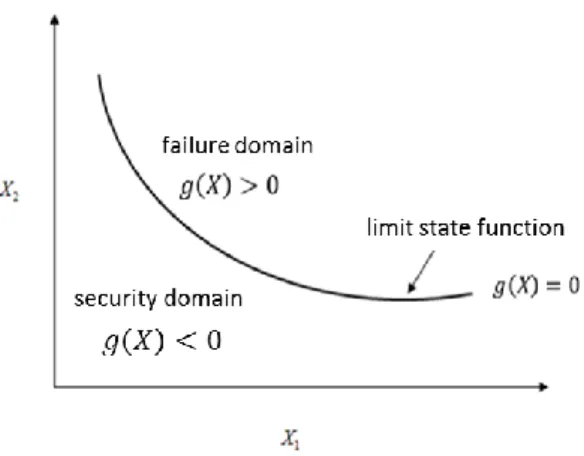
In the field of electromagnetic device manufacturing, the system ability to satisfy consumer’s demand or operating constraints is important. The reliability means that designers should reduce the probability of failure as much as possible. The determination of the reliability of the system is based on the limit state function. Each constraint 𝑔(𝑋) ≤ 0 can separate the domain of 𝑋 into three parts: the limit state curve is 𝑔(𝑋) = 0, the domain where 𝑔(𝑋) > 0 is the failure domain, on the contrary the security domain represents the area 𝑔(𝑋) < 0.

Figure 1. The failure domain, security domain, and limit-state curve.

The probability of failure is the probability of the event 𝑔(𝑋) > 0. It is calculated with the integral:

(4) 𝑃𝑓 = 𝑃[𝑔(𝑋) > 0] = 𝑃[𝑋 ∈ 𝐷𝑓] = ∫ 𝑓_𝐷 𝑋(𝑥)𝑑𝑥

𝑓

where 𝐷𝑓 is the failure domain. Because the computational burden is heavy with numerous random parameters,

direct integration is almost impossible and thus Monte-Carlo Simulation (MCS) or other techniques such as First-Order Reliability Method (FORM) [4], [5] is often used to calculate an approximation of 𝑃𝑓.

FORM and inverse FORM are based on an isoprobalistic transformation to have a normalized vector of statistically independent random variables 𝑈 instead of the initial input parameter 𝑋.

For the Gaussian vector 𝑋 in this paper, the transformation 𝑇 is as follows:

Figure 2. The first order reliability method [17].

Then the limit state function changes from 𝑔(𝑑) = 0 to 𝐺𝑈(𝑢) = 0 and the CDF from 𝐹𝑋 to 𝐹𝑈. 𝐺𝑈(𝑢) is

defined as the performance function, and the FORM or inverse FORM method uses a linear approximation to replace the real performance function at the Most Probable Point of failure (MPPF) in U-space. The MPPF 𝑢∗ _is

the one that minimize the distance between the origin 𝑂 and 𝐺𝑈(𝑢) = 0. After 𝑢∗ is found, the limit-state function

is replaced by a tangent hyperplane crossing 𝑢∗_{. So the probability of failure is calculated by:}

(6) 𝑃𝑓≈ ∫_𝐺̃ 𝑓𝑈(𝑢)𝑑𝑢 = 𝛷(−𝛽)

𝑈(𝑢)>0

where 𝐺̃𝑈(𝑢) = 0 is the hyperplane that approximates the limit-state function 𝐺𝑈(𝑢) = 0, 𝛷 is the standard

Gaussian cumulative distribution function, and 𝛽 = ‖𝑢‖ is the reliability index which is equal the norm of 𝑢. The formulation (2) is the basis of all RBDO methods and can be solved by different approaches which are usually separated in three main categories: double-loop, single-loop, and sequential decoupled methods. The following sections introduce the principle of these different categories and present some approaches for each of them.

2.2 Double-loop methods

Double-loop methods use two loops to solve RBDO problems: the inner loop aims to analyze reliability of the chosen configuration and to calculate the probability of failure using FORM or inverse FORM; the outer loop seeks the mean values of input designs that minimize the objective function and constrain the probability of failure computed by inner loop.

There are several approaches for double-loop methods, the most popular are Reliability Index Approach (RIA) and Performance Measure Approach (PMA) [3], [6].

2.2.1 Reliability Index Approach (RIA)

RIA uses the FORM to calculate the reliability index in the inner loop: (7)

𝛽 = min

𝑢 ‖𝑢‖

𝑠. 𝑡. 𝐺𝑈(𝑢) = 0

The outer loop of RIA, any constrained non-linear algorithm like SQP or others can be chosen to minimize the objective function 𝑓 with the index 𝛽 given by the FORM:

(8) min 𝑑 𝑓(𝑑) 𝑠. 𝑡. _{𝛽 ≥ 𝛽}𝑔 ≤ 0 𝑡 𝑑𝐿_{+ 𝛽} 𝑡∙ 𝜎 ≤ 𝑑 ≤ 𝑑𝑈− 𝛽𝑡∙ 𝜎

where 𝑔 < 0 is used to restrict the because the definition in equation (6) only validate if the origin is located in the security domain.

2.2.2 Performance Measure Approach (PMA)

In former formulation of RBDO, optimization is carried out with the limitation of the reliability index that must be greater than or be equal to a target value. The calculation of this index leads to the search for the MPPF. In contrast, for PMA formulation, optimization is formulated with the limitation of maximum performance with a given value of reliability index. The search of this maximum performance is to maximize the function 𝐺𝑈

with the limitation that reliability index must achieve the target value. This approach is considered as the inverse of the FORM approximation [7], [8].

So the outer loop becomes:

(9) min 𝑑 𝑓(𝑑) 𝑠. 𝑡. 𝐺𝑝(𝑢∗)

≤ 0

where 𝐺𝑝(𝑢∗) is the maximal performance measurement. The purpose of the inner loop is to find 𝑢∗ in U-space

such as: (10)

𝐺𝑝(𝑢∗) = max 𝑢 𝐺𝑈(𝑢)

𝑠. 𝑡. ‖𝑢‖ = 𝛽𝑡

where 𝑢∗ _{is the Maximum Performance Target Point (MPTP) that corresponds to the target index 𝛽} 𝑡.

2.3 Single-loop methods

For the so-called single-loop methods, the main point is that the inner loop is replaced by an approximation to avoid the iterative evaluations for reliability analysis in order to accelerate the convergence to the optimum.

2.3.1 Approximate Moment Approach (AMA)

AMA is based on statistical moments. The first order Taylor expansion is used to calculate the mean 𝜇𝑔_𝑖

and the standard deviation 𝜎𝑔_𝑖 for all constraint functions 𝑔𝑖(𝑑) by using the following expressions [9]:

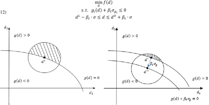
(11) { 𝜇𝑔𝑖= 𝑔𝑖(𝑑) 𝜎𝑔𝑖 2 _{≈ (}

_𝛻

∙

where 𝜎 is the standard deviation of the input variables 𝑋 and 𝛻 is the gradient operator. With these expressions, an approximation 𝑔𝑖(𝑑) + 𝛽𝑡𝜎𝑔_𝑖 is used to replace the original constraints 𝑔𝑖(𝑑′) as shown in Figure 3. In this way,

the margin of security is shifted in order to keep the reliability as desired. Figure 3 shows the basic idea of AMA approach, 𝑔(𝑑) = 0 is the deterministic limit-state function. As the optimum point 𝑑∗ _{is on the limit-state curve,}

the probability of failure is about 50%. The situation which could cause the failure around this point with a given probability is shown as shaded area on the left side. AMA transforms the constraint to find a new optimum point 𝑑′∗ _{on the curve of the new limit-state equation 𝑔(𝑑) + 𝛽}

𝑡𝜎𝑔= 0. The situation which could cause the failure

around 𝑑′∗ _{is greatly reduced as shown by the shaded area on the right side.}

So the problem becomes a deterministic problem:

(12) min 𝑑 𝑓(𝑑) 𝑠. 𝑡. 𝑔𝑖(𝑑) + 𝛽𝑡𝜎𝑔_𝑖 ≤ 0 𝑑𝐿_{− 𝛽} 𝑡∙ 𝜎 ≤ 𝑑 ≤ 𝑑𝑈+ 𝛽𝑡∙ 𝜎

This approach is based on a local linear approximation of the constraint functions at the mean value of the design parameters and as the probabilistic distribution of the performances depends on two moments that are also approximated, the reliability assessment could produce significant numerical error [10].

2.3.2 Single Loop Approach (SLA)

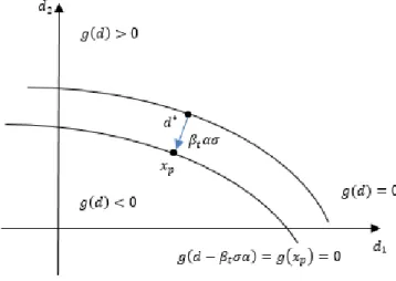
SLA uses the same approximation as AMA for calculating the moments and the position of MPPF (marked as 𝑑′∗ _{in Figure 3 and 𝑥}

𝑝 in Figure 4). The difference between these two methods is that SLA evaluates

the constraints 𝑔 at the approximate MPPF unlike AMA that uses a first-order approximation of the constraint function around the mean value 𝑑 directly. The formulation is given as [11]:

(13) min 𝑑 𝑓(𝑑) 𝑠. 𝑡. 𝑔_𝑖(𝑥_𝑝𝑖 )≤ 0 𝑑𝐿+ 𝛽_𝑡∙ 𝜎 ≤ 𝑑 ≤ 𝑑𝑈− 𝛽_𝑡∙ 𝜎 with (14) 𝑥_𝑝𝑖 = 𝑑 − 𝛽𝑡𝛼𝑖∘ 𝜎 𝛼𝑖= 𝛻𝐺_𝑈𝑖(𝑑) ‖𝛻𝐺_𝑈𝑖(𝑑)‖= 𝜎∘𝛻𝑔_𝑖(𝑑) ‖𝜎∘𝛻𝑔_𝑖(𝑑)‖

where 𝛼𝑖 is the normalized gradient of the 𝑖th constraint, 𝑥_𝑝𝑖 is the approximation of the MPPF for the constraint

𝑔𝑖 , and ∘ is the Hadamard operator (element-wise) product.

Figure 4. Principle of the SLA approach

The principle of this approach is similar to AMA. As shown in Figure 4, it does not search for the MPPF of each constraint by using an inner loop but approximate its position.

2.4 Sequential decoupled methods

Sequential decoupled methods aim to change the initial problem into a series of optimization cycles. The cycles are sequential, each individual optimization is deterministic and uses the optimum given by the former optimization as an initial point. At the first iteration, the algorithm searches a deterministic solution without considering uncertainty and then compute the reliability index of this solution to deduce a shift in order to achieve a given probability of failure. The next iterations refine the shift.

2.4.1 Sequential Optimization and Reliability Assessment (SORA)

SORA employs a series of cycles of deterministic optimizations and reliability assessments. In each cycle, optimization and reliability assessment are decoupled from each other, the reliability assessment is only conducted after the deterministic optimization to verify constraint feasibility under uncertainty. The main point of this method is to shift the boundaries of violated constraints to the feasible direction based on the reliability information obtained in the former cycle [12]. The updated point is used in the next cycle of the deterministic optimization. This cycle is repeated until the fulfillment of the convergence criteria.

The process of SORA method is presented as follows. First of all, an initial shift 𝑠0_{= 0 allows finding}

(15) 𝑑∗𝑘= argmin 𝑑𝑘 𝑓(𝑑 𝑘₎ 𝑠. 𝑡. 𝑔(𝑑𝑘_{− 𝑠}𝑘_{) ≤ 0} 𝑑𝐿+ 𝛽_𝑡∙ 𝜎 ≤ 𝑑 ≤ 𝑑𝑈− 𝛽_𝑡∙ 𝜎

where 𝑘 indicates the iteration number. The optimal value is set as 𝑑∗𝑘_{. After each optimization, some of the}

constraints may become active. For an active constraint, the optimal point 𝑑∗𝑘 _{is on the limit-state curve. When}

considering the randomness of 𝑋, the actual probability of failure is about 0.5, so a reliability assessment is implemented at the deterministic optimum solution to locate the MPTP 𝑥𝑘 _{that corresponds to the desired}

probability of failure. To ensure the MPTP onto the deterministic boundary, a shifting vector 𝑠𝑘+1 _{is derived:}

(16) 𝑠𝑘+1= 𝑑∗𝑘− 𝑥𝑘

Therefore, when establishing the equivalent deterministic optimization model in the next cycle, the constraints is modified to shift the MPTP at least onto the deterministic boundary.

2.4.2 Sequential Approximate Programming (SAP)

SAP is another approach based on Taylor expansion at the first order. The original optimization problem is decomposed into a sequence of sub-optimization problems. Each sub-optimization consists of an approximate objective function subjected to a set of approximate constraint functions [13]. The details are presented as follows: For considering the PMA formed optimization problems, the expressions are as equation (8), following the idea of SAP, a sequential approximate formulation is constructed as:

(17) min 𝑑 𝑓 𝑘_(𝑑) 𝑠. 𝑡. 𝐺𝑝(𝑑𝑘) ≤ 0 𝑑𝐿_{+ 𝛽} 𝑡∙ 𝜎 ≤ 𝑑 ≤ 𝑑𝑈− 𝛽𝑡∙ 𝜎

The approximate function 𝐺𝑝(𝑑𝑘) is built with a first order Taylor expansion with respect to the design

variables at the current point:

(18) 𝐺𝑝(𝑑𝑘) ≈ 𝐺̂𝑝(𝑑𝑘−1) + (𝛻𝑑𝐺̂𝑝(𝑑𝑘−1)) 𝑇

(𝑑𝑘_{− 𝑑}𝑘−1₎

where 𝐺̂𝑝(𝑑𝑘−1) = 𝐺𝑢(𝑢𝑘−1) is the approximate probabilistic performance measure and 𝛻𝑑𝐺̂𝑝(𝑑𝑘−1) is its

gradient. To avoid another optimization to calculate 𝑢𝑘_{, it is updated by the function below:}

(19) 𝑢𝑘_{= −𝛽}

𝑡

𝛻𝑈𝐺𝑈(𝑢𝑘−1) ‖𝛻_𝑈𝐺_𝑈(𝑢𝑘−1_)‖

where 𝑢0_{= 0 is usually chosen as the initial estimation.}

With the first order approximation of 𝐺𝑝(𝑑𝑘), new formulation is obtained:

(20) min 𝑑 𝑓 𝑘_(𝑑) 𝑠. 𝑡. 𝐺̂𝑝(𝑑𝑘−1) + (𝛻𝑑𝐺̂𝑝(𝑑𝑘−1)) 𝑇 (𝑑 − 𝑑𝑘−1_{) ≤ 0} 𝑑𝐿_{+ 𝛽} 𝑡∙ 𝜎 ≤ 𝑑 ≤ 𝑑𝑈− 𝛽𝑡∙ 𝜎

This formulation of SAP is similar to the outer loop of PMA. The same principle is used to convert a RIA formulation into a sequential approximate programming [14].

3 CASE STUDIES

In this chapter, two examples are tested to compare the performances of all approaches.

3.1 Numerical example

To assess the efficiency of these methods, the simple two-variable problem in [15] is analyzed. The optimization problem of this numerical example is:

(21) min 𝑑 𝑓(𝑑) = − (𝑑1+𝑑2−10) 2 30 − (𝑑1−𝑑2+10) 2 120 𝑠. 𝑡. { 𝑔1= 1 − 𝑑₁2𝑑₂ 5 𝑔2= 1 − (𝑑1+𝑑2−5)2 30 − (𝑑1−𝑑2−12)2 120 𝑔3= 1 − 80 (𝑑₁2+8𝑑₂+5) 0 ≤ 𝑑1,2 ≤ 10

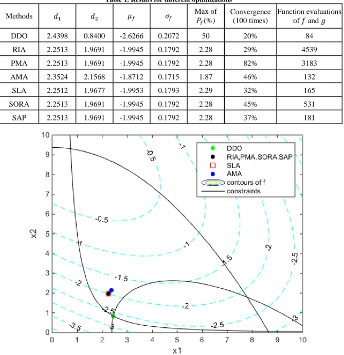
In order to understand the implications of the choice of different formulations and also to quantify the impact of the choice of approaches and algorithms on the accuracy and the number of evaluations, the results of the 7 mentioned methods are given in Table 1. The different optima are compared with each other in Figure 5, where the dotted curves present contours of 𝑓 and constraint boundaries 𝑔𝑖= 0 are depicted as solid lines. The

target probability of failure 𝑃𝑡 for RBDO is 2.28%, 𝑃𝑓 is computed by Monte-Carlo simulation with a sampling

of 106 _{realizations. For the simplicity and without loss of generality, all the uncertainties are modeled with the}

normal law.

Table 1. Results for different optimizations

Methods 𝑑1 𝑑2 𝜇𝑓 𝜎𝑓 Max of 𝑃𝑓(%) Convergence (100 times) Function evaluations of 𝑓 and 𝑔 DDO 2.4398 0.8400 -2.6266 0.2072 50 20% 84 RIA 2.2513 1.9691 -1.9945 0.1792 2.28 29% 4539 PMA 2.2513 1.9691 -1.9945 0.1792 2.28 82% 3183 AMA 2.3524 2.1568 -1.8712 0.1715 1.87 46% 132 SLA 2.2512 1.9677 -1.9953 0.1793 2.29 32% 165 SORA 2.2513 1.9691 -1.9945 0.1792 2.28 45% 531 SAP 2.2513 1.9691 -1.9945 0.1792 2.28 37% 181

The column named convergence in Table 1 means that we run the algorithms 100 times with different initial points to see how many times it converges to the same optimum. From Table 1 and Figure 5, we can see that most of the methods can find a result that satisfies the constraints. DDO leads to a solution with the lowest objective function mean value, the highest standard-deviation of objective function and a probability of failure around 50%. On the contrary, the probabilities of failure of RBDO methods are close to the target probability except for the single-loop method AMA because of the approximation used to increase the speed of convergence by sacrificing the accuracy. Among RBDO methods, single-loop strategies are fast but inaccurate, double-loop and sequential decoupled methods lead to the same results but sequential decoupled methods are greatly faster.

3.2 Example of safety transformer optimization

The example of a safety isolating transformer [16] is also investigated. This is a single-phase transformer with grain-oriented E-I laminations. The primary and secondary windings are both wound around the frame surrounding the central core. The model inputs consist in 7 random design parameters: three parameters 𝑎, 𝑏, 𝑐 for the shape of the lamination, one for the frame 𝑑, two for the section of conductors 𝑆1, 𝑆2 and the last one for the

number of primary turns 𝑛1. These design variables are shown in Figure 6. The range of input variables are:

(22) 3𝑚𝑚 ≤ 𝑎 ≤ 30𝑚𝑚 14𝑚𝑚 ≤ 𝑏 ≤ 95𝑚𝑚 6𝑚𝑚 ≤ 𝑐 ≤ 40𝑚𝑚 10𝑚𝑚 ≤ 𝑑 ≤ 80𝑚𝑚 200 ≤ 𝑛1≤ 1200 0.15𝑚𝑚2_{≤ 𝑆} 1≤ 19𝑚𝑚2 0.15𝑚𝑚2_{≤ 𝑆} 2≤ 19𝑚𝑚2

There are 8 inequality constraints in this problem. The copper and iron temperatures 𝑇𝑐𝑜𝑛𝑑 and 𝑇𝑖𝑟𝑜𝑛

should be less than given temperatures 120℃ and 100℃ respectively. Both the magnetizing current 𝐼10

𝐼1 and drop

voltage ∆𝑉2

𝑉₂₀ should be less than 10%. The filling factors of the primary coil 𝑓1 and secondary coil 𝑓2 should be

lower than 1, and the efficiency 𝜂 should be larger than 0.8. At last, the residue must be less than 10−6_.

The constraint functions are:

(23) 𝑔(𝑑) = [ 𝑇𝑐𝑜𝑛𝑑− 120 𝑇𝑖𝑟𝑜𝑛− 100 𝐼10⁄𝐼1− 0.1 ∆𝑉2⁄𝑉20− 0.1 𝑓1− 1 𝑓2− 1 0.8 − 𝜂 𝑟𝑒𝑠𝑖𝑑𝑢𝑒 − 10−6_]

The aim is to minimize the total mass 𝑀𝑡𝑜𝑡 with a target probability 𝑃𝑡= 0.13%, so that the target

reliability index is 𝛽𝑡= 3.

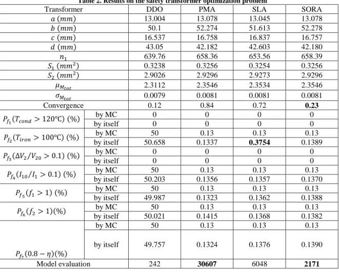
Table 2 shows the results of some methods. For each constraint, there are two probabilities of failures, upper ones are calculated by the methods themselves and the below ones are calculated by the Monte-Carlo simulation for comparison. For the reason that the 8th _{constraint is a residue, we consider it as a deterministic one,}

so there are only 7 probabilities of constraints presented in the table 2.

Table 2. Results on the safety transformer optimization problem

Transformer DDO PMA SLA SORA

𝑎 (𝑚𝑚) 13.004 13.078 13.045 13.078 𝑏 (𝑚𝑚) 50.1 52.274 51.613 52.278 𝑐 (𝑚𝑚) 16.537 16.758 16.837 16.757 𝑑 (𝑚𝑚) 43.05 42.182 42.603 42.180 𝑛1 639.76 658.36 653.56 658.39 𝑆1 (𝑚𝑚2_{) 0.3238 0.3256 0.3254 0.3256} 𝑆2 (𝑚𝑚2_{) 2.9026 2.9296 2.9273 2.9296} 𝜇𝑀𝑡𝑜𝑡 2.3112 2.3546 2.3534 2.3546 𝜎𝑀𝑡𝑜𝑡 0.0079 0.0081 0.0081 0.0081 Convergence 0.12 0.84 0.72 0.23 𝑃𝑓₁(𝑇𝑐𝑜𝑛𝑑> 120℃) (%) by MC 0 0 0 0 by itself 0 0 0 0 𝑃𝑓₂(𝑇𝑖𝑟𝑜𝑛> 100℃) (%) by MC 50 0.13 0.13 0.13 by itself 50.658 0.1337 0.3754 0.1389 𝑃𝑓₃(∆𝑉2⁄𝑉20> 0.1) (%) by MC 0 0 0 0 by itself 0 0 0 0 𝑃𝑓₄(𝐼10⁄𝐼1> 0.1) (%) by MC 50 0.13 0.13 0.13 by itself 50.203 0.1356 0.1357 0.1370 𝑃𝑓₅(𝑓1> 1) (%) by MC 50 0.13 0.13 0.13 by itself 49.987 0.1323 0.1362 0.1388 𝑃𝑓₆(𝑓2> 1)(%) by MC 50 0.13 0.13 0.13 by itself 50.021 0.1415 0.1368 0.1382 𝑃𝑓₇(0.8 − 𝜂)(%) by MC 50 0.13 0.13 0.13 by itself 49.757 0.1324 0.1376 0.1390 Model evaluation 242 30607 6048 2171

Note that PMA can find an optimum that satisfies all the constraints even if the number of evaluations of the model is high. For SLA, it has a smaller number of evaluations but there is one constraint violated. The reason is that SLA sacrifices the accuracy in order to reduce the number of evaluations, leading to a coarse computation of the probability of failure. The convergence rate of SORA is not as good as the other two but it has the smallest number of evaluations among them. It can be seen that this number is nearly 15 times less than PMA and 3 times less than SLA. Unfortunately, the rate of convergence for SORA is 4 times lower. This means that a multi-start process is required and the number of evaluations will increase consequently. We obtain almost the same conclusions as with the numerical example: the single-loop method SLA is the most inaccurate method and double-loop method PMA has the highest convergence rate. For this more complicated example, the number of evaluations of sequential decoupled method SORA is even smaller than of SLA, so that the more complex the model is, the more effective SORA may be. Other methods fail to find a solution, probably because this problem is hard-constrained and the solution of DDO is on the limit-state of four constraints. So, it also indicates that not all the aforementioned approaches can handle complicated models.

4 CONCLUSION

RBDO methods change the initial constraints into probabilistic ones and use different approaches to approximate the limit state function or the most probable point of failure to calculate the probability of failure or the reliability index.

The mathematical example shows that the 6 RBDO approaches have almost the same results except AMA that is less accurate. The optimization of the safety transformer highlights that not all the methods can converge to

the global solution. PMA, SLA, and SORA appear to be more stable. Considering both numerical examples, SORA is the most effective method among all RBDO approaches.

REFERENCES

[1] Xiao, S., Li, Y., Rotaru, M., Sykulski, J. K. (2014), "Considerations of uncertainty in robust optimisation of electromagnetic devices",

International Journal of Applied Electromagnetics and Mechanics, Vol. 46 No. 2, pp. 427-436.

[2] Kim, D. W., Kang, B., Choi, K. K., et al. (2016), "A Comparative Study on Probabilistic Optimization Methods for Electromagnetic

Design", IEEE Transactions on Magnetics, Vol. 52 No. 3, pp. 1-4.

[3] Ren, Z., Zhang, D., and Koh, C. S. (2016). "Investigation of reliability analysis algorithms for effective reliability-based optimal design of electromagnetic devices", IET Science, Measurement & Technology, Vol. 10 No. 1, pp. 44-49.

[4] Liu, P.L., Der Kiureghian, A. (1991), "Optimization algorithms for structural reliability", Structural safety, Vol. 9 No. 3, 1991, pp. 161-177.

[5] Hasofer, A.M. and Lind, N.C. (1974), "Exact and invariant second-moment code format. American Society of Civil Engineers",

Engineering Mechanics Division, Vol. 100, pp. 111-121.

[6] Tu, J., Choi, K.K., and Park, Y.H. (1999), "A new study on reliability-based design optimization", Journal of mechanical design, Vol.

121 No. 4, pp. 557-564.

[7] Wu, Y.T., Millwater, H.R., Cruse, T.A. (1990), "Advanced probabilistic structural analysis method for implicit performance functions",

AIAA journal, Vol. 28 No. 9, pp. 1663-1669.

[8] Youn, B.D., Choi, K.K. and Park, Y.H. (2003), "Hybrid analysis method for reliability-based design optimization", Journal of

Mechanical Design, Vol. 125 No.2, pp. 221-232.

[9] Putko, M.M, Taylor, A.C., Newman, P.A., et al. (2002), "Approach for input uncertainty propagation and robust design in CFD using

sensitivity derivatives", Journal of Fluids Engineering, Vol. 124 No. 1, pp. 60-69.

[10] Youn, B.D., and Choi, K.K. (2004), "Selecting probabilistic approaches for reliability-based design optimization", AIAA journal, Vol. 42 No. 1, pp. 124-131.

[11] Liang, J., Mourelatos, Z.P., and Tu, J (2004), "A single-loop method for reliability-based design optimization", in ASME 2004

International Design Engineering Technical Conferences and Computers and Information in Engineering Conference, 2004, Salt Lake

City, pp. 419-430.

[12] Du, X., and Chen, W. (2004), "Sequential optimization and reliability assessment method for efficient probabilistic design)", Journal of

Mechanical Design, Vol. 126 No. 2, pp. 225-233.

[13] Yi, P., Cheng, G., and Jiang, L. (2008), "A sequential approximate programming strategy for performance-measure-based probabilistic structural design optimization", Structural Safety, Vol. 30 No. 2, pp. 91-109.

[14] Cheng, G., Xu, L., and Jiang, L. (2006), "A sequential approximate programming strategy for reliability-based structural optimization",

Computers & structures, Vol. 84 No.21, pp. 1353-1367.

[15] Kim, D.W., Choi, N.S., Choi, K.K. et al. (2015), "A Single-Loop Strategy for Efficient Reliability-Based Electromagnetic Design Optimization", IEEE Transactions on Magnetics, Vol. 51 No. 3, pp. 1-4.

[16] Tran, T.V., Brisset, S. and Brochet, P. (2007), "A Benchmark for Multi-Objective, Multi-Level and Combinatorial Optimizations of a Safety Isolating Transformer", in 16th International Conference on Computation of Electromagnetic Fields, 2007, Aachen, pp. 167-168. [17] Lopez, R.H. and Beck, A.T. (2012), "Reliability-based design optimization strategies based on FORM: a review", Journal of the