• Aucun résultat trouvé

Importance of suppression and mitigation measures in managing COVID-19 outbreaks

N/A
N/A
Protected

Academic year: 2021

Partager "Importance of suppression and mitigation measures in managing COVID-19 outbreaks"

Copied!
16
0
0

Texte intégral

(1)

HAL Id: hal-03018341

https://hal.archives-ouvertes.fr/hal-03018341

Preprint submitted on 22 Nov 2020

HAL is a multi-disciplinary open access archive for the deposit and dissemination of sci-entific research documents, whether they are pub-lished or not. The documents may come from teaching and research institutions in France or abroad, or from public or private research centers.

L’archive ouverte pluridisciplinaire HAL, est destinée au dépôt et à la diffusion de documents scientifiques de niveau recherche, publiés ou non, émanant des établissements d’enseignement et de recherche français ou étrangers, des laboratoires publics ou privés.

Michael Hochberg

To cite this version:

Michael Hochberg. Importance of suppression and mitigation measures in managing COVID-19 out-breaks. 2020. �hal-03018341�

(2)

Importance of suppression and mitigation measures in managing COVID-19

outbreaks

Michael E. Hochberg

ISEM, University of Montpellier, CNRS, IRD, EPHE, Montpellier, France Santa Fe Institute, Santa Fe, New Mexico, USA

michael.hochberg@umontpellier.fr

Abstract

I employ a simple mathematical model of an epidemic process to evaluate how four basic quantities: the reproduction number (ℛ), the numbers of sensitive (S) and infectious individuals (I), and total community size (N) affect strategies to control COVID-19. Numerical simulations show that strict suppression measures at the beginning of an epidemic can create low infectious numbers, which thereafter can be managed by mitigation measures over longer periods to flatten the epidemic curve. The stronger the suppression measure, the faster it achieves the low numbers of infections that are conducive to subsequent management. Our results on short-term strategies point to a two-step control strategy, following failed mitigation, that begins with suppression of the reproduction number, ℛC, below 1.0, followed by renewed mitigation measures that manage

the epidemic by maintaining the effective reproduction number ℛCeff ≈ ℛCS/N at approximately

1.0. The objectives of the full sequence of measures observed in a number of countries, and likely to be seen in the longer term, can be symbolically represented as: ℛ0 à ℛC<ℛ0 à ℛC<1.0 à

Ceff≈1.0. We discuss the predictions of this analysis and how it fits into longer-term sequences

of measures, including misconceptions about ‘flattening the curve’ and how the herd immunity concept can be used to ‘leverage’ immunity.

(3)

Introduction

The COVID-19 pandemic is a major global threat. Spread of the SARS-CoV-2 virus began in China in late 2019, with 41 cases recorded according to the WHO as of January 11/12, 2020, attaining more than 25 million confirmed cases worldwide as of September 1st (1). By its highly

transmissible and virulent nature, COVID-19 is putting considerable strain on health services, meaning that increasing numbers of patients in the most afflicted countries cannot be adequately cared for, which will likely further exacerbate disease morbidity and mortality.

Research groups have mobilized to collect and analyze molecular (2) and epidemiological (3-5) data, and employ statistical and mathematical models to simulate regional and national outbreaks and the global pandemic, and evaluate possible control measures (e.g., 6-14).

Particularly important in this effort is the projection of how different strategies will affect outbreaks. Conducting such studies without delay is crucial, both because most countries are in early outbreak stages and thus open to management options, and since some nations are days or even weeks behind in their epidemics compared to others. The latter property is important, since the lockstep nature of COVID-19 epidemic trends mean that nations can ‘peer into the future’ to predict how their own outbreaks could unfold. This information and the efficacy of control strategies already adopted by other ‘future’ countries can be instrumental in giving the time needed to plan and logistically organize effective measures.

Here, we employ a simple epidemiological model to elucidate some of the basic parameters and processes that arbitrate short-term control measure outcomes. The model’s intuitive results emphasize the necessity to adopt one or both of two strategies. ‘Suppression measures’ are engaged early and decisively to lower the reproduction number, ℛ, below 1.0 and as close as feasible to 0.0. When successful, this results in low, manageable numbers of infections (a low ‘set-point’), and can then be followed by a second strategy: ‘Mitigation measures’ that continue to flatten the epidemic curve by maintaining the reproduction number to approximately 1.0. However, strategies need not follow this sequence. For those countries reacting very early in an outbreak, mitigation measures alone may be sufficient. For those that are late and/or unable to employ radical suppression measures, ‘progressive mitigation’ so as to lower ℛ below 1.0 may be the only alternative.

The objective of the present study is to emphasize how strategic lowering of the reproduction number is central to a rational management plan to minimize the impacts of COVID-19. Because local outbreaks are producing large numbers of recovered cases, this opens the possibility that any acquired immunity can be ‘leveraged’ to reduce the intensity of future policies.

(4)

Model

We employ a modified SEIR model of Susceptible (S) → Exposed (E) → Infectious (I) → Removed (R) states (15). The ordinary differential equations take the form:

𝑑𝑆 𝑑𝑡 = −b 𝐼𝑆 𝑁 𝑑𝐸 𝑑𝑡 = b 𝐼𝑆 𝑁 − 1 𝑇./0 𝐸 𝑑𝐼 𝑑𝑡= 1 𝑇./0 𝐸 − 𝛾𝐼 𝑑𝑅 𝑑𝑡 = 𝛾𝐼,

where N is a constant equal to S+E+I+R, b is the transmission parameter, Tinc is the incubation period, 𝛾 is the rate of removal into different subclasses of R. Specifically, R is composed of minor cases 𝐶5, severe cases at home 𝐶6, severe cases in hospital 𝐶78, and fatalities 𝐶9, given by

𝑑𝐶5 𝑑𝑡 = 𝑃5 𝛾 𝐼 − 𝐶5 𝐷<5 , 𝑑𝐶7 𝑑𝑡 = 𝑃7 𝛾 𝐼 − 𝐶7 𝐷8= , 𝑑𝐶78 𝑑𝑡 = 𝐶7 𝐷8= − 𝐶78 𝐷<7 , 𝑑𝐶9 𝑑𝑡 = 𝑃9 𝛾 𝐼 − 𝐶9 𝐷9 .

Here, 𝑃5 , 𝑃7 , and 𝑃9 are, respectively, the probabilities of a case being mild, severe and resulting in death (𝑃5 + 𝑃7 + 𝑃9 = 1). 𝐷<5, 𝐷<7, 𝐷8=, are days to recovery for mild and severe cases, time of hospitalization, and 𝐷9 is the time from end of incubation to death (Titod) minus duration of infectiousness (Tinf).

An outbreak occurs if the basic reproduction number, ℛ0 = b / 𝛾 > 1.0. The impact of control

measures is easily understood by their impact on ℛ0, and in the presentation below, we refer to

(5)

Numerical methods

We employ this general model for COVID-19 to explore how some of its central properties could affect outbreak control efforts. The over-simplicity of the model means that it should not be used to make precise predictions for actual epidemic management situations, but rather serve as a conceptual tool that can serve as a first step towards more realistic analyses for specific scenarios or situations.

Specifically, we focus on how two generic types of objective – suppression and mitigation – affect epidemiological and clinical parameters. We expect that, all else being equal, suppression will reduce ℛ0 more than would mitigation. However, their impacts on ℛ0 are expected to differ from

locality to locality depending on the details of (and adherence to) the measures deployed. This argues for examining a range of ℛC for each of the two types of objective,and recognizing that

mitigation measures in one locality (e.g., country) could be more effective at lowering ℛ0 than

suppression measures in another.

Epidemic management strategies were investigated using the Epidemic Calculator package (16) (Supplementary Material). This platform is rich in possibilities for varying key parameters such as the reproduction number (ℛ) and temporal scales of infection (Tinf and Tinc), as well as initial

sub-population of infections individuals (I0) and the total population size (N=S0+I0). The platform

also permits the user to experiment with different “clinical” parameters, including hospitalization rate, case fatality rate, and recovery time for mild cases.

The results presented below are based on the parameter values provided on the website simulator page (Table 1). Given the recent emergence of COVID-19, these parameter values should be viewed as preliminary and possibly inaccurate, since for example, they may be based on limited data or be time- or location-specific. This reinforces the above call for caution in interpreting the findings presented here, and in using the precise model output for any specific management actions.

Parameter Value

Basic Reproduction Number (ℛ0) 2.5,3.0

Infectious period (Tinf) 2.9 days

Removal rate (g ) 1.0/Tinf

(6)

Case fatality rate (𝑃9 ) 0.02 Time from end of incubation to death (Titod) 32 days

Recovery time for severe cases (𝐷<7) 28.6 days Recovery time for mild cases (𝐷<5) 11.1 days

Hospitalization rate (𝑃7 ) 0.2 Time to hospitalization (𝐷8=) 5 days

Table 1. Parameters and their baseline values employed in this study. ℛ0 values investigated are based on (3,6). See

(16) for details on other parameters.

The Epidemic Calculator package, although very flexible, has some limitations in its use for scientific study. First, the accuracy of the simulator output is untested with respect to analytical results, independent computational studies, and other SEIR platforms. The only test conducted here did verifiy that the simulated equilibrium fraction of susceptible individuals (S¥) followed

the predicted relation: -ln(S¥/S0)= ℛ(1-S¥/S0) (15). The results presented below – even if

consistent with intuition – nevertheless need to be viewed as preliminary and contingent on future testing. Second, precision in the intervals for input parameters and platform output were not always to the last decimal places, and for large numbers, such as the total community size N, a limited number of choices were available. Therefore, for example, there was no choice for exactly N=70 million, and as such the next highest option (70,420,854) was employed. The same was true for simulations with the lower population size of N=70K (70,263 was used). Moreover, the data presented below (i.e., y-axis data point readings) were in some cases closest interpolations of closely neighboring values that resulted in the simulation target. Varying the input and reading rules to neighboring values was found to have negligible effects on the trends reported, and did not change the main conclusions of this study.

Results

We first explored how the trigger number of infectious cases (I) for suppression measures to be engaged, affected the critical level of ℛC necessary to keep infectious cases at or below a set-point

of 100 after 60 days. We chose 60 days because it is the approximate period that areas of China (as the first affected country), decided to enter lockdown.

(7)

Figure 1. Suppression levels required to meet objectives, given different starting conditions. Simulations begin with no measure imposed (ℛ0=2.5) and 1 infectious individual in a population of c. 70 million unexposed individuals. The

suppression strategy starts when the number of infectious individuals attain a given number (x axis), which correlates with the time elapsed in the outbreak. ℛC is the observed maximum level of ℛ needed to result in a set-point of 100

or fewer infectious individuals after 60 days of confinement (y – axis). Although not shown, imposing mitigation measures in the range 1.0<ℛC<2.5 prior to suppression does not change this basic result. Lines linking points aid

visualization. See text for further details.

Figure 1 shows that larger numbers of infectious individuals require stricter measures to attain

the (arbitrary) set-point objective of 100 or fewer circulating infectious individuals after two months of measures. According to our simulations, a population the approximate size of Western European nations such as France, Spain, the UK and Germany would need to reduce transmission probabilities to near zero to attain the objective, should infectious numbers be on the order of 100,000. Early interventions in populations with 1 to 100 circulating infectious individuals would still require considerable measures, with reductions in baseline ℛ0=2.5 of 25% to 60%,

respectively. Given cumulative case number doubling times observed in some countries of about 3 to 5 days (17) (and therefore c. 2 weeks between each log integer on the x-axis of Figure 1), the choice of measures without knowing their true impacts on the reproduction number could have resulted in insufficient flattening of the epidemic curve and valuable time lost. The data in Table

2 support these insights, whereby suppression measures need to be increasingly strict in order to

reduce the time necessary to obtain low target case numbers.

Duration (days) ℛC=0.1 E,I ℛC=0.5 E,I ℛC=0.9 E,I 0 11643,4645 11643,4645 11643,4645 10 2392,2261 5240,3643 9480,5475

(8)

20 492,500 2563,1801 8339,4829

30 102,105 1257,884 7340,4251

40 21,22 617,434 6460,3741

50 4,5 303,213 5684,3292

60 1,1 148,104 5000,2896

Table 2. Effect of suppression measure intensity and duration on the number of cases in incubation (E) and infectious (I) stages. N=70,420,854. ℛ0=2.5. Start day of intervention=64. E64=11,643, I64=4,645.

We then asked how population size and the effectiveness of suppression measures would condition how subsequent mitigation measures attain objectives after 200 days. We conducted a 2 x 2 numerical experiment. The first variable was community size, taken either to be a small city of about 70,000 inhabitants or a medium-sized nation of about 70 million. (Additional numerical experiments not presented here indicate that the observed trends apply at least in the total population range of 104 to 108). The second variable explored was the effectiveness of previous

suppression measures; we evaluated high effectiveness (a reset to a single infectious case) and a less, but still acceptable reset to 100 infectious cases. Clearly, any subsequent mitigation measures yielding ℛC<1.0 would result in infectious cases decreasing over time (and therefore be a

successful outcome), but given the impacts of such measures on society, below we consider strategies that seek to contain a second epidemic by tuning ℛC to between 1.0 and ℛ0.

Figure 2 shows how the effectiveness of suppression strategies and community size influence

how subsequent mitigation measures affect epidemiological and clinical parameters. For example, regulating the infectious numbers to less than 10% of the total population requires ℛC less than

c.1.5, which is about a 40% reduction in the ℛ0 assumed here (Fig. 2A). Peak levels of

hospitalization can reach c.7%-10% should mitigation measures be 20% or less effective at reducing ℛ0 (Fig. 2B). Such levels would exceed hospital bed capacity in most countries by at

least an order of magnitude (18). Reducing peak hospitalization levels well below 1% (which is still too high for many health services) would require ℛC close to 1.0. Finally, similar to the trends

in Figs. 2A,B, fatalities are sensitive to the effectiveness of prior suppression measures and community size, indicating that ℛC needs to be reduced towards unity for smaller communities

and those unable to reduce infectious cases sufficiently during suppression measures (Fig. 2C). These results emphasize that epidemics could be contained by tuning ℛC close to, but above 1.0,

(9)

Figure 2. Effect of mitigation ℛC on (A) The fraction of

initially unexposed people who are eventually exposed (Et+It+Rt) at t=200 days after

the measure starts; (B) The maximum daily fraction of the population needing hospitalization for any single day, up to 200 days after the measure starts; (C) The fraction of initially unexposed people who die during the 200 days of outbreak mitigation. Lines linking points aid visualization. Mitigation starts at: Yellow line, I0=1, N=70 million; Gray

line: I0=100, N=70 million; Red

line: I0=1, N=70K; Black line:

I0=100, N=70K. ℛ0=2.5.

Although not explored here, numerical simulations for parameter values associated with points above the dashed line in (A) were influenced by ‘herd immunity’, i.e., when the proportion of the population that is immunized exceeds (1.0-1.0/ℛ) (19). Moreover, note that the result in (A) appears to contrast with the results in Steir et al. (5), who showed higher case growth rates with city size. The discrepancy can be explained by the different units employed in each study (case growth rate in (5) vs. fraction of total population infected at some point during a fixed time interval (this study)) and how ℛ was estimated in (5) (found to be city-size dependent) vs. assumed invariant in the present study. Case growth rate (number of new cases on day t – number of new cases on day t-1 / number of new cases on day t-1) was found to increase with community size in the present study (not shown). Numbers above points in (B) refer to the day that maximum hospitalization occurs, and are only shown for the Black line conditions (note that when ℛC=1.0, maximum levels begin

on day 90 and are constant thereafter; for ℛC=1.1,

maximum levels occur after 200 days). See main text for additional details.

(10)

The herd immunity threshold is contingent on ℛ0. But policies that reduce transmissions resulting

in ℛ < ℛ0 will reduce the threshold. We observed that the attainment of herd immunity, whereby

the total immunized fraction of the population exceeds (1.0-1.0/ℛ), did not ensure the rapid end to an outbreak (Fig. 2A). Indeed, ‘epidemic overshoot’ (20) occurs in this simple model for all ℛ>1.0. Figure 3 extends the findings in Fig. 2A (limited to 200 days) to different points in the epidemic. We see that infected levels exceed the herd immunity threshold (black line) before maximum hospitalizations are observed (gray line). For ℛC≥1.2 the overshoot by the end of the

epidemic (blue line) is between c.15-30% of the population. Moderate levels of mitigation can have major impacts in the short term (cf. ℛC=2.0 vs. ℛ0=3.0 at 60 days), but as the epidemic runs

its course, the sensitivity of ℛC exceeding 1.0 becomes apparent; for example, ℛC=1.2 results in

c.30% of the population infected at some point during the epidemic. We discuss the implications

of this important finding for policies that ‘leverage’ immunity in the Conclusions.

Figure 3. Epidemic overshoot: Effect of mitigation ℛC on the total percentage of an initially susceptible population

infected by the virus at different points in the epidemic. I0=100, N=70 million. Red line = 60 days after 100th infectious

case; Black line = herd immunity threshold, expressed as the fraction of the initial population eventually infected; Gray line = day of peak hospitalizations (numbers indicate day); Blue line = end of epidemic. Note as in Figure 2A, the herd immunity threshold is contingent on ℛ. ℛ0 =2.5, 3.0 is shown for comparison. Lines linking points aid

visualization. See main text for additional details.

Finally, whereas mitigation measures result in fewer cases (Figs. 2, 3), if ℛC>1.0, then they also

lengthen the course of the epidemic (Figure 4). An epidemic with no mitigation (example shown

% Infected

0 10 20 30 40 50 60 70 80 90 100 ℛC=1.5 ℛC=2.0 ℛ0=2.5 ℛ0=3.0 ℛC=1.0 79 124 199 380 110

(11)

closest to the mitigation target of a flat epidemic (ℛC =1.2) is 80% complete after 482 days and

95% at 585 days. The implications of long-term mitigation levels are discussed below.

Figure 4. Effect of mitigation ℛC on the number of days until 80%=blue, 90%=orange, or 95%=gray of eventual

infections occur, during the full course of an epidemic. I0=100, N=70 million. ℛ0 =3.0 is shown for comparison See

main text for additional details.

Conclusions and future directions

The lockstep nature of COVID-19 outbreaks in different regions, countries and cities means that management practices in places further along the epidemic curve can inform those in earlier stages. Control strategies in one country, however, are not always applicable in others, due for example to cultural and logistical differences (21). Mathematical models based on empirical data have a role to play in adapting capacities to address epidemics, both as conceptual aids and management tools. The present study explored two generic types of intervention that can contribute to reducing the impact of COVID-19 epidemics. ‘Suppression measures’ would be adopted by communities that either initially decided not (or did, but were unable) to mitigate the exponential increase of new cases. Suppression reduces the reproduction number below 1.0, and in so doing lowers the number of infectious cases to a manageable level. ‘Mitigation measures’ may either be introduced as a preventive approach, whereby communities begin to manage very early in an outbreak, gradually introduced towards the end of a suppression strategy, or for countries unable or unwilling to enforce suppression measures, the only route possible to flatten

Days after

100

th

case

0 100 200 300 400 500 600 ℛC=1.2 ℛC=1.5 ℛC=2.0 ℛ0=3.0

(12)

the epidemic curve. The sequence of objectives observed in a number of countries, and likely to be seen in future months, can be symbolically represented as sequential stages:

𝓡0 à 𝓡C<𝓡0 à 𝓡C<1.0 à 𝓡Ceff≈1.0

The latter condition (ℛCeff ≈ 1.0) was not explored in this study, but ‘leverages’ any acquired

immunity so as to maintain the effective reproduction number ℛCeff ≈ ℛCS/N near 1.0 (see

discussion below).

The actual application of measures to meet this sequence of objectives is likely to be complex

(12-14), and in particular, mitigation measures could go through multiple successive adjustments in

the latter two phases represented above.

Our analysis presented here yield a number of important insights and predictions:

1. The number of infectious cases at the start of suppression determine how effective these

measures are at creating a reset. Communities with more than 100,000 infectious cases

essentially have to reduce transmission to zero in order to have about 100 cases after 60 days. Greater suppression measure stringency also means that with slightly longer confinement periods, an ever-lower set-point in the numbers of infectious individuals can be obtained. This permits reduced measure intensity in subsequent mitigations.

2. The impact of ‘flattening the curve’ depends on the number of circulating cases. A common misconception is that measures should aim to level-off numbers of new infections, hospitalizations or deaths. This study has shown the impact of ‘flattening’ early in an epidemic (ℛC≈1.0) will depend on the number of circulating cases (E(t)+I(t)) when measures begin.

During the initial phases of an outbreak (S/N>>1.0/ℛ0), cumulative numbers of deaths will be

proportional to the initial number of cases. Moreover, small increases in ℛC above 1.0 can have

devastating consequences for morbidity and mortality (22). Our studies indicate that ‘flattening’ is most viable if measures are instilled sufficiently early in an outbreak (stage 2 in the above sequence), or should suppression measures be engaged, once the set-point is lowered to an acceptable level (stages 4 and 5). The current (June 11th, 2020) low and relatively flat

levels of daily new cases and fatalities in countries such as France, Germany, Italy and Spain (1) support the hypothesis that their reproduction numbers are currently approximately 1.0. 3. The duration of suppression measures needed to attain an objective, decreases with the

intensity of measures. Lowering ℛC to or below 0.1 (i.e., a 96+% drop from ℛ0=2.5) from just

(13)

approximately coincides with what was the Chinese data suggests (1). According to our simulations, an ℛC>0.5 would require more than 60 days to meet this same objective.

4. Epidemic management is most effective if engaged when infectious cases are low enough

to preserve health service capacities. As above, this is best done either near the start of an

outbreak or once a suppression reset has obtained. Although in this scenario, ℛC<1.0 is a

sufficient condition for continued suppression, tactics that give weight to individual freedoms, yet keep ℛC above, but sufficiently close to 1.0 can limit epidemic consequences (see also

below), including morbidities and mortalities and the saturation of health service capacities. Data analysis of 11 European countries (14) supports the basic quantitative predictions set out in the present study, and similar analyses of richer, near-future data sets will be needed to refine target parameter values so as to yield regional epidemic and global pandemic management objectives.

5. Epidemics do not suddenly stop when the fraction of susceptible individuals drops below

the herd immunity threshold (20,23). We find that although herd immunity is predicted to

occur when 60 to 70% of the population have been infected and become immune (based on parameters in Table 1), if an outbreak is left unchecked, then the virus will eventually infect approximately 90% of the population (‘epidemic overshoot’). According to our model, some level of overshoot always occurs for mitigation measures, but the degree depends on the intensity of such members. For example, measures that lower ℛ0 by 50% from 3.0 to 1.5 will

still result in approximately 60% of the population eventually becoming infected, even though the herd immunity threshold is approximately 33%.

6. Mitigation extends the course of an outbreak (Figure 4). Mitigation, even if less restrictive compared to suppression, has impacts on health services, society and the economy. Maintaining ℛC≥1.0 is therefore a short-term solution to contain an epidemic whilst preserving certain

liberties. Longer-term (months) measures will need to lower the effective reproduction number ℛCeff to approximately 1.0, so as to attenuate the outbreak.

This latter prediction highlights the potential for any acquired immunity to be ‘leveraged’ so as to ease-off on restrictions (thereby increasing ℛC), but nevertheless effectively mitigate or even

suppress the outbreak. For example, if 15% of a population were previously exposed and immune, then this suggests that ℛC<1.18 (equivalently ℛCeff<1.0) would suppress the outbreak. This 18%

increase would enable less-intense measures compared to the situation at the start of an outbreak, where ℛC<1.0 is necessary. Although more study is needed, we suggest that this strategy could be

progressive, meaning that as fractions of the population with acquired immunity continue to increase, so too could the easing-off that results in mitigation (i.e., ℛCeff »1.0 is eventually

(14)

acheived, despite purposeful increases in ℛC). A similar strategy called ‘shield immunity’ has

recently been proposed by Weitz and coworkers (24), and consists of the intentional deployment of immune individuals so as to reduce transmission and outbreaks. Optimization models (25) support our prediction that outbreak control begins with emphasis on preserving health and health services, eventually shifting so as to balance direct impacts of COVID with socio-economic costs, the latter manifested by an easing-off in measures. The potential use of such leveraging will only become clear once long-lasting immunity is better understood.

Of the many limitations to our analysis, two in particular merit further study. First, the model assumes random mixing of individuals. Real infection networks are far more complex, and may involve (i) significant spatial structuring, (ii) different numbers of contacts per individual and through time and travel, (iii) epidemiological class effects (such as age, quarantined, hospitalized), and (iv) persistence of the virus in the external environment. Mathematical models incorporating heterogeneous contact structures (e.g., 5, 7, 26) will have a role to play in indicating the effectiveness of different control measures. Analyses similar to (14) should explore both realistic contact structures and community-specific values of epidemic and health service parameters. Second, future analyses will need to translate actual tactics into their effects on different epidemiological parameters, and specifically ℛC. A number of tactics have been proposed and

some variously adopted by different communities, including: spatial distancing, quarantining, hand washing, wearing masks, gloves; diagnostics such as contact tracing, and virus and antibody testing; and interventions such as employing repurposed drugs and developing vaccines. Such approaches will need to be employed in complementary ways, since no single one is likely to attain reset or management objectives. Moreover, calibration of ℛC in particular will require

accurate assessments of the contribution of asymptomatic transmission to the propagation of the virus, the latter having been recently demonstrated in mathematical models to potentially influence COVID-19 dynamics (27).

In conclusion, the simple model analyzed here is not an instrument to develop precise, actionable strategies. Rather, it is a conceptual tool that identifies some of the important parameters, and generates testable hypotheses of how these could affect outbreak management outcomes.

Acknowledgements

I thank the members of the EEC research team at the Institute for Evolutionary Sciences, University of Montpellier, Carl Bergstrom, Wayne Getz, Katrina Lythgoe, Andrew Dobson, and

(15)

References

1. Center for Systems Science and Engineering at Johns Hopkins University. Accessed at https://bit.ly/2QJUUJk on September 1st, 2020.

2. Anderson K.G. et al. 2020. The proximal origin of SARS-CoV-2. Nat Med. DOI:10.1038/s41591-020-0820-9

3. Li Q. et al. 2020. Early Transmission Dynamics in Wuhan, China, of Novel Coronavirus–Infected Pneumonia. N Engl J Med. DOI:10.1056/NEJMoa2001316

4. Anderson R.M. et al. 2020. How will country-based mitigation measures influence the course of the COVID-19 epidemic? The Lancet DOI:10.1016/S0140-6736(20)30567-5

5. Steir A.G. et al. 2020. COVID-19 attack rate increases with city size. medRxiv DOI:10.1101/2020.03.22.20041004

6. Wu J.T. et al. 2020. Nowcasting and forecasting the potential domestic and international spread of the 2019-nCoV outbreak originating in Wuhan, China: a modelling study. The Lancet DOI:10.1016/S0140-6736(20)30260-9

7. Prem K. et al. 2020. The effect of control strategies to reduce social mixing on outcomes of the COVID-19 epidemic in Wuhan, China: a modelling study. The Lancet Public Health

DOI:10.1016/S2468-2667(20)30073-6

8. Kraemer M.U.G. et al. 2020. The effect of human mobility and control measures on the COVID-19 epidemic in China. Science DOI:10.1126/science.abb4218

9. Tian H. et al. 2020. The impact of transmission control measures during the first 50 days of the COVID-19 epidemic in China. medRxiv DOI:10.1101/2020.01.30.20019844

10. Hellewell J. et al. 2020. Feasibility of controlling COVID-19 outbreaks by isolation of cases and contacts. The Lancet Glob. Health. DOI:10.1016/S2214-109X(20)30074-7

11. Morris D. et al. 2020. Optimal, near-optimal, and robust epidemic control. OSFPrepints DOI:10.31219/osf.io/9gr7q

12. Ferguson N.M. et al. 2020. Impact of non-pharmaceutical interventions (NPIs) to reduce COVID-19 mortality and healthcare demand. Retrieved from

https://www.imperial.ac.uk/media/imperial-college/medicine/sph/ide/gida-fellowships/Imperial-College-COVID19-NPI-modelling-16-03-2020.pdf 13. Walker P.G.T. et al. 2020. The Global Impact of COVID-19 and Strategies for Mitigation and Suppression. Retrieved from https://www.imperial.ac.uk/media/imperial-college/medicine/sph/ide/gida-fellowships/Imperial-College-COVID19-Global-Impact-26-03-2020v2.pdf

14. Flaxman S. et al. 2020. Estimating the number of infections and the impact of non-pharmaceutical interventions on COVID-19 in 11 European countries. Retrieved from

https://www.imperial.ac.uk/media/imperial-college/medicine/sph/ide/gida-fellowships/Imperial-College-COVID19-Europe-estimates-and-NPI-impact-30-03-2020.pdf

15. Anderson R.M. & R.M. May. 1992. Infectious Diseases of Humans: Dynamics and Control. OUP. 16. Accessed at http://gabgoh.github.io/COVID/index.html on June 11th, 2020

17. Accessed at https://www.ft.com/coronavirus-latest on June 11th, 2020

18. Accessed at https://www.healthsystemtracker.org/chart-collection/how-prepared-is-the-us-to-respond-to-covid-19-relative-to-other-countries/#item-start on June 11th, 2020.

19. Metcalf C.J.E. et al. 2015. Understanding Herd Immunity. Trends Immunol. DOI:10.1016/j.it.2015.10.004

20. Handel A. et al. 2007. What is the best control strategy for multiple infectious disease outbreaks?

(16)

21. Feng S. et al. 2020. Rational use of face masks in the COVID-19 pandemic. The Lancet Resp. Med. DOI:10.1016/S2213-2600(20)30134-X

22. Hochberg M.E. 2020. Countries should aim to lower the reproduction number R close to 1.0 for the short-term mitigation of COVID-19 outbreaks. medRxiv DOI:10.1101/2020.04.14.20065268

23. Bergstrom C.T. & Dean N. 2020. What the Proponents of ‘Natural’ Herd Immunity Don’t Say. Try to reach it without a vaccine, and millions will die. Retrieved from

https://www.nytimes.com/2020/05/01/opinion/sunday/coronavirus-herd-immunity.html

24. Weitz J.S. et al. 2020. Modeling shield immunity to reduce COVID-19 epidemic spread. Nature

Medicine DOI: 10.1038/s41591-020-0895-3

25. Li G., Shivam S., Hochberg M.E., Wardi Y. & Weitz J.S. 2020. Disease-dependent interaction policies to support health and economic outcomes during the COVID-19 epidemic. medRxiv DOI:10.1101/2020.08.24.20180752

26. Keeling M.J. & Eames K.T.D. 2005. Networks and epidemic models. J Roy Soc Interface DOI:10.1098/rsif.2005.0051

27. Park S.G. et al. 2020. The time scale of asymptomatic transmission affects estimates of epidemic potential in the COVID-19 outbreak. medRxiv DOI:10.1101/2020.03.09.20033514

Figure

Table 1. Parameters and their baseline values employed in this study. ℛ 0  values investigated are based on (3,6)
Figure 1. Suppression levels required to meet objectives, given different starting conditions
Table 2. Effect of suppression measure intensity and duration on the number of cases in incubation (E) and infectious  (I) stages
Figure  2.  Effect  of  mitigation  ℛ C  on  (A)  The  fraction  of  initially unexposed people who  are  eventually  exposed  (E t +I t +R t )  at  t=200  days  after  the  measure  starts;  (B)  The  maximum  daily  fraction  of  the
+3

Références

Documents relatifs

• As noted above, for countries experiencing community transmission, there is little rationale for more stringent measures imposed on travellers arriving from countries with lower

The model was successfully applied to total cases for the completed COVID-19 epidemic in China (January to April 2020) – and to numbers of reported deaths in the U.S.. Here we

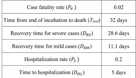
On the other hand, one needs additional information on the infection fatality ratio (i.e., the proportion of infected individuals who die eventually) and on the distribution of

Figure 2: The trend of COVID-19 confirmed cases and recovered cases in Ukraine based on COVID-19 and population datasets.. We assume that morbidity by novel coronavirus infection

We analyze an epidemic model on a network consisting of susceptible- infected-recovered equations at the nodes coupled by diffusion using a graph Laplacian.. We introduce an

The fraction of reported cases, from date τ 3 to date τ f , the fraction of reported cases f was assumed increase linearly to reach the value 200% of its initial one and the fraction

COMOKIT combines models of person-to-person and environmental transmission, a model of individual epidemiological status evolution, an agenda-based 1-h time step model of

[5] studied a SIRS model epidemic with nonlinear incidence rate and provided analytic results regarding the invariant density of the solution.. In addition, Rudnicki [33] studied