Science Arts & Métiers (SAM)
is an open access repository that collects the work of Arts et Métiers Institute of
Technology researchers and makes it freely available over the web where possible.
This is an author-deposited version published in: https://sam.ensam.eu Handle ID: .http://hdl.handle.net/10985/8577
To cite this version :
Abdelkader ZAARAOUI, Florent RAVELET, Florent MARGNAT, Sofiane KHELLADI - High Accuracy Volume Flow Rate Measurement Using Vortex Counting - Flow Measurement and Instrumentation - Vol. 33, p.138-144 - 2013
Any correspondence concerning this service should be sent to the repository Administrator : [email protected]
High Accuracy Volume Flow Rate Measurement Using Vortex Counting
A. Zaaraouia, F. Raveletb,∗, F. Margnatb, S. Khelladib
aLaboratoire Fluides Industriels Mesures et Applications, Universit´e de Khemis Meliana, Alg´erie. bArts et Metiers ParisTech, DynFluid lab., 151 boulevard de l’Hˆopital, 75013 Paris, France.
Abstract
A prototype device for measuring the volumetric flow-rate by counting vortices has been designed and realized. It consists of a square-section pipe in which a two-dimensional bluff body and a strain gauge force sensor are placed. These two elements are separated from each other, unlike the majority of vortex apparatus currently available. The principle is based on the generation of a separated wake behind the bluff body. The volumetric flow-rate measurement is done by counting vortices using a flat plate placed in the wake and attached to the beam sensor. By optimizing the geometrical arrangement, the search for a significant signal has shown that it was possible to get a quasi-periodic signal, within a good range of flow rates so that its performances are well deduced. The repeatability of the value of the volume of fluid passed for every vortex shed is tested for a given flow and then the accuracy of the measuring device is determined. This quantity is the constant of the device and is called the digital volume (Vp). It has the dimension of a volume and varies
with the confinement of the flow and with the Reynolds number. Therefore, a dimensionless quantity is introduced, the reduced digital volume (Vr) that takes into account the average speed in the contracted section downstream of the
bluff body. The reduced digital volume is found to be independent of the confinement in a significant range of Reynolds numbers, which gives the device a good accuracy.
Keywords: Wake; Bluff body; Accuracy; Strain gauges sensor; Vortex shedding; Digital volume.
1. Introduction
Measurements of volumetric flow rates are common practices in fluid flow under pressure. The devices that are available and the corresponding techniques are of var-ious types but generally guarantee a precision that rarely exceeds 1%. However, the current needs of certain indus-tries (petroleum, chemical etc...) go beyond that figure. To meet this demand, a solution is provided by methods of measurement based on counting the vortices generated in the wake of a bluff body in a two-dimensional flow.
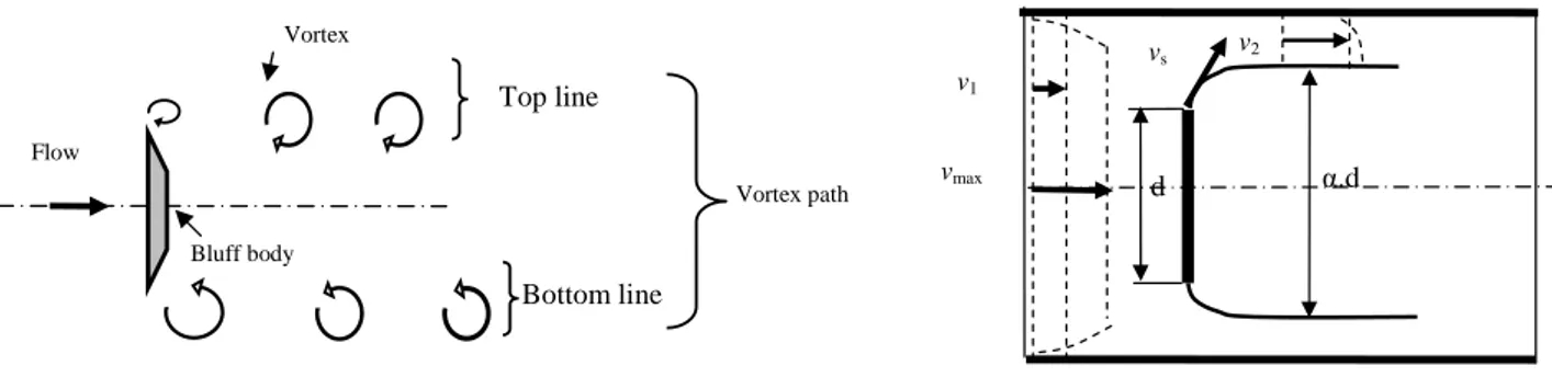
In a free medium, for a perfect fluid, the wake down-stream of a bluff body is characterized by the presence of two parallel vortex sheets where the vorticity is concen-trated [1, 2]. For a real fluid, the configuration depends on the Reynolds number, usually based on the free-stream velocity v1and a typical length of the cross-section of the
bluff body d (see figure 1 left). At very low Reynolds number (of the order of the unity) the flow is steady and presents all the symmetries of the problem. As the Reynolds number increases, the vortex sheets first give nice sta-ble and periodic roller shaped vortices to form the “von K´arm´an vortex street” (see figure 1). For Reynolds num-bers of the order of 102, there is a unique frequency f that
is usually given in a dimensionless form with a Strouhal
∗corresponding author
Email address: [email protected] (F. Ravelet)
number St = f ·d
v1. In this intermediate Reynolds num-bers range, the Strouhal number varies with the Reynolds number monotonically. For large Reynolds number (in the range 103− 105) a wake with a certain periodicity is still
observed in spite of the instabilities: the vortices now do not detach on a regular basis, but the frequency spectrum of the wake presents a peak at a well-defined frequency f . The Strouhal number becomes moreover independent of the Reynolds number [1, 3–5].
In the case of a two-dimensional flow that is confined between two parallel plates separated by a distance D (see figure 1, right), the relative confinement of the flow (d
D) is
an additional parameter that may influence the behaviour of the flow. The downstream flow qualitatively exhibits the same phenomena as that observed in the case of a free medium: the wake is still well formed, limited by two streamlines with a constant average pressure and there ex-ists a main frequency. Studies of several researchers show that parameters such as the confinement, the turbulence, the end effects, the geometric shape and the vibration of the bluff body affect quantitatively the overall value of the Strouhal number [6–11]. One question is to identify the choice of typical length scale and velocity scale that would give the simplest expression of a Strouhal number as a function of the Reynolds number and the confinement.
Based on this principle, several techniques have been used for the construction of flowmeters with vortex effect that are different by the way of generating or capturing the
hal-00707329, version 4 - 17 Jun 2013
Author manuscript, published in "Flow Measurement and Instrumentation (2013) 1" DOI : 10.1016/j.flowmeasinst.2013.06.002
3
In a confined medium (Figure 2), the flow is two dimensional and velocity fields are contained between two parallel planes. The bluff body was placed at the center of the pipe and the study of the downstream flow qualitatively gives the same phenomena that occur in the case of the free medium flow. To study the influence of geometric parameters, such as
confinement of the fluid vein
(
)
D
d
, we usually use the Strouhal number (St1) formed with upstream and discharge velocity d
and
v
. Studies of several researchers show that parameters such as the confinement, the turbulence, the end effects, the geometric shape and the vibration of the bluff body affect the overall value of the Strouhal number (St1) [1, 2, 4, 6, 14 and 19].In the flow inside a pipe, introducing the volume flow rate
q
v , we obtain the following expression:f
q
v = tS
A
d.
= Cte , whereA is the section of the pipe. This relationship shows that the flow rate is proportional to the frequency of the vortex shedding. The proportionality coefficient characterizes the transition of the vortex in question and whose performance depends on the geometric arrangement of the elements that constitute the device.
Vortex path Bottom line Bluff body Top line Vortex Flow
Figure 1 : Vortex path
4
Based on this principle, several techniques have been used for the construction of flowmeters with vortex effect that are different by the way of generating or capturing the eddies and among which we quote:
Z. Sun et al [3 and 17] measure the pressure difference hence the frequency of vortex shedding. The sensing is performed at the bluff body with sharp edges. J. Peng et al [10 and 18] use configurations with two bluff bodies for the generation of vortices. The frequency is determined by measuring fluctuations using two piezoelectric pressure sensors placed at the second hurdle. V. Hans et al [5] present a technique that uses a bluff body with a triangular base and the detection is performed using two ultrasonic probes. S.C Bera et al [11] use a technique called inductive pick-up that uses a flexible magnetic strip made of Stainless Steel and placed just downstream of the bluff body to determine of frequency. S. Takashima et al [12] have used a bluff body of square section and a double FBG sensor (a technique that uses the interferometric detection to count electromagnetic interference). JJ Miau et al [13] presented in their paper a technique where the bluff body and the sensor are the same piece. A T-shaped bluff body to which is attached a piezoelectric pressure sensor is used, to determine the frequency. We note that in almost all the work presented, the conduct of circular section hinders the formation of vortex roll since the latter is crushed on both ends. Moreover the detection is done at a point only and early in the vortex formation. The results of there studies give the frequency spectrum of vortex shedding, the Strouhal number variation with Reynolds number and the influence of geometry on flow measurement.
In the case of the volume measurement, the constant of the device is called digital volume (Vp) which is the inverse of the
Strouhal number: it is the volume between the passage of two successive vortice rolls of the same line of the vortex path. A technique for generating and counting vortices will be used in this work and whose originality is to use a section of pipe with quadrangular cross-section and to separate the generation function from that of detection. The aim is high accuracy measurement of volume. Generation is provided by bluff body of a trapezoidal section with two parallel sharp edges, behind which vortices develop. The detection is of a surface type and is perfomed at some distance downstream of the obstacle. It is
Figure 2: Two dimensional flow in confined
α.d vmax vs d v2 v1
Figure 1: Left: illustration of the vortex path past a bluff body for a flow in infinite medium. Right: sketch of the two-dimensional confined flow between two plates separated by D, with a bluff body of cross-section d.
eddies. For instance, Sun et al. [12, 13] use a bluff body with sharp edges on which the pressure difference, hence the frequency of vortex shedding, is measured. Peng et al. [14, 15] use configurations with two bluff bodies for the generation of vortices. The frequency is determined by measuring fluctuations using two piezoelectric pressure sensors placed at the second hurdle. Hans et al. [16] present a technique that uses a bluff body with a triangu-lar base and two ultrasonic probes for the detection. Bera et al. [17] use a technique called “inductive pick-up” that uses a flexible magnetic strip made of Stainless Steel and placed just downstream of the bluff body to determine the frequency. Takashima et al. [18] have used a bluff body of square section and a double Fiber Bragg grating (FBG) sensor (a technique that uses the interferometric detection to count electromagnetic interference). Miau et al. [19] present in their paper a technique where the bluff body and the sensor are the same piece. A T-shaped bluff body to which is attached a piezoelectric pressure sensor is used, to determine the frequency. We note that in almost all the work presented, the pipe of circular section hinders the for-mation of vortex roll since the latter is crushed on both ends. Moreover the detection is done at a single point that is quite close to the vortex formation. The results of these studies give the frequency spectrum of vortex shedding, the Strouhal number variation with Reynolds number and the influence of geometry on flow measurement.
The measurement system that is presented thereafter is based on this principle. The originality is to use pipe with square-section in order to get closer to a two-dimensional flow and to separate the generation function from that of detection. Generation is provided by bluff body of trape-zoidal section with two parallel sharp edges, behind which vortices develop. The detection is of surface type and is performed at some distance downstream of the obstacle. It is done via a flat plate, parallel to the flow and secured to a beam bending over which are fixed strain gauges. The successive passages of the vortices near the plate stress the beam. The strain gauge transforms the elastic defor-mation into an electrical signal which, after amplification, accurately reflects the nature of the mechanical vibrations. In principle the number of vortices which are issued and
counted during a given time should be directly related to the volumetric flow-rate.
The experimental setup is described in § 2. To evaluate the precision of the apparatus, and to study the effects of the confinement and of the distance between the actuator and the sensor, a specific test loop has been built. The apparatus is first described in § 2.1, and the test loop is described in § 2.2. The accuracy of the measurements is discussed in § 2.3. The results are presented and discussed in § 3: the search for an optimal position of the bluff body in the pipe and the analysis of the sensitivity of the vortex street to the various geometric parameters is presented in § 3.1 and the effects of the confinement on the calibration of the apparatus are presented in § 3.2. Final remarks and perspectives are then given in § 4.
2. Experimental setup and measurement technique
2.1. Geometry of the flowmeter
The technique used in the apparatus shown in figure 2 is based on the generation and detection of vortices with two distinct devices: one for each function. The measure-ments are performed in a measurement tunnel of square section D × D. The direction of the flow is denoted x. A bluff body of cross-section d × D in the {y ; z} plane is secured in the middle of the measurement tunnel (see figure 2, left). This bluff body is of trapezoidal section in the {x ; y} plane and thus presents two sharp edges to the flow. The sensor consists of a flat plate parallel to the flow. It is of length Lp in the x direction, and placed at
a distance l from the bluff body. It is secured to a bend-ing beam over which are fixed strain gauges (see figure 2, right).
2.2. Description of the dedicated test bench
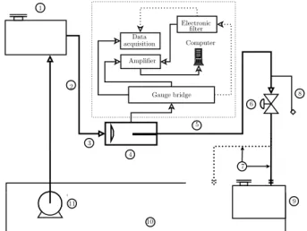
The hydraulic system is shown in figure 3 and is de-signed to cover a range of flow rates from 0 to 50 m3/h.
We show successively:
• a pressurized supply tank (1) with open surface lo-cated at a height of 11 m, and of capacity 20 m3;
2
6
3. Experimental setup and procedure.
The hydraulic system is shown in Figure 6 and is designed to cover a range of flow rates from 0 to 50 m3
/ h. We find successively:
• a pressurized supply tank (1) with open surface located at a height of 11 meters, and of capacity 20 m3. • A distribution pipe brass (2) 10 meters in length and 200 mm in inner diameter, terminated by a supply valve. • Another line consisting of PVC pipes (3) 80 mm in diameter.
• A testing tunnel (4) which houses the generator and the vortex sensor is connected to a measuring system comprising various devices for measurement, display and acquisition.
• Finally, another pipe of 80 mm in diameter made of PVC (5) ending in gooseneck and provided with a valve (6). In parallel there is a flexible hose (7) with a quick release nozzle (8) (similar to gasoline pumps in service stations).
Figure 4 : Vortex sensor Strain gauges Flat plate Bending beam Lp ep A A A-A Trapezoidal section B B D d
Figure 5 : Bluff body
B-B D Lp Sensor Bluff body D d Flow l
Figure 3: Geometric arrangement for the proposed technique
6
3. Experimental setup and procedure.The hydraulic system is shown in Figure 6 and is designed to cover a range of flow rates from 0 to 50 m3 / h. We find successively:
• a pressurized supply tank (1) with open surface located at a height of 11 meters, and of capacity 20 m3. • A distribution pipe brass (2) 10 meters in length and 200 mm in inner diameter, terminated by a supply valve. • Another line consisting of PVC pipes (3) 80 mm in diameter.
• A testing tunnel (4) which houses the generator and the vortex sensor is connected to a measuring system comprising various devices for measurement, display and acquisition.
• Finally, another pipe of 80 mm in diameter made of PVC (5) ending in gooseneck and provided with a valve (6). In parallel there is a flexible hose (7) with a quick release nozzle (8) (similar to gasoline pumps in service stations).
Figure 4 : Vortex sensor Strain gauges Flat plate Bending beam Lp ep A A A-A Trapezoidal section B B D d
Figure 5 : Bluff body B-B D Lp Sensor Bluff body D d Flow
l
Figure 3: Geometric arrangement for the proposed technique
Figure 2: Geometric arrangement for the proposed technique. Details of the bluff body and of the vortex sensor.
• a distribution brass pipe (2) of length 10 m and inner diameter 200 mm, terminated by a supply valve; • another line consisting of PVC pipes (3) of diameter
80 mm;
• a testing tunnel (4) which houses the generator and the vortex sensor connected to a measuring system consisting of various devices for measurement, dis-play and acquisition;
• another pipe of diameter 80 mm made of PVC (5) ending in gooseneck and provided with a valve (6); • in parallel a flexible hose (7) with a quick release
nozzle (8) (similar to gasoline pumps in service sta-tions);
• a receiving gauged tank with a capacity of 1 m3 (9),
in parallel with a recovery pit (10) located below the floor;
• a flexible conduit (7) attached to the goose-neck that can guide the jet, either toward the pit or to the gauge volume for measurements;
• a centrifugal pump (11), to pump the fluid between the tank and supply tank.
The measuring system includes the main following com-ponents:
• a strain gauge Vishay-micromeasurement which is a Wheatstone bridge specially designed for use with strain gauges operating in bending;
• a computer-amplifier based on the principle of syn-chronization of a square wave signal with the signal delivered by the strain gauge;
• a passband electronic filter to eliminate the back-ground noise and possible irregularities that can some-times plague the signal;
• a data acquisition system.
The tests are performed using a protocol that consists of filling the gauged tank by operating at constant average flow, for a given value of the confinement d
D (ratio of
char-acteristic dimensions of the bluff body and testing tunnel). A wide range of flow-rates are tested for each configura-tion. Several geometrical arrangement of the generator and sensor, i.e. several combinations of l and Lp, have
been tested. The quantities obtained by the measuring devices are: volume V (close to 1000 litres), the number of vortices N (near 4000) and the corresponding time t to fill the gauge.
The calculated quantities are:
• the digital volume, i.e. the volume of fluid passed for every vortex shed Vp=NV;
1 2 3 4 5 6 7 8 9 10 11 Data acquisition Electronic filter Amplifier Computer Gauge bridge 1
Figure 3: Sketch of the test loop.
• the mean frequency of vortex shedding f = N
t;
• the average flow rate qv=Vt;
• a Reynolds number based on the characteristic di-mension of the testing tunnel (D) and on the dis-charge velocity:
ReD=
qvD
Atν
with Atthe tunnel cross-section and ν the kinematic
viscosity of water;
• a Reynolds number based on the characteristic di-mension of the obstacle generator (d) and on the same velocity scale:
Red=
qvd
Atν
• a Strouhal number based on the bluff body charac-teristic length d, and on the same velocity scale:
St=
f · d qv/At
• a dimensionless (reduced) digital volume: Vr=
Vp
d · D2· f (d/D)
with f (d/D) a function that will be introduced there-after in order to give a universal reduced digital vol-ume that will only depend on the Reynolds number. 2.3. Accuracy of the measurements
The objective of this flow-meter is to give a measure of the flow-rate that is as accurate as possible. The typ-ical constancy of the calibration factor for the considered
class of flow-meters is of the order of ±0.7% — ±1% over a dynamic range of 3 — 6 [1, 3, 10, 13, 19]. In order to find the calibration with a relative precision of let’s say ±0.1% of the measured value, it is first necessary to mea-sure the volume, the number of vortices and the time with a resolution better than ±0.1%.
It it necessary to distinguish between three types of volumes used in the same operation:
1. The volume disposed from the upstream reservoir V1and discharged at the outlet conduit between the
first and the last valves.
2. The displayed volume V2 of the volume gauge of
about 1000 litres. It is known with an uncertainty of reading of δV2= 0.25 litre. This volume is equal to
that received by the dry gauge, otherwise it differs by a certain amount ∆V2= 1 litre due to the water
film wetting the inner wall of the gauge; we have in fact: V1 = V2− ∆V2± δV2. If we suppose that the
wettability remains the same, ∆V2 can be regarded
as a constant.
3. The counted volume V3 that defines the number of
vortices indicated by the electronic counter, we have: V3= N ·Vp. It is not equal to V1for two reasons. The
first is that since N is an integer, a mistake of one unit at the beginning and at the end of counting can be made, which results in an uncertainty of about 2. The second reason is of physical origin and depends on the method used to fill the gauge. We can write V1= V3± (2 + δN )Vp.
It comes as an apparent digital volume: V2 N = Vp(1 ± ( 2 + δN N )) + ∆V2 N ± δV2 N
Suppose that δN = 2 and that N ' 4000. For a digital volume to be measured Vp of the order of Vp' 0.25 litre,
the maximum relative uncertainty of the digital volume measurement is 2.25 × 10⁻³, but working under the same
conditions of wetting of the gauge, the value is reduced to 1.25 × 10⁻³.
The calculation of the characteristic quantities and the corresponding uncertainties give a maximum relative error of the order of 0.4%, so that the relative variations of quan-tities around their mean value are of the order of ±0.2%. These small variations do not affect the calculation of the average digital volume.
3. Results
3.1. Optimal geometric layout and representative frequency signals
The desired relative accuracy is of the order of one thousandth of the measured value. The greatest care and every precaution then have to be taken in order to obtain significant repetitive signals. Hundreds of observations of digitized signals have been made and those which seemed 4
Figure 4: Representative Signals of the shedding vortices frequency.
most significant have been selected and are shown in fig-ure 4.
The geometric arrangement directly affects the qual-ity of the electric signal collected at the output of the strain gauge. The surface detection type that is used in the present apparatus, in contrast to the volume and point detection types, may result in an easily exploitable signal, providing a good choice of the geometric arrange-ment. The geometric parameters that can influence the correct operation of the measuring device and thus ensure the accuracy are:
• the width of the sensor plate (Lp);
• the distance between the bluff body and the sensor (l);
• the material and thickness of the plate used to detect vortices (ep);
• the orientation of the sensor plate with respect to the flow direction;
• the misalignment of the vortices generator relative to the axis of the pipe.
Without entering into the details of the analysis, our goal is to get significant and repetitive signals. Therefore the shape of the signal has been studied for different geo-metric configurations. An unfiltered signal may result in double counting of vortices (signal 6). Other signals that are not exploitable (signals 1, 2, 3, 8, 9 and 10) are ex-amples of the deleterious effects of the material used for the sensor, the thickness of the plate, a bad balance of the natural bluff body, a very large or very small width of the plate, or a bad plate bluff body.
By optimizing the geometric layout, the search for a significant signal showed that it was entirely possible to
have a quasiperiodic signal for all flow rates (signals 4, 5 and 7). For a bluff body of a given dimension, this optimization is characterized by the following parameters:
• a thickness of ep= 0.7 mm for the plate sensor;
• a width Lp of 1.5d to 2d for the plate sensor;
• a bluff body-plate sensor distance l of 3.5d to 4.5d. 3.2. Effects of the geometrical confinement on the digital
volume
In a first step, for a given configuration, tests were performed to see how accurately the digital volume value repeats itself. The results show that if the measurements are repeated with the same conditions, a constant value which reproducibility is better than 10−3and a very small
variation of the digital volume with the flow rate are found. The values of Vp for d = 15 mm, i.e. for a containment
of d
D = 0.25 and for two flow-rates are reported in Tab. 1.
More values are displayed in figure 5.
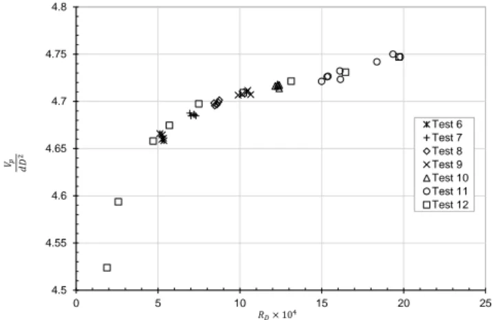
4.5 4.55 4.6 4.65 4.7 4.75 4.8 0 5 10 15 20 25 Test 6 Test 7 Test 8 Test 9 Test 10 Test 11 Test 12 𝑅𝐷× 104
Figure 5: Reproducibility of digital volume changes with the
Reynolds number, bluff body characteristic dimension d = 15mm (confinement Dd = 0.25).
The figure 5 shows that for a given containment, the digital volume indeed depends on the Reynolds number ReD, hence on the flow rate of the pipeline. The digital
volume increases with the flow rate: the variation is much stronger at low values of Reynolds number, and one can notice some stabilization for the highest values. Further-more, the excellent reproducibility of the curve with an accuracy of ±0.1% is once more verified.
The next step is to find the most significant dimension-less representation of the digital volume that would take into account the effects of the confinement.
The digital volume is: Vp=
V N =
qv
f
If we introduce the Strouhal number St, we get:
Vp=
D2d St
Flow rate qv (litre/s) Digital Volume Vp(litres)
Test 1 Test 2 Test 3 Test 4 Test 5 1.56 0.24805 0.24821 0.24814 0.24802 0.24827 4.53 0.25366 0.25385 0.25368 0.25361 0.25381
Table 1: Digital volume Vpfor Dd = 0.25.
By dimensional analysis, the Strouhal number is a function of the confinement and of the Reynolds number:
St= g(
d D, Red) It will be shown in the following that g(d
D, Red) can be
written as the product of two functions of only d
D and Red, i.e.: g(d D, Red) = f ( d D) · h(Red) 4 4.2 4.4 4.6 4.8 5 5.2 5.4 5.6 5.8 0 5 10 15 20 25 d/D = 0.166 d/D = 0.238 d/D = 0.272 d/D = 0.288 𝑅𝐷× 104
Figure 6: Variation of the dimensionless digital volume with the Reynolds number of the pipe for different confinements.
The variations of Vp
dD2 —that is thus the inverse of the previously defined Strouhal number St— with the
con-finement d
D and the Reynolds number Red are therefore
separately studied in the next paragraphs. The results are plotted in figure 6, as functions of the Reynolds number for various confinements. The curves look overall the same: there is a very slight increase of the dimensionless digital volume with the Reynolds number. For a fixed confine-ment, the digital volume varies by roughly 2% whilst the Reynolds number varies by one order of magnitude. This variation moreover may be well represented by a unique h(Red) function with a prefactor depending only on the
confinement. For a constant Reynolds number, the digital volume decreases with an increase of the confinement. The dependence with the confinement is more significant: for the two extreme cases that are presented in figure 6, i.e. d= 0.166 and 0.288 the variation of the digital volume is roughly of the order of 60%.
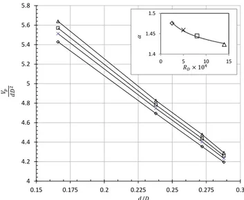
4 4.2 4.4 4.6 4.8 5 5.2 5.4 5.6 5.8 0.15 0.175 0.2 0.225 0.25 0.275 0.3 𝑑/𝐷 1.4 1.45 1.5 0 5 10 15 𝑅𝐷× 104
Figure 7: Variation of the dimensionless digital volume with con-finements for several Reynolds numbers (ReD). Inset: parameter α vs. ReD, where the parameter α is obtained by a fit of the form
Vp
dD2 = Vr(ReD) · (1 − αDd).
The dimensionless digital volume Vp
dD2 as a function of the confinement d
D at different constant Reynolds numbers
is plotted in figure 7. The results show that the function f(d
D) may be well represented by a function of the form
f(x) = a · x + b. A simple interpretation can be found if this dependence is written in the equivalent form:
f(x) = Vr· (1 − αx)
The results show that α only has a very slight dependence with the Reynolds number (see inset in figure 7).
The value of α is interpreted as the width of the wake behind the bluff body (see Fig. 1, right). Let us define a second Strouhal number with the velocity of the wake v2= qv(D − αD))−1:
St2=
f d v2
Then the “reduced digital volume” is the inverse of this second Strouhal number, that seems to be only a function of the Reynolds number:
Vr=
Vp
dD2(1 − αd
D)
Owing to the negligible dependence of α with ReD, a
constant value of α = 1.455 is assumed to compute the 6
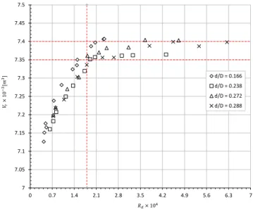
7 7.05 7.1 7.15 7.2 7.25 7.3 7.35 7.4 7.45 7.5 0 0.7 1.4 2.1 2.8 3.5 4.2 4.9 5.6 6.3 7 d/D = 0.166 d/D = 0.238 d/D = 0.272 d/D = 0.288 𝑅𝑑× 104
Figure 8: Universal curve (variation of the reduced digital volume).
reduced digital volume. The variation of Vr with Red is
plotted in figure 8. All the results are grouped around a universal curve with an accuracy of about 0.3%: this dimensionless representation shows that the reduced digi-tal volume is independent of the confinement of the fluid stream. The reduced digital volume Vr varies slightly
at low Reynolds numbers. A plateau is obtained past a threshold in the Reynolds number equal to 1.8 × 10⁴: a
constant value of Vr = 7.373 is obtained with an
accu-racy of ±3 × 10⁻³, a value slightly lower than the target,
in the range 1.8 × 10⁴ ≤ Re
d ≤ 6.3 × 10⁴, a dynamic
range of about 4.5 which is comparable to the state of the art [1, 3, 10, 13, 19]. The latter might be improved by using a testing tunnel of rectangular section.
4. Conclusions
The designed and produced apparatus is suitable for measurements of flow rates averaged for a sufficiently long time. To design and implement an accurate volumetric flow rate measurement unit through the vortex street or the wake generated by a bluff body, an optimal geometrical arrangement of the bluff body, the sensor and the testing tunnel has been suggested that should lead to the best pos-sible signal quality and thus to minimize the errors. The variation of the digital volume with the confinement and with the Reynolds number, led us to define a reduced dig-ital volume Vr. It is a dimensionless quantity equal to the
inverse of the Strouhal number defined with the average velocity in the contracted section downstream of the bluff body. The reduced digital volume has a constant value equal to 7.373. It is a constant of the proposed volume counter. It is represented by a universal curve indepen-dent of the geometric parameters. The relative accuracy of our device is about ±0.3% in a range of flow rates from 3.0 l/s to 13.3 l/s, which is noteworthy result.
References
[1] T. Ghaoud and D.W. Clarke. Modelling and tracking a vor-tex flow-meter signal. Flow Measurement and instrumentation, 13:103–117, 2002.
[2] C.H.K. Williamson and R. Govardhan. A brief review of recent
results in vortex-induced vibrations series. Journal of Wind
Engineering and Aerodynamics, 96:713–735, 2008.
[3] J.J. Miau, C.W. Wu, C.C. Hu, and J.H. Chou. A study on signal quality of a vortex flow meter downstream of two elbows out-of-plane. Flow Measurement and instrumentation, 13:75– 85, 2002.
[4] J.P. Bentley and J. Mudd. Vortex shedding mechanisms in sin-gle and dual bluff bodies. Flow Measurement and instrumenta-tion, 14:23–31, 2003.
[5] G. L. Pankanin, A. Kulinczak, and J. Berlinski. Investigation of karman vortex street using flow visualization and image pro-cessing. Sensors and Actuators, A 138:366–375, 2007. [6] S. Goujon-Durand. Technical note, linearity of the vortex meter
as function of fluid viscosity. Flow Measurement and instrumen-tation, 6(3):235–238, 1995.
[7] J.P. Bentley, R.A. Benson, and A.J. Shanks. The development of dual bluff body vortex flow meters. Flow Measurement and instrumentation, 7(2):85–90, 1996.
[8] C.H.K. Williamson. A series in √1
re to represent the
strouhal-reynolds number relationship of the cylinder wake. Journal of Fluids and Structures, 12:1073–1085, 1998.
[9] J.J. Miau, C.C. Hu, and J.H. Chou. Reponse of a vortex flow meter to impulsive vibrations. Flow Measurement and instru-mentation, 11:41–49, 2000.
[10] H. Zhang, Y. Huang, and Z. Sun. A study of mass flow rate measurement based on the vortex shedding principle. Flow Mea-surement and instrumentation, 17:29–38, 2006.
[11] A. Venugopal, A. Agrawal, and S.V. Prabhu. Influence of block-age and upstream disturbances of the performance of a
vor-tex flowmeter with a trapezoidal bluff body. Measurement,
43(4):603–616, 2010.
[12] Z. Sun, H. Zhang, and J. Zhou. Investigation of the pressure probe properties as the sensor in the vortex flowmeter. Sensors and Actuators, A 136:646–655, 2007.
[13] J. Zhou Z. Sun, H. Zhang. Evaluation of uncertainty in a vortex flowmeter measurement. Measurement, 41:349–356, 2008. [14] J. Peng, X. Fu, and Y. Chen. Flow measurement by new type
vortex flowmeter of dual triangulate bluff body. Sensors and Actuators, A 115:53–59, 2004.
[15] J. Peng, X. Fu, and Y. Chen. Experimental investigations of strouhal number for flows past dual triangulate bluff bodies. Flow Measurement and instrumentation, 19:350–357, 2008. [16] V. Hans and G. Poppen. Vortex shedding flow meters and
ultra-sound detect ion: signal processing and influence of bluff body
geometry. Flow Measurement and instrumentation, 9:79–82,
1998.
[17] S.C Bera, J.K. Ray, and S. Chattopadhyay. A modified induc-tive pick-up type technique of measurement in a vortex flow meter. Measurement, 35:19–24, 2004.
[18] S. Takashima, H. Asanuma, and H. Niitsuma. A water flowme-ter using dual fiber bragg grattting sensors and cross-correlation technique. Sensors and Actuators, A 116:66–74, 2004. [19] J.J. Miau, C.F. Yeh, C.C. Hu, and J.H. Chou. On measurement
uncertainty of a vortex flow meter. Flow Measurement and
instrumentation, 16:397–404, 2005.
Nomenclature
Roman characters
At [m2] tunnel cross-section
d [m] charcteristic dimension of the bluff body
D [m] characteristic dimension of the test section
ep [m] thickness of the plate sensor
f [Hz] mean vortex shedding frequency
l [m] distance between the vortex generator and the plate sensor
Lp [m] length of the plate sensor
N [−] number of counted vortices
qv [m3· s−1] volumetric flow rate
Red [−] Reynolds number based on d
ReD [−] Reynolds number based on D
St [−] Strouhal number based on f , d and discharge velocity
St2 [−] Strouhal number based on f , d and v2
t [s] time to fill the gauge
v1 [m3· s−1] free-stream velocity
v2 [m3· s−1] velocity of the wake
V [m3] total volume passed through the test section
V1 [m3] volume discharged
V2 [m3] displayed volume of the volume gauge
V3 [m3] counted volume
Vp [m3] digital volume
Vr [−] reduced digital volume
Greek characters
α [−] relative width of the wake
δV2 [m3] reading uncertainty of V2
δN [-] uncertainty of vortex counting
∆V2 [m3] volume loss due to wettability
ν [m2· s−1] kinematic viscosity
8