Deep-learning for high dimensional sequential observations : application to continuous gesture recognition

(1)

HAL Id: tel-02012106

https://tel.archives-ouvertes.fr/tel-02012106

Submitted on 8 Feb 2019

HAL is a multi-disciplinary open access

archive for the deposit and dissemination of sci-entific research documents, whether they are pub-lished or not. The documents may come from teaching and research institutions in France or abroad, or from public or private research centers.

L’archive ouverte pluridisciplinaire HAL, est destinée au dépôt et à la diffusion de documents scientifiques de niveau recherche, publiés ou non, émanant des établissements d’enseignement et de recherche français ou étrangers, des laboratoires publics ou privés.

Deep-learning for high dimensional sequential

observations : application to continuous gesture

recognition

Nicolas Granger

To cite this version:

Nicolas Granger. Deep-learning for high dimensional sequential observations : application to continu-ous gesture recognition. Human-Computer Interaction [cs.HC]. Université Paris-Saclay, 2019. English. �NNT : 2019SACLL002�. �tel-02012106�

(2)

(3)

Abstract

The original impulse for this thesis came as a motivation to improve the intuitiveness of human–computer interfaces. In particular, machines should try to replicate human’s ability to process streams

of information continuously in real-time. Indeed, reading, listening to speeches or observing a live scene are all natural activities we perform spontaneously and use extensively to interact or communicate. However, the sub-domain of Machine Learning dedicated to recognition on time series remains barred by numerous challenges: modelling patterns simultaneously over time and within individual observations, dealing with high dimensional inputs from streams of observations, conforming to real-time specifications, etc. Nevertheless, this research field has progressed steadily over the last decades, with a recent renewal fuelled by advances on Neural Network models.

To support our studies on this subject, gesture recognition was selected as the exemplar appli-cation. This type of input presents several qualities in our eyes: firstly, gestures intermix static body poses and movements in a complex manner to convey information; secondly, gesture data is encoded under widely different modalities with low and high dimensional representations; finally, the lack of expertise in this field — compared to handwriting or speech recognition — emphasizes better the importance of automatically learning useful factors of variation, which conditions cross-domain re-usability.

The first part of our work examines two state-of-the-art temporal models used in the context of continuous sequence recognition, namely Hybrid Neural Network–Hidden Markov Models (NN-HMM) and Bidirectional Recurrent Neural Networks (BDRNN) with gated units. Instead of trying to improve their performances for a given task, this thesis puts more emphasis on analyzing shortcomings, advantages, similarities or influential properties. To do so, we reim-plement the two within a shared test-bed for continuous sequence recognition which is more amenable to a fair comparative work. We propose adjustments to Neural Network training loss functions and the Hybrid NN-HMM expressions to accommodate for highly imbalanced data classes. Although most of recent contributions tend to prefer the Recurrent Neural Networks on the basis of superior performances, we demonstrate that both models can in fact perform competitively. However, our experiments also exhibit that Hybrid NN-HMM rely more on their input transformation modules, in particular on the existence of a short-term temporal pattern detector which we implement via Temporal Convolutions. Finally, we demonstrate inter-compatibility between the representation learning stages of both solutions, indicating a convergence of representations to encode factors of variations in the inputs.

Between humans, interactions and communications necessitate more that comprehension alone, as we also learn and adapt quickly to novelties in our environment: new words, voices,

(4)

symbols, etc. The pendant of this capability in Machine Learning is formalized under the one-shot learning setting, which has been the subject of relatively few research works so far, in particular for sequential inputs. To tackle this problem, we propose a model built around a Bidirectional Recurrent Neural Network. Its effectiveness is demonstrated by testing the dis-criminative performances on isolated gestures recordings from a sign language lexicon. We propose several improvements over this baseline by drawing inspiration from related works and evaluate their performances, exhibiting different advantages and disadvantages for each.

(5)

Résumé

Cette thèse a pour but de contribuer à améliorer les interfaces Homme-machine. En particulier, nos appareils devraient répliquer notre capacité à traiter continûment des flux d’informations. En effet, nous lisons, écoutons et observons des scènes spontanément pour interagir ou com-muniquer. Cependant, le domaine de l’apprentissage statistique dédié à la reconnaissance de séries temporelles pose certains défis : la détection de phénomènes définis simultanément dans le temps ou dans l’instant, le traitement de flux de données de grandes dimensions, l’inférence en temps réel, etc. Néanmoins, la recherche dans ce domaine a progressé continuellement au cours des dernières décennies, avec un nouveau souffle apporté par les récents progrès avec les réseaux de neurones.

Pour appuyer notre étude de ce sujet, nous avons sélectionné la reconnaissance de gestes comme exemple applicatif. Ce type de données présente de multiples avantages à nos yeux : premièrement, la signification des gestes repose sur un mélange complexe de poses corporelles et de mouvements, deuxièmement, les gestes sont encodés sous des formes très variées avec des représentations en faible ou grande dimension; enfin, la faible expertise présente dans ce domaine —comparé à l’écriture ou la parole— permet de mieux mettre en valeur l’importance de l’apprentissage automatique de représentations, qui conditionne la facilité à réutiliser un modèle sur des domaines différents.

La première partie de notre travail examine deux modèles temporels de l’état de l’art pour la re-connaissance continue sur des séquences, plus précisément l’hybride réseau de neurones–modèle de Markov caché (NN-HMM) et les réseaux de neurones récurrents bidirectionnels (BD-RNN) avec des unités commandées par des portes. Plutôt que de consacrer notre étude à l’optimisation des performances, cette thèse se focalise sur l’analyse des propriétés majeures caractérisant ces deux modèles. Pour ce faire, nous avons implémenté un environnement de test partagé qui est plus favorable à une étude comparative équitable. Nous proposons des ajustements sur les fonc-tions de coût utilisées pour entraîner les réseaux de neurones et sur les expressions du modèle hybride afin de gérer un large déséquilibre des classes de notre base d’apprentissage. Bien que les publications récentes semblent privilégier l’architecture BD-RNN, nous démontrons qu’il est possible d’obtenir des performances comparables avec l’autre approche. Néanmoins, nos expér-iences montrent aussi que le succès de l’hybride NN-HMM est conditionné sur la modélisation des entrées dans les premières couches du modèle. Celles-ci doivent en particulier modéliser les phénomènes temporels à court terme que nous détectons à l’aide de convolutions temporelles. Nous montrons aussi que ces représentations sont largement inter-compatibles entre les deux modèles, ce qui démontre une convergence dans la manière d’encoder les facteurs de variations des entrées.

(6)

La compréhension ne représente qu’un seul aspect des échanges et interactions entre hu-mains. Nous utilisons aussi largement notre faculté à apprendre et à s’adapter rapidement à des nouveautés de notre environnement : de nouveaux mots ou symboles, de nouvelles voix, etc. L’équivalent de cette faculté en apprentissage statistique est formalisé par le paradigme de l’apprentissage dit « en un coup », qui a reçu une attention relativement faible de la part de la communauté scientifique, en particulier pour le traitement de données sous forme de séries temporelles. Pour aborder ce problème, nous proposons une architecture de modèle construite autour d’un réseau de neurones bidirectionnel. Son efficacité est démontrée par des tests de classification sur des gestes isolés issus d’un dictionnaire de langage des signes. À partir de ce modèle de référence, nous proposons de multiples améliorations inspirées par des travaux dans des domaines connexes, et nous étudions les avantages ou inconvénients de chacun.

(7)

Acknowledgement

It is an understatement to say that my family was very supportive during my studies, in particular during the rough times of prep school. Maman, Papa et Aurélie, you always worried I had to deal with my studies alone, but you’d be surprised to realize how much time people around me devote to logistics! You have compensated a hundred times more with your help, attention and kindness. A special thank is reserved to Mima: with the thousands of cookies you made during my studies, you have kept my energy high and my moral up (as everyone knows, chocolate contains antidepressant compounds!).

For as long as I can remember, machines have always exerted a fascination on me, either by their complexity, or through the elegance of a simple and efficient solution. My dream job is and has always been to “solve problems” with them. On the journey that led to this thesis, my dad played a significant role: by demystifying mechanics, he fostered my curiosity and set me en route to ever want to know more. Thanks to him, the naive and almost mystical observation of machines has been replaced by the pleasure of guessing and understanding their inner workings.

My desire to adopt a scientific approach in my work roots back to when I met Marcel Charron, to whom I would like to dedicate this work. As I struggled to make sense of mathematics in high school, he made them meaningful to me thanks to his incredible pedagogical skills. He taught me how to learn, showed me the beauty of a rigorous and well constructed reasoning and made intuitive the process of formalizing a real-life problem into a mathematical one. Scientists who have all been through this process will certainly appreciate the extent of this accomplishment. Yet to describe him as a teacher would be limitative. As a matter of principle, he would never accept payment for the courses he gave, and showed the greatest kindness to anyone around him. Marcel, I can wholeheartedly assert that you helped me set up the course of my life and define who I want to become, thank you so much.

With many very talented teachers during my studies, I have had the chance to extend my knowledge and have my attention drawn toward subjects that fit my tastes the best. I would like to express my deepest gratitude to Mounîm A. El Yacoubi, who first taught me about Machine learning, introduced me to the world of academic research, and then set up this thesis and directed me through it. We set ourselves ambitious goals and he has always kept me focused on the right path, even during periods of doubts. His relentless proofreading of my papers and presentations – including this manuscript – have substantially improved my explanation skill which is so essential in life, and for that I am very grateful. I also would like to thank the Institut

(8)

Mines Télécom and more particularly Bernadette Dorizzi who followed my application for the fundings which made this thesis possible.

Although I cannot list them all, it has been a great pleasure to meet all my colleagues. My impression is that passion grows by sharing it to others, and I have loved every discussion I had about other people’s work and every exchange with fellow scientists during the seminars, conferences, summer schools, etc.

(9)

List of Figures

1.1 Sample colour frame (left), depth map (middle) and body pose coordinates (right) 3

1.2 Sources of variations and errors in video recordings . . . 4

2.1 Example of HMM state transitions for a speech or gesture recognition model . 17 2.2 Example of a state alignment constrained by class annotations. . . 17

2.3 Unfolded RNN representation. . . 19

2.4 Long Short-Term Memory unit . . . 20

2.5 Bidirectional Recurrent Neural Network . . . 21

2.6 Residual Block with its short-cut path. . . 25

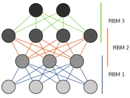
2.7 Deep Belief Network . . . 28

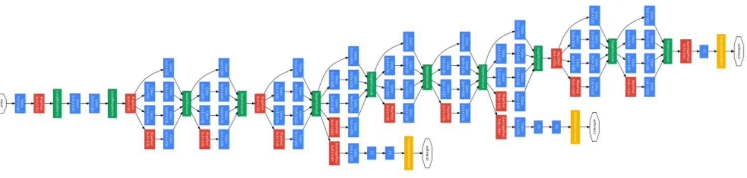
2.8 GoogLeNet with 2 intermediate and one final outputs. . . 29

3.1 Motion History Image on silhouette with various decay rates� . . . 38

3.2 Sample annotations for the Montalbano v2 dataset. . . 40

3.3 Sample frames, depth maps and body pose coordinates . . . 40

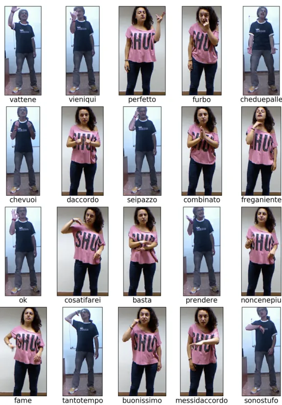
3.4 Classes from the Montalbano v2 dataset . . . 42

3.5 Histogram of the gesture instance durations . . . 43

3.6 Sample transformations and augmentations on image frames. . . 43

3.7 Typical features extracted from the body pose coordinates . . . 44

3.8 Hand crops used as image features . . . 45

3.9 Experimental setup with one shared representation learning path and the Hy-brid NN-HMM or the BDRNN model . . . 46

3.10 Architecture of the embedding models Neural Networks. . . 48

3.11 Wide ResNet Neural Network in 16-1 configuration . . . 49

3.12 HMM State transitions model . . . 50

3.13 Number of frame occurrences by class in the Montalbano v2 dataset . . . 52

3.14 Posterior state probabilities over time. . . 54

3.15 Sample predictions from the BDRNN model on body pose data. . . 55

3.16 Accuracy during gestures discriminated by the duration of the detection. . . . 55

3.17 Difference between the confusion matrices . . . 60

3.18 Confusion matrices for BDRNN model . . . 62

3.19 Pairs of samples from easily confused classes . . . 63

(14)

LIST OF FIGURES

3.20 Histogram of sequence-wise Jaccard Index scores . . . . 64

3.21 Distribution of delays between predicted and annotated gesture boundaries. . 64

3.22 Color coded accuracy within annotated gesture boundaries. . . 65

3.23 Distribution of delays between predicted and annotated gesture boundaries. . 65

3.24 HMM State transition probabilities . . . 66

3.25 State posterior confusion matrix . . . 67

3.26 Temporal Convolution layer. . . 69

3.27 Rows from the Temporal Convolution filters in the body pose BD-RNN model. 70 3.28 Jaccard Index over the validation set under varying temporal context sizes. . . 72

3.29 Filters from a Temporal Convolution layer with mono-directional RNN based model. . . 73

3.30 Main steps and models architecture for transfer learning experiment . . . 75

4.1 Siamese Neural Networks for binary verification . . . 85

4.2 Meta-Learning with sequential episodes [Hochreiter et al., 2001] . . . 88

4.3 Sample crops of the subject from the DEVISIGN dataset . . . 92

4.4 RNN-based sequence embedding function from [Pei et al., 2016] . . . 94

4.5 Architecture of the embedding Neural Network . . . 95

4.6 Distributions of embedding neurons activations during the initial training iter-ations. . . 96

4.7 Limitations of Contrastive Loss . . . 97

4.8 Histogram of cross entropy losses on training sequences. . . 100

4.9 similar gestures in DEVISIGN . . . 102

4.10 Pseudo confusion matrix . . . 103

4.11 Accuracy under varying episode vocabulary sizes and training shots . . . 104

4.12 Performances on crossed training/testing difficulty levels . . . 105

4.13 Matching Networks. . . 106 B.6 Architecture de l’extracteur de représentations pour l’apprentissage one-shot. 145

(15)

List of Tables

2.1 Notations . . . 11

3.1 Accuracy and Jaccard Index metrics with body pose features . . . 59

3.2 Accuracy and Jaccard Index metrics with hand crops video input . . . 61

3.3 Accuracy and Jaccard Index metrics on various modalities. . . 68

3.4 Performance metrics in transfer learning experiments. . . 76

3.5 Performance metrics for the BDRNN trained over posterior state probabilities. 77 4.1 Accuracy and target rank for 20 class vocabulary experiments. . . 101

4.2 One-Shot Learning with Matching Networks . . . 108

(16)

(17)

Chapter 1 Introduction

Over the last 50 years, the volume of interaction between humans, computers and the rest of the world has expanded immensely. Long gone is the time of physical terminals where a two-ways textual communication with instructions and feedback gave access to what could be summarized as a general purpose automaton. With diverse sensors, actuators, and increased computation power, computers have found uncountable applications in most domains of human activity. One fascinating branch of this expansion is Machine Learning, whose purpose is to equip computers with somewhat generic models capable to learn and generalize from observations like humans do.

Some compelling applications are now available for daily use by the laypeople: speech recog-nition for dictation or virtual assistants, handwriting recogrecog-nition, etc. Furthermore, expert tasks have also integrated machine learning in a wide diversity of domains, for example: medicine with radiography or microscopic image segmentation [Ronneberger et al., 2015], mechanical failure detection with non-invasive railway damage probing [Lee et al., 2016], image de-noising [Lehti-nen et al., 2018], and biometric identification [Taigman et al., 2014].

This thesis focuses on sequential data, in practice a stream or a time series of observations annotated by one or several labels possibly in a sequence as well. There are countless sources of sequential data in our daily activities on which Machine Learning could prove useful: speech, online handwriting, gestures, video recordings of objects, physical quantity measurements, etc. To set a more concrete objective to this thesis, gesture recognition from videos and body poses has been selected as an application example to illustrate and support the studies. The general motivation was to select a task that encompasses multiple modalities of various natures, low and high dimensional, and has a concrete application, in this case a human-computer interface.

The prediction of sequences can take different forms: in the isolated recognition task, a se-quence of temporal observations containing a simple instance of a class is submitted for recog-nition, whereas in the continuous recognition task, the model can be charged to identify the successive instances of different gestures from a stream of input observations with possibly non-gesture segments in between the non-gesture instances. As an additional requirement, one may seek to obtain the temporal alignment of the instances (positioning beginning and end of gestures).

(18)

1.1 Overview of Gesture Recognition

Another realistic setting is the one-shot or few-shot learning paradigm where only one or a few training instances are available for each class. Such a model could potentially learn new classes very quickly. Finally, one can foresee some use for the online learning and incremental learning paradigms for user or task adaptation. To illustrate these settings in a real world environment, one can imagine an industrial robot tasked to execute operations triggered by specific gestures interpreted as instructions. The one-shot learning and incremental learning aspects would help to program the robot for new instructions while the online learning could provide some level of adaptation with the human operator.

1.1 Overview of Gesture Recognition

1.1.1 Motivations

From the universally known gestures such as pointing or waving to the standardized military signs, gestures offers a flexible, practical and almost universal communication support which is encountered daily in our lives. Consequently, it is easy to imagine applications of a recognition system for human-computer interfaces in the line of existing solutions for speech and handwrit-ing. The literature on the topic notably mentions video games [Ibañez et al., 2014], contact-less computer control in medical environment [Jacob and Wachs, 2014] and industrial robot con-trol [Duan et al., 2017] as examples.

From a technical standpoint, recognizing gestures is a fascinating challenge. Indeed, the level of analysis and understanding of gestures is less extensive than in other fields with similar objectives such as handwriting or speech recognition, which explains the need for significant research effort on the modelling task. Moreover, appearance, shape and movement all play a role so that the information about gestures must integrate data sources of widely different structures such as colour video frames, depth maps, body pose...

Continuous Gesture Recognition is generally described as the spotting and recognition of segments carrying a specific meaning within a recorded stream of observations. These segments may contain static poses or dynamic movements of the body, arms, hands, and facial expression from a person who is trying to convey a message. Active communication through gestures naturally implies a certain level of cooperation from the subject: centred position in front of the camera with few or no occlusions, stable recording conditions to some extent without dramatic lighting changes or varying background for example. This is to be distinguished from activity recognition which tries to analyse a scene from a passive recording where the subject(s) need not take into account the presence of a camera or sensors. Typical activities include running, playing basketball, dancing, cooking, eating, observed by a sort of surveillance camera with a large depth of field. While closely related to gesture recognition, activity recognition often proceeds with different time scales, recording environments and needs to bear with additional difficulties resulting from the passive observation of subjects.

(19)

(20)

(21)

1. Introduction

For recognition, the annotations of a dataset should at least contain the list of gestures iden-tified in each recording (or the class for the single instance in isolated recognition). Optionally, annotations may include temporal alignment providing the timestamps bounding each instance of gesture. Those frontier annotations obviously suffer from a certain level uncertainty intro-duced by transitioning movements that do not clearly belong to any class.

1.2 Continuous Recognition of Sequences

From a general perspective, continuous recognition of sequences belongs to the ensemble of classification problems. Formally, the objective is to predict a target y given an observation x. The sequential aspect means that x comes as a sequence of observations x= (x_t)1_≤t≤�where� designates the length of that particular sequence. All observations x_tcontain the same type of data, usually one vector for each source of data or modality. For a large majority of practical cases, the observations are sampled uniformly along a dimension in space or time. As for the labels, three distinct cases arise in practice; first, the simpler isolated recognition task where each sequence bears a single class value y, for example a gesture label. In a more general case, a sequence contain� < � class instances (y_k)1_≤k≤�to detect, for example a spoken word in audio recordings. This formulation is the most commonly studied one in speech and handwriting recognition, as it exonerate the annotators from providing a mapping between observations and targets; the existence of such a mapping is rarely obvious anyway since target instances may overlap or have uncertain frontiers. Moreover, temporal annotations require an unrealistic amount of annotation work for any reasonably large speech or handwriting datasets. Finally, the

continuous recognition task we explore in this thesis corresponds to situations where observation

time-steps y= (y_t)1_≤t≤�map one-to-one with a target label, therefore providing the temporal placement of instances to be detected. To avoid confusion: no hypothesis claims that y_tis fully

determined by the observation at the same time-step x_t, in fact we will analyse the importance of temporal context in details through our experiments.

Besides the inherent challenges posed by classification, this class of problems is subject to additional difficulties. In absence of information about the temporal support related to a given target y_t(the set of observations which explain this particular outcome), one might need to pro-cess a very large section of the input if not the whole sequence to generate a valid prediction. Even under the hypothesis that only nearby time-steps relate to an output, the extent of the sup-port for one class instance might vary from one sample to another and thus requires a model which can deal with inputs of variable size. The two-dimensional pendant of this issue is the recognition of objects at multiple scales in images. A second challenge stems from the dimen-sion of the inputs, since their size essentially grows linearly with the number of time-steps per sequence. Contrary to image datasets where the sample size is determined by the recording de-vice resolution, temporal sequences can have widely varying sizes depending on the durations. To put the dimension issue into perspective: 12 seconds of speech coded as a 26 feature vector every 5ms have the same dimension as an image of 256× 256 pixels.

(22)

1.2 Continuous Recognition of Sequences

Depending on the desired application, a real-time inference constraint might be added, but more realistically the requirement will be relaxed to a constant delay, meaning the model can wait for a certain number of observations past a time-step t before returning a prediction for y_t.

Given the objectives and challenges stated above, a range of models have been conceived for various applications such as speech, handwriting or gesture recognition. It is generally safe to assume these models can be cast under the following pipeline (with different levels of integration between the modules):

Input data aquisition: This part provides a raw stream of observations over time (eg. videos frames, sound amplitude, etc.)

Feature extraction: This stage often comprises a set of basic pre-processing steps (standard-ization, differentiation over time) or more elaborate field-specific transformations (mel-spectrum or fourier transformations for speech, HOG features for RGB images, pose regression on depth maps, tracking, etc.).

With the advances of deep learning, a parametric model (often a Neural Network) can also provide suitable embeddings of the inputs for the upcoming recognition layers of the model. While such embedding functions are generally not fully interpretable, they are selected for their ability to provide semantically aware representations. The embedding should remain invariant to variations of the input data which are not relevant for the recognition task and should structure the representations so as to reflect principles of compositionality, semantic proximity, etc. For example: it is desirable that a characteristic hand shape from a gesture consistently binds to a given embedding vector regardless of the position of the subject in the image and independently of left or right handedness.

Temporal modeling: This part of the model is in charge of capturing any temporal pattern or

temporal structure that may exist in the input. While this thesis will mainly focus on Hid-den Markov Models [Baum and Petrie, 1966] and Recurrent Neural Networks, many other temporal models exist in the literature: Dynamic time warping [Vintsyuk, 1972], Con-ditional Random Fields [Sutton, 2012], Maximum Entropy Markov Models [McCallum et al., 2000] etc.

It should be noted that this stage can be made optional by the means of a prior segmen-tation step which identifies distinct monolithic parts of a sequence. Subsequent classifi-cation steps on these segments do not necessarily involve an explicit temporal model but may simply rely on aggregated statistics, for example Bag of Words representations [Wang et al., 2013].

Classifier: The separation between the temporal model and the classifier is not necessarily

explicit, but a final module should eventually produce the decision about the classes and the temporal alignment of detected segments in the sequence if required. A vast number of models are available for this module but the choice is mainly conditioned by the structure of the temporal model and the desired type of outputs (isolated or continuous predictions, localized segments or simple event enumeration, etc.).

(23)

1. Introduction

Focusing on building a relatively fast and light version of this pipeline, some works for iso-lated recognition have suggested using dynamic time warping (DTW) directly over hand-crafted features and run the comparison against reference prototypes [Li and Greenspan, 2011], there-fore turning the classification into a re-identification task.

To relax the constraint of managing varying sequence durations in the model, several works have contributed to solutions producing representations of fixed size from a sequence by sam-pling a fixed number of key frames [Wanqing Li et al., 2008; Tripathi and Nandi, 2015], an ap-proach that can incidentally provide invariance to execution speed and help control the dimen-sion of the input for the classifier. Another straightforward solution to leverage classifiers for fixed data size is to simply use a sliding window over the input sequence, which, assuming the input window is sufficient to produce a confident decision, can effectively delegate the detection of temporal patterns to the classification module. A noteworthy illustration of this approach for continuous detection of gestures is given by [Neverova et al., 2014], where windows at multiple time-scales are used to quickly increase the context size and add some invariance to execution speed with a moderate computation cost.

Two temporal models are frequently used in state-of-the-art recognition models, Hidden Markov Models (HMM) and Recurrent Neural Networks. Among other similarities, both adopt an infinite recurrent process to model the evolution over time. Nevertheless, we also view these models as characteristic from two different schools of thoughts to solve the same underlying objective.

From a general perspective, HMMs build upon a probabilistic and generative approach fo-cused on the observation data: judicious assumptions are made about the process that governs the environment and lead to these observations. These hypotheses also serve as simplifications which lead to more amenable inference computations within the probabilistic graphical model family. From an adequately designed model, a lot of insight is gained on this underlying process that can in turn help to solve a desired task, in our case continuous gesture recognition. HMMs are based on a combination of an observation model with a transitions model jointly optimized according to the maximum likelihood criterion [Baum and Petrie, 1966; Rabiner, 1989]. They provide a fairly interpretable and flexible class of models giving access to their internals for anal-ysis and tuning guided by expertise acquired in the field. Training and inference can be done ef-ficiently and robustly using dynamic programming. To leverage more complicated observation models, [Bourlard and Morgan, 1990] suggest some alterations to the HMM in order to trade the observation probability with a discriminative model, in practice a Neural Network. While the so-called Hybrid Neural Network Hidden Markov Model (NN-HMM) looses its generative capabilities in the process, the discriminative model is discharged from selecting hypotheses and learning the structure of observations. Those requirements can introduce additional learning effort and limitations that are only necessary to generate sample observations, but not directly relevant to the recognition task.

RNN and more generally Neural Networks proceed with a radically different approach, largely focused on the target task where modelling focuses more on representing data than

(24)

1.3 One-Shot Learning of Gestures

explaining it. Neural Network training revolves around the objective function that models the task in mathematical terms. The objective helps to learn the underlying model of the data as part of its optimization process and successfully does so on a large variety of tasks and data types. Based on the success of Hybrid NN-HMMs, one may wonder why the Recurrent Neural Net-works, which are similar in their structure were not so successful until the last decade. In their vanilla implementation, the recurrent formulation unfortunately causes a rapid attenuation of signal coming from past observations and from the back-propagated error gradient [Hochre-iter, 1998; Pascanu et al., 2013]. To circumvent the issue, [Hochreiter and Schmidhuber, 1997] proposed to replace the standard recurrent neurons with LSTM cells which are gated neurons that can dynamically reduce the apparent depth of the network with respect to time. With addi-tional refinements [Gers et al., 2000; Gers and Schmidhuber, 2001], more appropriate objective functions [Graves et al., 2006, 2013] and increased computation power to train on large datasets, this class of model has eventually reached state-of-the-art performances and seen its popular-ity peak in a wide variety of sequence related problems: speech recognition [Graves and Jaitly, 2014], activity recognition [Donahue et al., 2014], video or image captioning [Xu et al., 2015], translation [Sutskever et al., 2014], etc.

1.3 One-Shot Learning of Gestures

Despite the name, one-shot learning principally formalizes the inference and testing conditions of a recognition model, within which a learning step occupies a predominant aspect. Indeed, this framework stipulates that, given a few samples from classes never seen before, a single instance in the most extreme one-shot case, a model should succeed in learning these classes and recognizing other instances.

How to learn from a few samples admittedly represents the central challenge of this problem. Indeed, traditional methods designed for large datasets representative of all observable variations of classes obviously fail in this setting, and new model and training techniques are needed to learn the most out of few training shots. Growing efforts contribute to bring the benefits of Neural Networks’ robustness and adaptability to a setting with very little information to train-on. Nevertheless, a lot of attention is also invested into preparing the model prior to the one-shot learning session, which is why we view one-one-shot first as a testing paradigm rather than a learning one.

One-shot learning is relevant to gestures in terms of application and usage: one may wish to program home assistants or robots to react after specific gesture based instructions are given, in the same way we already do with voice based activation. Obviously, end-users won’t partici-pate in long and rigorous enrolment campaigns to provide numerous samples of their gesture based order, hence the need for one-shot capability. This thesis focuses on the isolated gesture recognition task, where a few labelled gestures instances is given as isolated data sequences, each from a class never observed before, and the model must correctly classify these gestures in an additional set of test sequences.

(25)

1. Introduction

Compared to a recognition task in the regular paradigm, one-shot learning remains a barely investigated research field as of today. For example, we only found one publication studying Neural Networks with sequential data [Pei et al., 2016]. This is partly due to the difficulty of the task which requires a radically different approach to modelling and learning. However, recent publications [Santoro et al., 2016; Vinyals et al., 2016a] have laid out more precise specifications of the testing methodology, which help clarify the goals to achieve. The field is therefore quickly gaining momentum. Existing learning methods have been extended to accommodate one-shot conditions and new approaches have been developed: transfer learning, multi-task learning, meta-learning [Schmidhuber, 1987], etc.

1.4 Contributions

At the core of this thesis lies the idea to learn and detect sequentially structured patterns, more precisely temporal ones.

The first part of this thesis gathers work on continuous recognition of sequences, a research framework with a long history that has reached end-users in their daily life with speech recog-nition for example. Research on the subject is still very strong and active, pursuing numerous objectives including the expansion to new application fields or data types and the improvement of performances. Rather than focusing on optimization aspects, this work puts more emphasis on the analysis of two state-of-the-art temporal models, namely the Hybrid NN-HMM and Re-current Neural Networks. With their spectacular progress and state-of-the-art performances, the latter have supplanted the former as a de-facto standard for continuous recognition. Yet both models share interesting similarities, a Neural Network based representation learning stage at the input to begin with. They also rely on state based hidden representations internally with dis-crete states and real vectors for the HMM and RNN respectively, and their inference algorithm both involve a recursion of linear transformations followed by a non-linearities. This work aims to inspect more finely the differences and similarities between Hybrid NN-HMM and RNN models using practical and realistic experiments able to demonstrate their advantges and weak-nesses in practice. Gesture data shines for this purpose as it provides a variety of modalities and data representations with different levels of complexity.

Our contributions begin with the creation of a testing framework with a modular design that ensures a fair comparison between the two models while ensuring optimal training and inference conditions for both models. We run tests on a gesture dataset from a former competition with rigorous evaluation methods and compare our work to previous publications. Our design is validated by demonstrating state-of-the-art performances for both models, on body-pose data, video data and a combination thereof.

Following this essential step, we develop a series of studies that analyse and detail influential aspects of the models and training procedures that impact recognition performances. In partic-ular, we propose alterations to the training procedures of both models to take into account and alleviate issues related to imbalanced representation of classes in the dataset.

(26)

1.4 Contributions

Inversely, we perform a detailed post-training analysis of errors and parameter values for each model in order to reveal and explain important properties. Our experiments show that RNN models manage to achieve a good frame-wise accuracy while missing the concept of gesture duration nonetheless, which leads to noisy predictions and suboptimal performances on short gestures.

Although the literature often report Hybrid NN-HMM with inferior results compared to end-to-end RNN models, we show that most of this difference can be bridged by adding sufficient temporal context into the posterior state model. A comparative study is performed to ascertain the role of this context. We observe that RNNs rely very little on that context and feature a great robustness to the variation of input type and quality overall. We further verify this robustness through a series of Transfer Learning experiments that challenge the model with input representations that were not designed for the given model, but are known to contain relevant gesture information. These experiments also reveal that both models learn largely compatible representations of the input data within their respective representation learning stage.

The second part of this thesis concentrates on a different gesture recognition task: one-shot and few-shots learning of isolated gestures. Little work exists on one-shot sequence recognition in general. Our work contributes to this field by proposing a model based on Recurrent Neural Networks, which improves an existing proposition by [Pei et al., 2016] using a more modern and refined architecture. Using this model as a baseline, we propose several improvements by changing the inference method and training objectives. We also report experiments conducted with the Matching Network model [Vinyals et al., 2016b] on our gesture data. This model adopts the meta-learning principle in its design, a very promising area of research for one-shot learning.

(27)

Chapter 2 State of the Art

This chapter will introduce the state-of-the-art models for continuous sequence recognition, with a bias toward our select support application: Gesture Recognition. We first introduce the Hybrid Neural Network - Hidden Markov Model and explain how it can be trained and used for continuous sequence recognition. The same presentation is then provided for the Recurrent Neural Network. Finally, a section is dedicated to an ensemble of recent Neural Network techniques which participate substantially to the performances of our models.

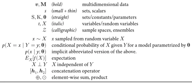
Table 2.1 defines the notations used through this thesis, more specific notations will be intro-duced when needed to facilitate comprehension.

�, � (bold) multidimensional data

s (small + thin) sets, scalars

S, K, � (straight) sets/constants/parameters

t,� (italic) variables/random variables

� (calligraphic) sample spaces, ensembles

x∼ � x sampled from random variable �

p(� = x ∣ � = y; �) conditional probability of � given � for a model parametrized by � p(x ∣ y; �) implicit abbreviated version of the above.

��[f(�)] expectation

� ⟂ � � independent of � [�1, �2] concatenation operator

⊕, ⊙ element-wise sum, product

Table 2.1 –Notations

2.1 Hybrid Neural Network - Hidden Markov Model

In this section, we introduce the Hybrid Neural Network — Hidden Markov Model (NN-HMM). This model is nowadays an industry standard solution for sequence recognition, for example in speech where it comes as a ready-to-use speech recognition module in several software libraries

(28)

2.1 Hybrid Neural Network - Hidden Markov Model

such as CMUSphinx [Lamere et al., 2003] or HTK [Young and Young, 1994]. We will first in-troduce the standard HMM model, then inin-troduce the common design choices for sequence prediction and finally detail the modifications needed to convert it to its hybrid formulation.

2.1.1 Hidden Markov Models: Definition

Hidden Markov Models define a family of Probabilistic Graphical Models for sequences of ob-servations� = (�_t)_t_∈[1..�]with� the length of the sequence. The hidden aspect is brought in by adding series of latent state variables matching the observations at each time step� = (s_t)_t_∈[1..�]. The HMM model is built on the assumption that the hidden states at each time-step govern the associated observations. In probabilistic words, this is enforced by setting a conditional independence of the observations given the latent variables:∀(t, t′), t , t′, �

t ⟂ �t′ ∣ s_t. The

HMM also simplifies the temporal model by enforcing a Markov transition assumption on the states: ∀t, s_t ⟂ (s1, .., st−2) ∣ st−1. The joint probability distribution therefore factorizes over the shared transition and observation models as:

p(�, �) = p(s1)p(�1∣ s1) � ∏

t=2

p(s_t ∣ s_t−1)p(�_t ∣ s_t) (2.1)

For the sake of clarity, we introduce a dummy state variable s0so that the initial state prior

p(s1) can be merged into the product:

p(�, �) =

� ∏

t=1

p(s_t ∣ s_t−1)p(�_t ∣ s_t) (2.2)

The states variables take discrete values in[1 .. K] with K to be defined for the task. It is common to picture those values asK nodes in a graph and imagine that transitions from one state to another correspond to hops from a corresponding node to another. That transition model p(s_t ∣ s_t−1) is governed by a categorical discrete distribution s_t ∼ �at(�_s

t−1) where �i,jis

the probability of the transition from i to j.

To model the observations, many distributions are available; a popular starting point for continuous multidimensional observations such as speech features is often the Gaussian Mixture Model. Without loosing generality regarding the type of observation model, its parameters will be denoted by� for the remaining of this section, leading to the expression of the full joint distribution: p(�, �; �, �) = � ∏ t=1 p(s_t ∣ s_t−1; �)p(�_t ∣ s_t; �) (2.3)

For the sake of clarity, however, the parameters will be omitted in the following of this thesis unless explicitly required.

(29)

2. State of the Art

2.1.2 Hidden Markov Models: Inference and training

Observation likelihood

To calculate the likelihood of a sequence of observations p(�1, .., ��), one needs to eliminate the latent variables from the expression of the joint distribution:

p(�1, .., ��) = ∑ (s1,..,s�)∈[1..K]

�

p(�1, .., ��, s1, .., s�) (2.4) The combinations in the sum above grow exponentially with the length of the sequence rendering the direct naive summation impossible. Instead, a dynamic programming approach breaks the summation in a recurrent way using the forward variable:

�t(i) def

= p(�1, .., �_t, s_t = i) (2.5) which is the probability to reach the state i at time t after generating the first t observations. This variable can take an efficient recursive formulation using the independence assumptions of the HMM: �t+1(j) = p(�1, .., �_t, �_t+1, s_t₊₁= j) (2.6) = p(�t+1 ∣ st+1 = j)p(�1, .., �t, st+1 = j) (2.7) = p(�t+1 ∣ st+1 = j) K ∑ i=1 p(�1, .., �_t, s_t = i, s_t₊₁= j) (2.8) = p(�t+1 ∣ st+1 = j) K ∑ i=1 p(s_t₊₁= j ∣ s_t = i)p(�1, .., �t, st = i) (2.9) �t+1(j) = p(�t+1 ∣ st+1 = j) K ∑ i=1 p(s_t₊₁= j ∣ s_t = i)�_t(i) (2.10) (2.11)

with the initial values�1(j) = p(�1, s1 = j) = p(s1 = j)p(�1|s1 = j) or �0(j) = 1 if a fictional initial state is used. Using this recursion up to t= � takes only �(K2

� ) operations and gives access to the observation likelihood:

p(�1, .., ��) = K ∑

i=1

��(i) (2.12) Maximum-likelihood state assignment: Viterbi algorithm

The Viterbi algorithm is a variation of the previous algorithm for the estimation of the most probable state sequence given a series of observations:

�∗ _{= arg max} �∈[1..K]�

p(�, �) (2.13)

(30)

This is once again resolved through dynamic programming. Let�_t(j) be the probability of the most probable path ending in state j at time t; we note�_t(j) the succession of states in that path, then: �t(j) def = max �1..t−1∈[1..K] t−1p(�1..t−1, st = j, �1..t) (2.14) def = p(�1_..t = �t(j), �1..t) (2.15) = max k∈[1..K] p(st = j ∣ st−1= k)p(xt ∣ st = j) × max �1..t−2∈[1..K]t−2 p(�1..t−2, s_t₋₁= k, �1..t−1) ⏟⏟⏟⏟⏟⏟⏟⏟⏟⏟⏟⏟⏟⏟⏟⏟⏟ �t−1(k) (2.16)

The complete algorithm for the Viterbi maximum likelihood path computation is detailed in Algorithm 2.1. 1: �0(j) = 1, j∈ [1 .. K] 2: �0(j) = [] 3: for t= 1 to � do 4: k= arg max_k′_∈[1..K]�_t−1(k′)p(s_t = j ∣ s_t₋₁ = k′) 5: �_t(j) = [�_t−1(k), j] 6: �_t(j) = �_t−1(k)p(s_t = j ∣ s_t₋₁ = k)p(x_t ∣ s_t = j) 7: end for

8: return��(arg max_k′_∈[1..K]��(k′)) ▷ backtracking

Algorithm 2.1 –Viterbi algorithm

Maximum Likelihood parameters optimization

Since latent variables are present in the model, the maximum likelihood optimization of � and�, the parameters of the observation and transition models, is usually achieved using the Expectation Maximization (EM) scheme, also called Baum-Welch algorithm in that context. The computation in the maximization step also involves dynamic programming methods, this time with an additional backward pass which won’t be detailed here (please refer to [Bishop, 2006] for additional details).

2.1.3 Hybrid Formulation

In this section, we detail how to use Neural Networks to estimate the observation probabilities of the HMM p(�; �). The so-called hybrid implementation of this idea was brought by [Bourlard and Morgan, 1990; Morgan and Bourlard, 1995] and uses the Bayes rule on the observation likelihood p(�_t|s_t) in 2.3 to bring up a predictive state posterior term in the formula:

p(�, �) = � ∏ t=1 p(s_t ∣ s_t−1)p(st ∣ �t)p(�t) p(s_t) (2.17)

(31)

The Bayes rule gives rise to three terms: a categorical distribution of the state priors p(s_t), a prior on the observations p(�_t) which are assumed to be independent identically distributed, and a predictive posterior model of the state probabilities given the observations p(s_t|�_t). In practice, the latter is taken as a Neural Network state classifier with a softmax output interpreted as probabilities.

This modification does not alter the inference algorithms apart from the expansion of the likelihood model into several terms. However, the training procedure now requires to assign values to the states in order to fit the Neural Network parameters and the state priors. Since the states are unobserved variables, it is common to employ yet again an Expectation Maximization, leading to the training procedure described in Algorithm 2.2.

Algorithm 2.2 –Training procedure for Hybrid Neural Network-Hidden Markov

Mod-els.

1: assign arbitrary1state targets ̃y

2: while ̃y not converged do

3: forn epochs do

4: fit state posterior neural network p(s_t = ̃y_t ∣ �_t; �)

5: end for

6: evaluate state priors p(s_t = ̃y_t; �)

7: fit transition model p(s_t₊₁∣ s_t; �)

8: realign ̃y to maximize obs. likelihood for updated model (Viterbi) 9: end while

Two aspects of this algorithm require a special attention:

• Step 4 is a complete Neural Network training procedure by itself with multiple epochs, learning rate schedules, etc.

• The state targets ̃y are solely used to fit the Neural Network. They are not tied to any annotations and solely constrained by the maximum likelihood criterion; as such, the whole training procedure remains unsupervised. In the next section, amendments to this procedure are added to integrate partial supervision.

With the generic elements of the Hybrid NN-HMM introduced along with the training algo-rithm, the final requirement to produce a working recognition system is to elaborate a proper interpretation of the model for the recognition task.

2.1.4 Specialization for Subsequence Detection

Up to this point, the predictive capacity of the Hybrid NN-HMM model has not been mentioned nor have the target annotations been utilized; the training algorithm presented previously only maximizes the likelihood of the observations. Since this work is mostly interested in continuous

1_{A better initialization will reduce the number of training iterations needed. A fairly robust heuristic will be}

presented later on for the semi-supervised version of this algorithm.

(32)

recognition, the objective considered here is to find the boundaries and the label for events within a sequence of observations, or equivalently to classify each observation at each time step in conformance with the annotations, for example: the event might be a word uttered over a few time-steps within a longer recording of a speech; the moment and signification of this word is given during training and must be inferred for prediction.

The approach which is largely used in the literature requires no modification to the HMM model and simply relies on the values of the states to perform the predictions. More precisely each state value is dispatched into one of the classes to be predicted so that given the most likely path through the states for a series of observations, the mapped sequence of labels is also directly available.

The number of states must be at least equal to the number of classes but it is often greater in practice, resulting in multiple states for each class. This apparent redundancy is mostly needed for composite classes built from several elementary units which can be handled by different states. For example the gesture “hello” contains a raising arm motion, an open hand pose and a lowering arm motion which are all very distinct elementary parts of the same class. While the state posterior model could potentially capture all these sub-units into one state, having several distinct ones facilitate learning and lets the transition model learn the interactions that may exist between these states, such as an ordering or a repetition. Besides, expert knowledge and assumptions can be injected more easily into the transition model for simple interpretable concepts: for example one gesture may not transition to another half-way through its execution, therefore many transition probabilities can be zeroed out and excluded from the training process. Figure 2.1 details the typical state structures and assumptions adopted for a speech or gesture recognition transition model [Rabiner and Juang, 1986; Rabiner, 1989].

Now that the model can perform classification, the training procedure needs to be altered so as to maximize the likelihood of the observations subject to predicting the annotated label sequence. Algorithm 2.3 shows the updated training procedure for the Hybrid NN-HMM, modified for supervised learning.

In effect, the states from each class are still realigned but only within the boundaries of each instance of a class as illustrated on Figure 2.2.

(33)

(34)

2.2 Recurrent Neural Networks

1: let(z_t)_t_{∈[1..� ]}be the sequence of labels

2: let m∶ ̃y → ̃z be the state-label mapping function

3: uniformly spread state targets ̃y within annotations ∀1 ≤ t ≤ � , m( ̃y_t) = z_t (refer to Figure 2.2)

4: while ̃y not converged do

5: forn epochs do

6: fit state posterior neural network p(s_t = ̃y_t ∣ �_t; �) 7: end for

8: evaluate state priors p(s_t = ̃y_t; �)

9: fit transition model p(s_t₊₁∣ s_t; �) subj. to chosen hypotheses 10: realign ̃y to maximize likelihood subj. to ∀1 ≤ t ≤ � , m( ̃y_t) = z_t 11: end while

Algorithm 2.3 –Training algorithm for Hybrid Neural Network-Hidden Markov Mod-els.

2.2 Recurrent Neural Networks

2.2.1 Recurrent Neural Networks: Definition

Recurrent Neural Networks (RNN) are a reformulation of the basic feed-forward Neural Net-works which can handle a variable-length sequence of inputs observations(�_t)_t_{∈[1..� ]}:

�t = f(�⊺[�t−1, �t]) (2.18)

where(�_t)_t_{∈[1..� ]} are the hidden state vectors,� are the parameters and f is a non linearity function such as tanh or the sigmoid function. Thanks to the recursive expression, the model itself is invariant through time translation but past inputs are still taken into account via the hidden states. At any given time-step t, recent inputs(�_t−1, �_t−2, … ) affect the value of the hidden state the most in practice, so the hidden states tend to behave as temporally conditioned embeddings of the recent or current inputs. Similarly to a regular feed-forward Neural Network layer, the output of the recurrent layer is composed of the hidden state vectors, a sequence in this case:(�_t)_t_{∈[1..� ]}.

Sometimes, only the final hidden state�� is used because its value is conditioned on all observations and might therefore summarize the information from the whole sequence. This is mostly relevant for non-continuous recognition where the sequence as a whole carries one label. A major advantage of this method is that it maps a variable length input to a fixed size vector which can be more easily fed into a subsequent classifier. However this technique introduces imbalance between the treatment of the first observations, which traverse many layers through time, and the final observations. By contrast, a simple averaging of all hidden vectors gives all time-steps a comparable importance, yet some of the first hidden vectors(�0, �1, … ) might be irrelevant due to the lack of information at this level of progression in the sequence.

(35)

(36)

(37)

(38)

2.3 Recent Advances in Neural Network Training and Architectures

One can compose multiple layers of Bidirectional Neural Networks by stacking them verti-cally over a sequence in order to increase the representational power of the model, in the same fashion as Multilayer Perceptron or Convolutional Neural Networks.

For very long sequences, it can be inconvenient to process a full sequence at once due to mem-ory limitations and large padding overhead if multiple sequences of varying length are batched together (the longest sequence imposes the number of time-steps). Moreover, one may not want to wait for the end of the observation sequence to start reading predictions. Finally, the benefits of the temporal context around any given time-step t are normally limited to a neighbourhood (t − �1, .., t + �2) which can be small in comparison of the sequence duration: �1+ �2 ≪ T. For example, in a full sentence of speech, observations from distant unrelated words most likely cannot help determine the label for the current word. As a result, the Bidirectional Recur-rent Neural Network usually processes a sequence in overlapping chunks of fixed duration: (�1, .., �_c), (�_c−o, .., �2_c−o), (�2_c−2o, .., �2_c−3o), … where c designates the chunk size and o the overlap. The chunk size c is selected so as to include more context than is presumable necessary. The edges of the outputs sequence are discarded to avoid returning predictions lacking from a sufficient amount of context, while the overlap makes sure that all time-steps of the sequence are eventually mapped to an output in one of the chunks.

Chunking solves all the aforementioned issues by compromising on the size of the temporal context; it caps the memory requirements to a known constant, and lets the model return its out-put within a constant delay since observations beyond the chunk will not influence its outout-put. If the computation speed of the whole model remains sufficiently high and the latency intro-duced by the constant delay is judged negligible, this model can integrate a real-time prediction framework.

2.3 Recent Advances in Neural Network Training

and Architectures

We compile here a series of short presentations for recent major contributions in the field of Neural Networks. Although the core of our work does not focus primarily on designing Neu-ral Network modules and optimizing them, the methods presented in this section contribute noticeably to the performances of our proposed models.

Dropout

Dropout [Srivastava et al., 2014] is a noise based regularizer which disables (sets to zero) a fixed proportion r of the neurons in a layer before applying the non-linearity.

Dropout belongs to the class of regularizers which injects a destructive noise inside the model similarly to gaussian noise regularisation. However, randomly disabling neurons at each train-ing iteration also amounts to temporarily train a different sub-model which contains only the retained neurons and merge it back into the full Network which is a form of model averaging.

(39)

Letℬ denote the Bernoulli distribution. For any neuron with output value ̃h, the noisy output is given by: h =⎧{_⎨ { ⎩ ̃h 1_−r if d∼ ℬ(r) = 0 0 otherwise (2.28)

The denominator scales up the non-dropped activations to preserve the average activation values over a whole layer regardless of the dropout rate r. This correction is needed for validation and testing where r is modified and set to 0.

The dropout rate, that is to say the proportion of disabled units, needs to be optimized for each problem, but rates up to 0.5 are not uncommon.

Rectified Linear Units

Activation functions turn the set of nodes outputs in Neural Networks, which are essentially a set of linear transformations, into a highly complex non-linear parametric function com-posed of multiple elementary blocks. To avoid computational issues and mimic biological neu-rons [Hodgkin and Huxley, 1952], bounded functions with an almost linear behaviour around zero have often been used, for example with the sigmoid or tanh.

More recently, a simpler activation function known as Rectified Linear Units [Maas et al., 2013] has become a de-facto standard for new Neural Network architectures:

�e��(x) = max(0, x) (2.29) �eaky�e��(x) = 0.1 × min(0, x) + max(0, x) (2.30) The leaky version is slightly more robust to the initial conditions during training. Indeed, its small slope onℛ−_{avoids back-propagating zero gradient for neurons which are rarely activated} as it sometimes happens during the first epochs.

Some of the motivations behind this non-linearity include:

• a non-symmetric behaviour which can implement more complex transformations • a faster computation speed

• absence of shrinking or clipping effect on R+→ preservation of the back-propagated training signal

• increased activation sparsity and “dispersion”1[Willmore et al., 2000] • improved performance metrics observed on various problems

1_{property of the activation distribution where input patterns are encoded over many different neurons instead of a}

few characteristic ones.

(40)

2.3 Recent Advances in Neural Network Training and Architectures

Batch Normalization

Batch Normalization [Ioffe and Szegedy, 2015] stems from the observation that gradient updates try to optimize all layers in parallel without taking care of the co-adaptation between them. As a layer learns new patterns, the distribution of its outputs changes therefore impacting sub-sequent layers. To reduce the impact of this shifting behaviour, Batch Normalization inserts a normalization step so as to ensure that the distributions of activations maintains a zero mean and unit standard deviation. The neuron outputs therefore becomes:

∀k, hk= f (

a_k− � [a_k]

√� �� [ak]

) (2.31)

where a_krepresents the activation of the k-th neuron. The expectation and variance are empir-ically estimated on each minibatch during training whereas the correction during testing uses running statistics learnt during the training phase. This transformation is reported to not only accelerate training, its original purpose, but also to introduce some regularisation as well, there-fore reducing the need for more destructive techniques based on noise injection.

Residual Networks

If the “Deep” aspect of Neural Networks has started to gain attention by 2009 [Krizhevsky, 2009], the number of layers in Neural Networks has truly soared with the introduction of gated layers [Srivastava et al., 2015; He et al., 2016]. Their foundational idea is arguably the same as the one introduced earlier for Recurrent Neural Networks with gated units, but this time the gating mechanism happens vertically across stacked layers of multilayer Neural Networks: instead of shorting time-steps as in RNN, gates render individual layers optional or “skippable” here. One proposition of this concept is given by Residual Layers from [He et al., 2016] where each block of a Neural Network proceeds by adding a correction to the output of the previous layer��_instead of performing the usual affine transformation:

�l+1 = �elu (�l⊕ ℬlock(�l)) _(2.32)

where ℬlock contains a few Neural Network layers without the last non-linearity, which is moved after the element-wise summation with the input�l_{. Figure 2.6 provides an equivalent}

graphical representation of the Residual block. When�lock modifies the dimension of the hidden representation, for example with max-pooling or a layer with a different number of output neurons, the short-cut path is replaced with a very simple operation such as a linear transformation that returns compatible outputs.

Residual Networks introduce a short-cut path with little attenuation from the output down to the input layers. As a result, gradient descent is able to train very deep layers without major difficulties, and the original ResNet paper effectively demonstrates the feasibility of a thousand layer model.

(41)