Compressive Sensing and Multichannel Spike Detection for Neuro-Recording Systems

(1)

UNIVERSITÉ DE MONTRÉAL

COMPRESSIVE SENSING AND MULTICHANNEL SPIKE DETECTION FOR NEURO-RECORDING SYSTEMS

NAN LI

DÉPARTEMENT DE GÉNIE ÉLECTRIQUE ÉCOLE POLYTECHNIQUE DE MONTRÉAL

THÈSE PRÉSENTÉE EN VUE DE L’OBTENTION DU DIPLÔME DE PHILOSOPHIAE DOCTOR

(GÉNIE ÉLECTRIQUE) AVRIL 2016

(2)

UNIVERSITÉ DE MONTRÉAL

ÉCOLE POLYTECHNIQUE DE MONTRÉAL

Cette thèse intitulée :

COMPRESSIVE SENSING AND MULTICHANNEL SPIKE DETECTION FOR NEURO-RECORDING SYSTEMS

présentée par : LI Nan

en vue de l’obtention du diplôme de : Philosophiae Doctor a été dûment acceptée par le jury d’examen constitué de :

M. DAVID Jean-Pierre, Ph.D., président

M. SAWAN Mohamad, Ph.D., membre et directeur de recherche M. ZHU Guchuan, Doctorat, membre

(3)

DEDICATION

(4)

ACKNOWLEDGEMENTS

First, I would like to thank my supervisor, Professor Mohamad Sawan for all his support, encouragement and guidance during my Ph.D. research life in Polystim Neurotechnologies Laboratory at Polytechnique Montreal.

I would also like to thank Hicham Semmaoui and Yushan Zheng for their suggestions at the early stage of my Ph.D. research. Their resourceful experience helped me get rid of some unnecessary detours in research.

Thanks are due to four intern students I guided, Rebai Hassen, Fatma Hawary, Ousamah Younoss Soliman and Morgan Osborn, for their hard work to contribute to my research project.

I thank all staff members and colleagues of Polystim Neurotech Lab who helped me during my stay in Polytechnique Montreal. Special thanks are due to the following people for their helps and collaborations: Marie-Yannick Laplante, Rejean Lapage, Jean Bouchard, Arash Moradi, Sami Hached, Zied Koubaa, Md Hasanuzzaman, Bahareh Ghane-Motlagh, Mohamed Zgaren, and Ghazal Nabovati.

I am also grateful for the support from the Canada Research Chair in Smart Medical Devices, the Natural Sciences and Engineering Research Council of Canada, CMC Microsystems and the scholarship from China Scholarship Council.

Finally, I want to express the deepest gratitude to my family for their love and encouragements during my study.

(5)

RÉSUMÉ

Les interfaces cerveau-machines (ICM) sont de plus en plus importantes dans la recherche biomédicale et ses applications, tels que les tests et analyses médicaux en laboratoire, la cérébrologie et le traitement des dysfonctions neuromusculaires. Les ICM en général et les dispositifs d'enregistrement neuronaux, en particulier, dépendent fortement des méthodes de traitement de signaux utilisées pour fournir aux utilisateurs des renseignements sur l’état de diverses fonctions du cerveau. Les dispositifs d'enregistrement neuronaux courants intègrent de nombreux canaux parallèles produisant ainsi une énorme quantité de données. Celles-ci sont difficiles à transmettre, peuvent manquer une information précieuse des signaux enregistrés et limitent la capacité de traitement sur puce. Une amélioration de fonctions de traitement du signal est nécessaire pour s’assurer que les dispositifs d'enregistrements neuronaux peuvent faire face à l'augmentation rapide des exigences de taille de données et de précision requise de traitement. Cette thèse regroupe deux approches principales de traitement du signal - la compression et la réduction de données - pour les dispositifs d'enregistrement neuronaux. Tout d'abord, l’échantillonnage comprimé (AC) pour la compression du signal neuronal a été utilisé. Ceci implique l’usage d’une matrice de mesure déterministe basée sur un partitionnement selon le minimum de la distance Euclidienne ou celle de la distance de Manhattan (MDC). Nous avons comprimé les signaux neuronaux clairsemmés (Sparse) et non-clairsemmés et les avons reconstruit avec une marge d'erreur minimale en utilisant la matrice MDC construite plutôt. La réduction de données provenant de signaux neuronaux requiert la détection et le classement de potentiels d’actions (PA, ou spikes) lesquelles étaient réalisées en se servant de la méthode d’appariement de formes (templates) avec l'inférence bayésienne (Bayesian inference based template matching - BBTM). Par comparaison avec les méthodes fondées sur l'amplitude, sur le niveau d’énergie ou sur l’appariement de formes, la BBTM a une haute précision de détection, en particulier pour les signaux à faible rapport signal-bruit et peut séparer les potentiels d’actions reçus à partir des différents neurones et qui chevauchent. Ainsi, la BBTM peut automatiquement produire les appariements de formes nécessaires avec une complexité de calculs relativement faible.

Enfin, nous avons complété la mise en œuvre d’un système numérique adaptatif de signaux neuronaux en temps réel, regroupant un détecteur de PA et un compresseur de données basé sur

(6)

la technique d’échantiollannage compressé. Nous avons validé les conceptions d’un seul canal et des multicanaux. Comparé aux systèmes actuels d’enregistrement de signaux neuronaux, le système proposé peut efficacement comprimer un grand nombre d’échantillons acquis et reconstruire les signaux originaux avec une petite erreur; en outre, il présente une faible consommation de puissance et possède une petite surface de silicium. Le prototype du système est prometteur pour l'application dans une large gamme d'interfaces d'enregistrement neuronales.

(7)

ABSTRACT

Brain-Machine Interfaces (BMIs) are increasingly important in biomedical research and health care applications, such as medical laboratory tests and analyses, cerebrology, and complementary treatment of neuromuscular disorders. BMIs, and neural recording devices in particular, rely heavily on signal processing methods to provide users with information. Current neural recording devices integrate many parallel channels, which produce a huge amount of data that is difficult to transmit, cannot guarantee the quality of the recorded signals and may limit on-chip signal processing capabilities. An improved signal processing system is needed to ensure that neural recording devices can cope with rapidly increasing data size and accuracy requirements.

This thesis focused on two signal processing approaches – signal compression and reduction – for neural recording devices. First, compressed sensing (CS) was employed for neural signal compression, using a minimum Euclidean or Manhattan distance cluster-based (MDC) deterministic sensing matrix. Sparse and non-sparse neural signals were substantially compressed and later reconstructed with minimal error using the built MDC matrix. Neural signal reduction required spike detection and sorting, which was conducted using a Bayesian inference-based template matching (BBTM) method. Compared with amplitude-based, energy-based, and some other template matching methods, BBTM has high detection accuracy, especially for low signal-to-noise ratio signals, and can separate overlapping spikes acquired from different neurons. In addition, BBTM can automatically generate the needed templates with relatively low system complexity. Finally, a digital online adaptive neural signal processing system, including spike detector and CS-based compressor, was designed. Both single and multi-channel solutions were implemented and evaluated. Compared with the signal processing systems in current use, the proposed signal processing system can efficiently compress a large number of sampled data and recover original signals with a small reconstruction error; also it has low power consumption and a small silicon area. The completed prototype shows considerable promise for application in a wide range of neural recording interfaces.

(8)

LIST OF TABLES

Table 2.1: Performance comparison of five typical state-of-the art neural recording systems ... 12

Table 2.2: Comparison among different neural recording systems ... 14

Table 2.3: Comparison between random and deterministic sensing matrices ... 40

Table 2.4: The signal compression performance of some compressed sensing matrices ... 41

Table 2.5: Comparison of several signal processing systems for neural recording devices ... 43

Table 2.6: Comparison among amplitude-based, energy-based and template matching-based spike detection ... 44

Table 2.7: Comparison of several template matching-based spike detection systems ... 45

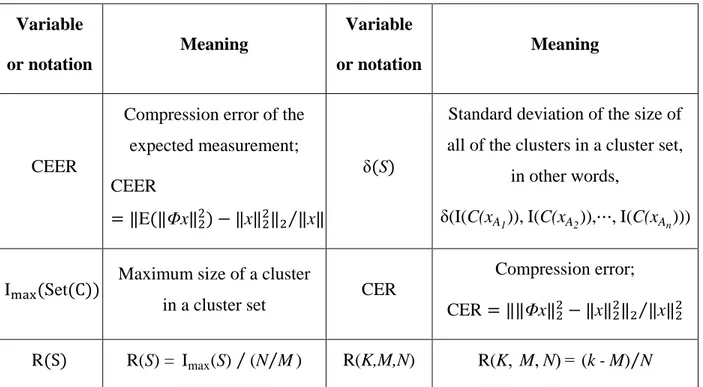
Table 3.1: Symbols and variables ... 53

Table 3.2: Core data clustering algorithm ... 66

Table 3.3: Comparison between the MDC matrix and the other matrices ... 76

Table 4.1: Comparison between the proposed BBTM method and other similar works ... 100

Table 5.1: Detection code of the spike detector ... 115

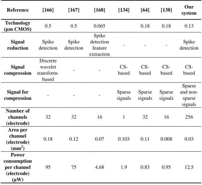
Table 5.2: Comparison of proposed MDC-based digital neural signal processing system with similar existing systems ... 129

Table 6.1: Discussion of contribution of our work comparing with the state-of-the-arts works ... 133

(13)

LIST OF FIGURES

Figure 2-1: A multichannel neural recording system (Polystim) [34] ... 8

Figure 2-2: A typical neural recording BMI [35] ... 9

Figure 2-3: The chopped logarithmic programmable gain amplifier [36] ... 9

Figure 2-4: OTA-C continuous-time delay-filters, (a) the IFLF filter, (b) the cascaded filter [37] ... 10

Figure 2-5: (a) Chip photograph of the proposed nonlinear ADC, (b) power consumption of the chip versus sampling rate (bottom) and spike rate at 200 kS/s (top) [42] ... 10

Figure 2-6: Block diagram of the proposed combined transceivers [45] ... 11

Figure 2-7: Diagram of physiological measurement ... 19

Figure 2-8: Recorded signals from an adult male rhesus macaque monkey ... 21

Figure 2-9: Comparison of four digital estimators, (a) RMS estimator, (b) MAD estimator, (c) Cap fitting estimator, (d) MMS estimator [96] ... 23

Figure 2-10: An analog self-timing static detector [101] ... 23

Figure 2-11: Digital mMMS estimator [102] ... 24

Figure 2-12: Block diagram of STEO-based spike detection with adaptive threshold [90] ... 25

Figure 2-13: Diagram of neural spikes sorting system using TEO spikes detection method [105] ... 25

Figure 2-14: Building blocks synthesizing the TEO-based preprocessor, (a) subthreshold OTA with source degeneration and bump linearization devices, (b) top-level diagram of the TEO preprocessor, (c) the differentiator circuit, (d) four-quadrant analog multiplier [106] ... 26

Figure 2-15: An automatic template matching spike detection method, (a) the proposed template matching spike detection method [112], (b) the Osort algorithm [116] ... 28

Figure 2-16: The spike sorting used to obtain single-unit activity [88] ... 29

Figure 2-17: Block diagram of an integrated neural recording system with spike sorting [59] .... 30

(14)

Figure 2-19: Block diagram of (a) the analog single-channel CS, (b) the digital single-channel

CS [138] ... 31

Figure 2-20: Block diagram of the random modulator [149] ... 34

Figure 2-21: Block diagram of random demodulator pre-integrator (RMPI) [148] ... 35

Figure 2-22: Block diagram of SRMPI [148] ... 35

Figure 2-23: Block diagram of CS encoder [134] ... 36

Figure 2-24: Block diagram of the measurement matrix generation block [134] ... 36

Figure 2-25: Proposed data dictionary based CS system [156] ... 37

Figure 2-26: Proposed CS digital circuit [64] ... 37

Figure 3-1: Comparison between sparsity and similarity. In the simulation, for the core data clustering method, the inner MD is the maximum Manhattan distance between each point to the core data. For the hierarchical clustering, the inner MD is the inconsistency of each cluster (point) under the Euclidean distance. For a signal, 0-MD is the Manhattan distance between a point and the zero. ... 65

Figure 3-2: Relationship between CEER and R(K, M, N). The length of the data is 1000; they are randomly picked from five groups of data, and the process is repeated 100 times. CEER is the compression error of expected measurement. ... 67

Figure 3-3: Relationship between the CER and δ(S) , R(S). Here, N = 1800 and M = 180. δ(S) is the Standard deviation of the size of all of the clusters in a cluster set, and R(K, M, N) = (k - M) / N ... 67

Figure 3-4: Signal reconstruction comparison with the BSBL algorithm: (a) D(K) = 0, (b) D(K) = 0.5 ... 69

Figure 3-5: Signal reconstruction comparison with the BP algorithm: (a) D(K) = 0, (b) D(K) = 0.5 ... 70

Figure 3-6: Signal reconstruction comparison with the OMP algorithm: (a) D(K) = 0, (b) D(K) = 0.5 ... 71

(15)

Figure 3-7: Reconstruction comparison between core data clustering and agglomerative hierarchical clustering with different reconstruction algorithms: (a) block bayesian learning algorithm, (b) basis pursuit algorithm, (c) iterative reweighted least square algorithm, (d) matching pursuit algorithm, (e) iterative threshold-selective projection algorithm, (f) orthogonal matching pursuit algorithm, (g) least absolute shrinkage and selection operator algorithm ... 72 Figure 3-8: Comparison among the data with different length, N = 50 ... 73 Figure 3-9: Comparison between normalized MDC and unit MDC matrices ... 73 Figure 3-10: Comparison of the reconstruction results among sampling rate, compression rate and

reconstruction error under three reconstruction algorithms: (a) BSBL algorithm, (b) BP algorithm, (c) OMP algorithm ... 74 Figure 3-11: Comparison of the reconstruction results of a 600-point non-sparse neural signal

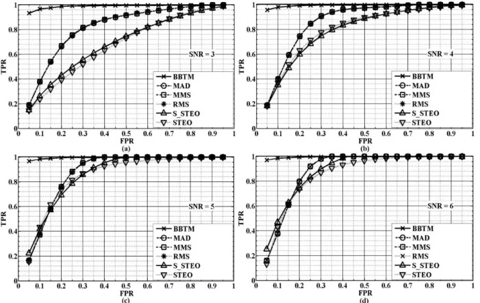
using the UMDC matrix under different CRs, and the reconstruction algorithm is the basis pursuit algorithm: (a) original signal, (b)-(e) are reconstruction results with different CR and (b) CR = 90%, (c) CR = 96%, (d) CR = 98%, (e) CR = 99% ... 77 Figure 4-1: Block diagram of proposed methods (a) BBTM method (b) Osort algorithm ... 86 Figure 4-2: Comparison between BBTM and MAD, MMS, RMS, S_STEO and STEO methods

with firing rate equaling 10, (a) SNR = 3, (b) SNR = 4, (c) SNR = 5, and (d) SNR = 6 ... 90 Figure 4-3: Comparison between BBTM and MAD, MMS, RMS S_STEO and STEO methods

with firing rate equaling 100, (a) SNR = 3, (b) SNR = 4, (c) SNR = 5, and (d) SNR = 6 ... 91 Figure 4-4: BBTM spike detection using MMS to generate spike templates with firing rate

equaling 10, (a) SNR = 3, (b) SNR = 4, (c) SNR = 5, (d) SNR = 6 ... 92 Figure 4-5: BBTM spike detection using MMS to generate spike templates when firing rate

equals 100, (a) SNR = 3, (b) SNR = 4, (c) SNR = 5, and (d) SNR = 6 ... 93 Figure 4-6: BBTM spike detection using STEO to generate spike templates with firing rate

equaling 10, (a) SNR = 3, (b) SNR = 4, (c) SNR = 5, and (d) SNR = 6 ... 94 Figure 4-7: BBTM spike detection using STEO to generate spike templates with firing rate

(16)

Figure 4-8: BBTM spike clustering with MMS-based and STEO-based spike generation methods, (a) SNR = 3, (b) SNR = 4, (c) SNR = 5, (d) SNR = 6 ... 95 Figure 4-9: Research of the threshold control parameters, (a) firing rate is 10 with known

templates, (b) firing rate is 100 with known templates, (c) firing rate is 10 with MMS template generation method when P equals 4, (d) firing rate is 100 with MMS template generation method when P equals 4, (e) firing rate is 10 with MMS template generation method when P equals 5, (f) firing rate is 100 with MMS template generation method when P equals 5 ... 97 Figure 4-10: The results of the generation of the spike templates, (a)-(c) comparison between

original and generated templates with signals SNR equaling 3, (d)-(f) comparison between original and generated templates with signals SNR equaling 6. The red color line is the generated spike templates and the green line is the original spike templates. ... 98 Figure 4-11: The detection results for the signal with SNR equaling 3, (a) original signals, (b) the

spikes in the signal, (c) the detected spikes ... 99 Figure 4-12: The comparison between the classified spikes and the original signals for the signal

with the SNR equaling 3 for three neurons ... 99 Figure 5-1: Simplified diagram of a typical wireless neural monitoring system ... 105 Figure 5-2: Framework of the compressed sensing technique ... 107 Figure 5-3: Diagram of the circuit design using the CS technique: (a) analog design, (b) digital

design, (c) proposed digital circuit design using the MDC matrix ... 110 Figure 5-4: Diagram of the design of digital single-channel circuit ... 114 Figure 5-5: Diagram of the spike detection block ... 115 Figure 5-6: Design of the data compression block: (a) core data clustering algorithm [224], (b)

behavior diagram of the core data clustering algorithm, (c) diagram of the digital circuit of the core data clustering algorithm ... 116 Figure 5-7: Diagram of the multichannel system ... 118

(17)

Figure 5-8: Relation between the distance and reconstruction error, compression rate: (a) relation between the distance and the reconstruction error using BP and Lasso algorithms, (b) relation between the distance and the compression rate ... 120 Figure 5-9: Relationship between the compression rate and the reconstruction error for the

multichannel using: (a) BP algorithm, (b) Lasso algorithm ... 122 Figure 5-10: Relation among channel-to-scan, SNR and reconstruction error rate for the

multichannel processing using: (a) compression rate = 0.5, (b) compression rate = 0.9 ... 123 Figure 5-11: Relation between the scan rate and the power consumption ... 123 Figure 5-12: The comparison between original signals and their reconstructed signals under

different ChS: (a) ChS = 1, (b) ChS = 2, (c) ChS = 4, (d) ChS = 8 ... 125 Figure 5-13: An example of the original signals and their reconstructed signals from 16 channels:

(a) channels 1-4, (b) channels 5-8, (c) channels 9-12, (d) channels 13-16 ... 127 Figure 5-14: The output of the digital circuit: (a) format of the outputs, (b) timing diagram of the

FO and SO, (c) timing diagram of the CO ... 128 Figure 5-15: Post-layout of the proposed 256-channel digital neural signal processing system . 129 Figure 5-16: The FPGA-based simulation: (a) the picture of the FPGA-based test system, (b) FO

(18)

LIST OF ABBREVIATIONS

ADC Analog-to-Digital convertor

AFPR Average false positive rate AP Action potential

ASP Analog signal processing ATPR Average true positive rate

BBTM Bayesian inference based template matching BCH Bose-Chaudhuri-Hocquenghem

BMI Brain machines interface BP Basis pursuit

BSBL Block sparse Bayesian learning algorithm CEER Compression error of the expected measurement CER Compression error

ChS Channel-to-scan parameter

CMOS Complementary metal-oxide semiconductor CS Compressed sensing

CR Compression rate

CRIP Cluster restricted isometry property DD Discrete derivatives

DFT Discrete Fourier transmission DSP Digital signal processing

EC-PC Exponential component–polynomial component ECG Electrocardiography

ECoG Electrocorticography EEG Electroencephalography FM Frequency modulating

fMRI Functional magnetic resonance imaging FPGA Field programmable gate array

(19)

FPR False positive rate

FSDE First and second derivative extrema FSK Frequency shift keying

GLRTs Generalized likelihood ratio test detection IRLS Iterative reweighted least square algorithm Lasso Least absolute shrinkage and selection operator LDPC Low-density parity-check

LRT Likelihood ratio test detection MAD Median absolute deviation MD Maximum distance

MDC Minimum Euclidean or Manhattan distance cluster-based deterministic MEG Magnetoencephalography

MMS Maximum minimum spread sorting

mMMS Modified maximum and minimum spread estimation method MP Matching pursuit

NEO Nonlinear energy operator NIRS Near infrared spectroscopy NMDC Normalized MDC

OMP Orthogonal matching pursuit algorithm OTA Operational transconductance amplifier PRBS Pseudo-random bit sequence

RER Reconstruction error RF Radio frequency

RIP Restricted isometry property RMS Root mean square method

SAR Successive approximation register SD Standard deviation

(20)

SPI Standard series peripheral interface

SR Scan rate

STEO Modified smooth teager energy operator

StOMP Stagewise orthogonal matching pursuit algorithm SWT Stationary wavelet transform

S_STEO Standard smooth teager energy operator TCP Threshold control parameter

TEO Teager energy operator

TDM-FM Time-division-multiplexing, frequency-modulating TPR True positive rate

UMDC Unit MDC

USB Universal serial bus UWB Ultra-wideband VCD Value change dump

(21)

LIST OF APPENDICES

Appendix A – Complementary background on compressed sensing theory………156 Appendix B – Implementation of the front-end circuit……….159 Appendix C – Implementation of the digital signal processing system………164

(22)

CHAPTER 1 INTRODUCTION

1.1 Research Motivation

Brain-machine interfaces (BMIs) have been the subject of a large amount of neuroscientific research since the 1970s [1]. According to the ways of the recording or manipulation, BMIs can be divided into Electroencephalography (EEG), Magnetoencephalography (MEG), Electrocorticography (ECoG), neural recording, Functional magnetic resonance imaging (fMRI), Near infrared spectroscopy (NIRS), etc. Implantable neural recording devices are an important category of the BMIs, which allow researchers to directly acquire signals from single and multiple neuron(s).

Due to the growing sophistication and data collection capacity of neuroscientific research and applications, BMIs need to integrate many functions and process increasingly large amounts of data, which causes that the signal processing becomes an indispensable part. For example, the analysis of EEG signals and fMRI requires feature extraction and classification methods [1] [2]; independent component analysis is used for analysis of MEG signals [3]; Kernel-based learning methods are used to analyse ECoG signals [4]. Designing a real-time adaptive BMI has become a hot topic [5] [6] [7].

Implantable neural recording devices are an important category of BMIs: they allow researchers to directly acquire signals from single and multiple neuron(s). However, an implantable real-time adaptive neural recording device faces many challenges. First of all, it must integrate an ever-increasing number of channels to improve recording performance. The multichannel neural recording system must provide information about neurons at multiple sites and also about the relationship between these neuronal sites. More channels means a huge amount of data must be collected, which presents difficulties in storing, processing and transmitting data to a base station. Also, an implantable device has some challenging design limitations: its surface area should be tiny; it should maintain low temperature in order to protect tissue from heat injury; and it should have low power consumption to permit a long lifetime.

Achieving the fast and accurate neural signal processing needed by an implantable real-time adaptive neural recording device is a similarly challenging goal. Current neural signal processing methods can be divided into two principal strategies: signal reduction and compression. Spike

(23)

detection and sorting are popular signal reduction methods, but despite considerable research, several difficulties remain to be overcome. The first major problem is detection accuracy. The spike detection block should correctly detect all of the spikes while removing the noise, and the detection system should have low complexity to ease its implementation. Furthermore, the spike processing system should separate the overlapping spikes that originate from different neurons. Signal compression can keep the original signal to the maximum possible extent while reducing the burden of the transmission, and therefore it has aroused much interest among designers of neural recording devices [8] [9] [10]. A new signal compression technique called compressed sensing (CS) for use in processing recorded signals has been discussed [11] [12]; however, the neural signal is usually not sparse in the time domain, so the application of the CS technique for neural signals needs further research. Moreover, compressing neural signals requires development of a dedicated sensing matrix with a high compression rate and a low reconstruction error.

Finally, signal processing algorithms should be applied carefully for the circuit design. To date, designers have focused on the design of the front-end circuit and transmitter, but the need to design and develop a high-efficiency, low-cost signal processing system is becoming more and more pressing. The two principal difficulties hindering the development of such a system are the lack of a suitably high-performance and low-complexity signal processing technique, and the non-existence of a circuit design with sufficiently low power consumption.

1.2 Objectives

The main objective of this research was to study new approaches, both in theory and implementation, for spike detection (sorting) and signal compression in a neural recording device. The specific objectives were as follows:

 to develop a sensing matrix for the compression of neural signals using the CS technique;  to understand the process of reconstruction of the original neural signals and determine the

influence of parameters such as the sampling rate and length of the signal;

 to evaluate the high-efficiency spike detection method, including high-accuracy detection and classification of the spikes;

(24)

 to design a digital neural signal processing system that includes spike detection and signal compression, and to test and verify the proposed system.

1.3 Contributions

The contributions of this thesis and our research are summarized as follows:

 New methods about the compression of sparse and non-sparse neural signals with CS technique. A minimum Euclidean or Manhattan distance cluster-based deterministic compressed (MDC) sensing matrix was proposed to compress the neural signal. The MDC can compress sparse and non-sparse signals using the similarity, which is appropriate for the compression of neural signals in the time domain. We also give the mathematic proof of the MDC matrix for compression. Furthermore, the results of our research into other compression methods based on CS technique are outlined.

 New knowledge about the reconstruction of original neural signals with different reconstruction methods. We found that the unit MDC matrix that is composed of zero and one can be used for the compression of neural signals, which has low complexity suitable for the design of the compression system in neural recording devices. The factors that influence the MDC matrix, such as the length of signals, sampling rate, are identified and discussed. The above contributions are detailed in the following published articles:

N. Li and M. Sawan, "Neural signal compression using a minimum Euclidean or Manhattan distance cluster-based deterministic compressed sensing matrix," Biomedical Signal Processing and Control, vol. 19, pp. 44-55, 2015.

H. Semmaoui, N. Li, S. Khayat-Hosseini, J. Martinez-Trujillo, and M. Sawan, "An adaptive recovery method in compressed sensing of extracellular neural recording," Journal of Neurology and Neuroscience, vol. 6(19), pp.1-11, 2015.

 A spike detection and sorting method with a high detection and classification accuracy was proposed; it is based on Bayesian inference-based template matching. Using this system, spikes can be detected with high accuracy, especially for a low signal-to-noise ratio (SNR). Also, the overlapping spikes can be separated and classified. Furthermore, the system can

(25)

automatically generate the templates. Finally, the proposed system has a simple structure which can be used for circuit implementation.

 An amplitude-based thresholding method of spike detection, called modified Maximum and Minimum Spread (mMMS) Estimation Method, was tested. Compared with the original MMS method, mMMS has low power consumption and good detection accuracy for high SNR.

The above contributions are reported in the following articles:

N. Li, H. Semmaoui, and M. Sawan, "Modified Maximum and Minimum Spread estimation method for detection of neural spikes," Proceedings, 2013 IEEE International Conference on Electronics, Circuits, and Systems, pp. 530-533.

N. Li, L. Fang and M. Sawan, "An efficient real-time neural spike detection method based on Bayesian inference with automatic template generation" (under review).

 The design of a neural signal processing system, including spike detection and signal compression, is presented. The design is divided into single-channel and multichannel systems. Based on the single-channel system, the signal processing for a 256-channel multichannel system is discussed. The implemented digital circuit is tested and verified by simulation software and the field-programmable gate array (FPGA) testing board. The proposed system has good processing performance and relatively low power consumption and a small silicon area, which can be used in the neural recording interfaces.

The details of this contribution can be found in the following articles:

N. Li, M. Osborn, G. Wang and M. Sawan, "A Digital multichannel neural signal processing system using compressed sensing technique" Accepted for publication by Elsevier Digital Signal Processing.

N. Li and M. Sawan, "High compression rate and efficient spikes detection system using compressed sensing technique for neural signal processing," Proceedings, 7th International IEEE/EMBS Conference on Neural Engineering, 2015, pp. 597-600.

N. Li, M. Osborn, L. Fang and M. Sawan, "Using Template Matching and Compressed Sensing Techniques to Enhance Performance of Spike Detection and Data Compression Systems" Accepted by 2016 IEEE International Symposium on Circuits and Systems.

(26)

1.4 Thesis Organization

This thesis is written in a paper-based format.

Chapter 2 contains a review of BMIs, neural recording systems and neural signal processing. First, it describes BMIs and their uses, and introduces several signal acquisition techniques of BMIs. Neural recording systems are specifically highlighted, and several systems and processing techniques are compared. All the significant related work in neural recording and signal processing techniques is reviewed. This chapter is one part of a review paper being prepared for submission to a high-ranking circuits and systems journal.

A neural signal compression system based on the CS technique is discussed in chapter 3, where a sensing matrix, called a minimum Euclidean or MDC sensing matrix, is introduced. This chapter explores several key points relating to this sensing matrix and proves that the proposed sensing matrix can be used for neural signal compression. This chapter is published in Biomedical Signal Processing and Control (vol. 19, pp. 44-55, 2015).

In Chapter 4, we propose an automatic template generation system using a Bayesian inference-based template matching method for spike detection and classification. This system accurately detects spikes and classifies spikes. The chapter describes the system and its detection and classification accuracy.

A digital online adaptive neural signal processing system, including spike detection and compression, is implemented in chapter 5. The single-channel processing system includes a spike detection block using the RMS method and a compression block using the MDC matrix. Based on the single-channel design, we investigate the signal processing of a multichannel system and present our results. Finally, the system is verified with an FPGA testing board. This chapter will be published in Elsevier Digital Signal Processing.

Chapter 6 contains the general discussion for the thesis, and our conclusions, along with recommendations for future work, are presented in chapter 7.

(27)

CHAPTER 2 STATE OF THE ART OF NEURAL RECORDING

INTERFACES AND NEURAL SIGNAL PROCESSING TECHNIQUES

In this chapter, we begin with a discussion on BMIs, then review neural recording devices. Finally, we review neural signal processing methods, including spike detection and the CS technique for signal compression.

2.1 Brain-Machine Interfaces

Biomedical signals are important information in research on the human physiological processes. Human bodies are made up of many systems, and each system is comprised of several subsystems that carry on numerous physiological processes. These processes are complex phenomena, and their nature and activities can be reflected by various biomedical signals. These signals can be biochemical (in the form of hormones and neurotransmitters), bioelectrical (in the form of action potentials), or physical (in the form of pressure or temperature) [13].

A BMI is a system which enables the acquisition of information about cerebral activity and also permits the brain to control computers or other devices. The human body can interact with the control signals that are generated by such a system. BMIs can improve the quality of life and reduce the cost of daily care for people with restricted mobility and physical disabilities, through linking to external devices such as computers and assistive appliances which respond to patients’ requirements.

The function of a typical BMI contains five consecutive stages: signal capture, preprocessing of the signal, signal processing, transmission or stimulation, and results analysis or evaluation. The signal capture stage collects biomedical signals. The preprocessing stage prepares signals to be more recognizable in order to deal with them most effectively in the following step. The signal processing stage satisfies the BMI user’s specific requirements with respect to the calculation of the acquired signals, such as feature extraction or spike classification. The transmission or stimulation stage either transmits the acquired signals or stimulates organs or tissues. The final step is the analysis of the acquired signals or the evaluation of the stimulation performance.

Two main categories of the neural signals in the brain can be monitored. One is electrophysiological activity, and the other is hemodynamic activity [14]. Currently, most BMI

(28)

devices use electrophysiological activity to acquire information from the brain. This can be done through two approaches: noninvasive methods and invasive methods. The noninvasive method does not involve surgery being performed on a patient to acquire the signals, so it has minimum risk, considerable convenience for research, and makes recruiting participants much easier [15]. The invasive approach requires implantation of the device into a living body, so most invasive BMIs have been tested only in experimental animals [16]. Five approaches to communicating with the human brain – some invasive, some non-invasive –are introduced below.

Magnetoencephalography (MEG) is a noninvasive method that records the brain’s magnetic activity by means of magnetic induction. MEG has the advantage that magnetic fields are rarely distorted by the skull and scalp, unlike electric fields [17]. A disadvantage of this method is the size and the high price of the acquisition [14]. In addition, the accuracy and flexibility of the MEG still needs to be improved [18] [19].

Electroencephalography (EEG) is a noninvasive method which measures the voltage fluctuations in brain activity caused by the flow of electric current due to the synaptic excitations of the dendrites of the neurons. EEG data collection occurs through electrodes placed on the scalp. Because of its simplicity, it is the most widespread neuronal recording method and has many applications; for example, it can be used to monitor epilepsy [20] [21].

Electrocorticography (ECoG) is an invasive method in which electrodes are placed directly on the surface of the brain to record the electrical activity in the region of the cerebral cortex. Compared with EEG, ECoG has good recording resolution, because it bypasses the signal-distorting skull and intermediate tissue; thus it is suitable for the study of activity such as blinks and eye movement [22] [23].

Functional Magnetic Resonance Imaging (fMRI) is a noninvasive method; it uses the electromagnetic fields to detect changes in cerebral blood flow and oxygenation levels during neural activity. fMRI is often used for blood-oxygen-level dependent contrast imaging [24], but is also used in research and treatment monitoring applications for conditions such as epilepsy and language processing deficiencies [25] [26] [27] [28].

Compared with the four signal recording methods described above, a neural recording system has great promise for advancing the understanding of brain function by allowing scientists to directly observe and analyze neural activity during normal animal behavior [29]. A neural

(29)

recording techniques can be divided into single-electrode and multi-electrode recording methods. Single-electrode neural recording was popular until the 1960s [30] [31]. A recording from a single electrode can reveal the characteristics of one or a few cell(s), but it cannot give information about how neurons networks work together to process information, which requires the use of arrays of microelectrodes to study temporal and spatial relationships between groups of neurons [32]. Therefore, single-electrode recording was eventually replaced by multi-electrode recording.

The first multi-electrode system was proposed by Marg and Adams in 1967 [33]. Since then, multi-electrode or multichannel systems have become mainstream in the neural recording field. Multichannel neural recording reveals the importance of observing the activity and interaction of many neurons simultaneously [32]. Figure 2.1 shows a typical system used to monitor and record neural signals [34]. This system includes the recording electrodes (or probes), the inner and external signal processing circuits and systems, and the wireless transceiver.

Figure 2.1 A multichannel neural recording system (Polystim) [34]

2.2 Neural Recording Devices

A typical implantable multichannel neural recording BMI contains three key parts: the front end, the signal processor and the signal transmission circuits. Figure 2.2 shows a typical neural recording BMI [35]. In this system, it can be seen clearly that this BMI contains a mixed-signal data acquisition part (front-end part), a spike detector (signal processing part) and the serial bus interface (signal transmission part). Signals are amplified and sampled in the mixed-signal data acquisition part. Then the system detects the neural spikes in the digital part. Finally, the

(30)

digitized data points are transmitted through the serial bus interface.

Figure 2.2 A typical neural recording BMI [35]

Generally speaking, the front-end circuit contains two parts: a signal preprocessor and an analog-to-digital converter (ADC). The signal preprocessor includes a signal amplifier and a filter. For example, Figure 2.3 shows a high-pass amplifier that provides a fixed gain of 50 dB and cut-off for all EEG signals with frequencies lower than 0.1 Hz, and power consumption of 99 μW [36]. Figure 2.4 shows a continuous-time OTA-capacitor (OTA-C) filter featuring 9th-order equiripple transfer functions with a constant group delay; the power consumption of this filter is only 360 nW [37]. Recent research, [38] introduced an 800 nW 43 nV/pHz neural recording amplifier using 0.18 μm CMOS technology with an area of 0.05 mm2. Many recent articles concern the design of low-power high-performance amplifiers and filters [39] [40] [41].

Figure 2.3 The chopped logarithmic programmable gain amplifier [36]

An ADC is needed for digitalized calculation and transmission. Figure 2.5 shows a nonlinear signal-specific ADC. Its sampling rate is 25 kS/s and its power consumption is only 87.2 μW

(31)

[42]. Other recent research outputs, [43] [44] contain details of the design of a high-performance ADC.

Figure 2.4 OTA-C continuous-time delay-filters, (a) the IFLF filter, (b) the cascaded filter [37]

Figure 2.5 (a) Chip photograph of the proposed nonlinear ADC, (b) power consumption of the chip versus sampling rate (bottom) and spike rate at 200 kS/s (top) [42]

The second necessary component of an implantable neural recording BMI is the transceiver, and example of which is shown in Figure 2.6 [45]. This transmitter has a 1 GHz frequency band and a 20 Mb/s transmission rate. The power consumption of this transmitter is only 4.8 μW with a

(32)

0.9 V power supply. More information about the design of transceivers can be found from references [46] [47] [48].

Figure 2.6 Block diagram of the proposed combined transceivers [45]

Thirdly, in a neural recording BMI, the signal processor is a very important part. It enables spike detection [29], feature extraction [49], and data compression [10] [50]. Spikes in brain activity can be used to study epilepsy [21] [51] ; in a typical epilepsy system, spikes detection is the first step in feature extraction [52]. In addition, spike detection can be used to study the activity of the neurons of the prefrontal cortex [53] [54] [55] [56]. Currently, most existing neural recording or stimulation systems integrate a spike detection function [57].

Although the literature on this topic is large, we focused on a comparison of the most recently published neural recording systems, which are not merely front-end but include detection, compression and transceiver circuits, or all of these. We describe five typical state-of-the-art neural recording systems in Table 2.1, and compare other systems outlined in articles published from 2007 to 2015 in Table 2.2. One system introduced in reference [58] is based on the analog-spike detector, and reference [59] introduces a system that uses only digital methods for signal processing. Two neural recording systems in references [54] and [60] use analog and digital methods to reduce or compress signals. The system described in [47] does not include signal processing.

(33)

Table 2.1 Performance comparison of five typical state-of-the art neural recording systems Reference [47] [54] [58] [59] [60] Electrodes 10 1 100 128 64 Amplifier Folded cascode OTA Low-noise programmable gain OTA Two-stage OTAs OTAs Two-stage operational amplifier Gain (dB) 40 Adjustable between 47.5 and 65.5 60 60 60

Low and high cut-off frequency (Hz) 300, 8.13k 167, 6.9k 300, 5k 0.1-200 (low-frequency roll-off), 2k-20k (high-frequency roll-off) <10–100, 9.1k

ADC None 8-bit SAR

ADC 10-bit SAR ADC Adjustable 6-bit or 9-bit SAR ADC 8-bit ADC Sampling rate (ksample/s) None 90 15 40 7.8 Signal reduction None Analog detector and feature extraction Analog programmable threshold Nonlinear energy operator and feature extraction Analog spike detector Signal

compression None None None None

Digital data compressor Transmission TDM-FM 433M Hz None FSK transmitter 433M Hz Ultra wideband transmitter FSK transmitter 4M/8M Hz Size (mm) 22 × 11 × 5 0.4 ×0.4 4.7 × 5.9 8.8 × 7.2 14 × 15.5 Power consumption of the system (mW) 5 3.1×10-3 13.5 6 14.4 Process Technology (μm) 0.5 0.18 0.5 0.35 0.5

(34)

Through comparing these neural recording systems, some conclusions can be drawn. First, signal processing systems are important. In the past, most implemented neural recording systems focused on the pre-processing, including the amplifier, filter and analog-to-digital data conversion. Some systems do not include any signal reduction and compression components or may integrate a simple spike detection system. Recently, lots of systems have begun to integrate more complicated signal processing systems, such as spike-sorting systems and CS-based signal compression systems; as noted previously, signal processing systems for neural recording devices have become a hot research topic.

Table 2.1 and Table 2.2 also show that designers are using more electrodes or channels for neural recording systems. Currently, to the best of our knowledge, the maximum number of electrodes used in a neural recording system without wireless telemetry and signals compression is 11,011 [61], which shows that huge numbers of electrodes can be used for a neural recording system, but with the limitations of power and size, the recorded data cannot be transmitted through wirelessly. Therefore, advances in neural signal processing are necessary.

Both analog and digital methods are used for signal processing. The digital method offers higher accuracy than the analog one. For example, for spike detection, the digital method can optimally implement the corresponding detection methods from the mathematical formulas to calculate thresholds, which means that the digital method is “smarter”, more flexible and has higher estimation accuracy [62].

Finally, as previously noted, a neural recording device must have low power consumption and small silicon area. The transmitter of a wireless multichannel implantable neural recording device consumes more energy than a wired device. There are two reasons for this problem. Firstly, huge amounts of data means that the system must use a high carrier frequency for transmission. Secondly, free carrier frequencies, known as ISM bands, are used to transmit the data, which increases the complexity of the transmission system. Conflicts between transmission and circuit performance can only be resolved by designing a low power and small area signal processing system.

(35)

Table 2.2 Comparison among different neural recording systems

Reference [63] [64] [65] [66] [67]

Year 2015 2015 2015 2014 2014

Electrode 12 4 4 32 8

Amplifier OTA Two-stage

amplifier Two-stage amplifier Intan Technologies RHA2132 amplifier chip Operational amplifier Gain (dB) 40, configurable Configurable 230 − 6 k 72 200 55.7 / 50.3(AP), 50.3 / 45.1(LFP) Low and high

cut-off frequency

(Hz)

Configurable None 30k (H) 0.17, 4.5k 0.12 – 3k, 20 – 2k

ADC SAR ADC

(12 bits)

SAR ADC (10 bits)

SAR ADC

(8 bits) AD7980 None

Sampling

rate(ksample/s) 10

3

20 100 31.25 None

Signal

reduction None None

Energy-based MAD, template matching Analog spike detector Signal

compression CS CS None None None

Transmission None None FM/FSK None None

Power consumption (μW) 4.6g lithium battery,70 hours 16 per electrode 8000 None 4.8 per channel Size (mm) 4.5×1.5 0.11 mm2 per electrode 1.5×0.75 29.5 × 43.3 1.5 × 1.5 Process technology (μm) 0.18 0.18 0.5 None 0.18

(36)

Table 2.2 Comparison among different neural recording systems (cont’d) Reference [68] [41] [69] [70] [71] [72] Year 2014 2013 2013 2013 2012 Electrode 4 100 64 1 10 × 10 Amplifier Fully-differential amplifiers

OTA OTA OTA

Capacitive-feedback, folded cascode OTA Gain (dB) 43 – 80 34 – 40 54 – 60 39.6 46

Low and high cut-off frequency

(Hz)

0.1, 2000 432, 5.1k None 0.8, 5.2k 0.1, 7.8k

ADC SAR ADC

(8 bits) SAR ADC (9 bits) SAR ADC (8 bits) Sigma-delta ADC (13 bits) SAR ADCs (12 bits) Sampling rate (ksample/s) 10 – 100 24.5 – 245 20 2000 20 Signal reduction None Analog spike detection Feature

extraction None None

Signal

compression None None None None None

Transmission MICS/ISM-compliant transmitter digital FSK Burst-mode wideband FSK All-digital pulsed ultra wideband Standard series peripheral interface FSK with 3.2/3.8GHz wireless transmitter Power consumption (μW) 1100 1160 16 per electrode 2760 90.6 Size (mm) 8.6 × 9.7 4.5×1.5 4 × 3 11.25 mm 2 5.2 × 4.9 (preamplifier) 2 × 2 (controller) Process technology (μm) 0.13 0.18 0.13 0.6 0.5

(37)

Table 2.2 Comparison among different neural recording systems (cont’d) Reference [73] [74] [75] [76] [77] Year 2012 2012 2011 2011 2011 Electrode 32 14 1 1 16 Amplifier Two-stage, band-pass, low-noise amplifier Low-noise, low-power amplifiers OTA Instrumentation amplifier Commercial acquisition system Gain (dB) 66.5 500 V/V 100 300,500, 900,1300 76

Low and high cut-off frequency (Hz) Adjustable, 9.6k (H) 250, 10k 300, 5.2K None 300 (L) ADC ADS7953 from Texas Instrument (12 bits) SAR ADCs (11 bits) SAR ADC (9 bits) SAR ADC (11 bits) SAR ADC (8 bits) Sampling rate (ksample/s) Maximum 62.5 26.1 11.52 64 or 1024 None Signal reduction Nonlinear energy operator

None None Feature

extraction

Setting threshold Signal

compression None None None

Adaptive sampling None Transmission None RF transmitter with 902-928 MHz carrier frequency 905 MHz FSK transmitter None Manchester coded frequency shit keying 400M carrier frequency Power consumption (μW) None 1230 1.5v silver-oxide batteries, runs 5 hours 30 for ASP 17200 Size (mm) None 2.36 × 1.88 × 0.25 6 × 5 4.6 × 4.5 None Process technology (μm) None 0.35 0.6 and 0.35 0.5 0.5

(38)

Table 2.2 Comparison among different neural recording systems (cont’d) Reference [78] [79] [80] [57] [81] Year 2010 2010 2010 2009 2009 Electrode 64 1 18 10 × 10 16 × 16 Amplifier Low-noise, band-pass pre-amplifier Two-stage low noise OTA Three-stage instrumentati on amplifier User-selectable amplifier OTA Gain (dB) 65 – 83 50 – 80 72 60 48 – 68

Low and high cut-off frequency (Hz) 10, 10k 0.1 – 1k, 8k, adjustable < 1, 200 250, 5k 0.01 – 70, 500 - 5K

ADC SAR ADC

(8 bits) Commercial component TI MSP430 SAR ADC (12 bits) with power-gating SAR ADC (10 bits) Sample-and-hold circuit (8 bits) Sampling rate (ksample/s) 20 20 0.6, maximum is 100 15.7 < 10k Signal reduction Adaptive threshold Adaptive absolute threshold Spectral energy distribution extraction Adaptive threshold None Signal

compression None None None None

Delta compression lower the resolution Transmission Narrowband 400-MHz binary Manchester-coded FSK Power carrier frequency is 13.56MHz. data carrier frequency is 433/915MHz None FSK modulation with carrier frequency 902-928 Hz None Power consumption (μW) 16600 < 4850 9 uJ/ per feature-vector 8000 5040 Size (mm) 3.1 × 2.7 4.9 × 3.3 2.5 x 2.5 5.4 × 4.7 3.5 × 4.5 Process technology (μm) 0.35 0.5 0.18 0.6 0.35

(39)

Table 2.2 Comparison among different neural recording systems (cont’d)

Reference [82] [83] [84] [85] [86]

Year 2009 2008 2008 2007 2007

Electrode 16 32 16 64 16 × 16

Amplifier OTA Low noise OTA

Two-stage voltage amplifier Low noise multiplexed amplifier array OTA Gain (dB) 45.7, 49.3, 53.7 or 60.5 48 39.6 64 48 – 68

Low and high cut-off (Hz) 1, 12K 1, 7k 0.2 – 94, 140 – 8.2k 6 – 1k, 3 – 15k 0.01 – 70, 500 – 5k

ADC SAR ADC

(10 bits) Normal ADC (5 bits, 10 bits) Gm-C incremental ∆Σ ADC (8-12 bits) AD7277 (10 bits) Off-chip ADC Sampling rate (ksample/s) 256 22 < 16 40 10 Signal reduction None Analog spikes detection Analog filtering Digital filters based detection Wavelet decompos-ition Signal

compression None None None None None

Transmission None Bluetooth

Wireless power harvesting and telemetry system USB 2.0 None Power consumption (μW) 60.3 109.58 1800 33 000 5.04 (with-out wavelet processor) Size (mm) 2.5 × 3.3 3 × 3 3 × 3 2.8 × 3.2 (amplifier array) 40 × 60 (FPGA) 4.5 × 3.5 (only interface) Process technology (μm) 0.35 0.6 0.5 0.35 0.35

(40)

2.3 Neural Signal Processing

Signal processing techniques are used for analysis or perception of physiological measurements. The purpose of acquiring physiological signals is to gain insight into the system that produces these signals. As noted above, these signals may be acquired in electrical form. A typical schematic block diagram of physiological measurement is shown in Figure 2.7. Most of the in situ signal processing follows the process in this diagram. First of all, the designer needs to know the physiological process and design the corresponding signal collector. This collector can be the electrodes, the sensor or the chemical indicator. After collection of the signals, these signals need to be translated into electrical signals. Then, an analog preprocessing can amplify the signal or remove noise. After the analog preprocessing, a digitized conversion prepares for the following calculation, transmission or analysis. If a designer uses analog signal processing in the system, then an analog processor will be added before the converter; if the digital signal processing is applied for the system, then a digital processor is integrated after the converter. Finally, the digitized signals are analyzed in a computer.

Figure 2.7 Diagram of physiological measurement

For a multichannel neural recording device, handling the quantity of the recorded data is one of the most difficult problems that must be solved. Designers need to considerably reduce large amounts of data, without degrading the data quality, for easy transfer through wireless transmission. To solve this problem, two strategies can be applied: signal reduction and compression. Signal reduction methods retain most of the information of the signal but remove useless signals; for example, spike detection is a signal reduction method. Signal (or Data) compression methods use one of many possible approaches to acquire a subset of signals, then based on this subset, apply an algorithm to recover the original signals. In the following two

(41)

sections, two processing strategies, spike detection (and sorting) and signal compression, are reviewed.

2.3.1 Spike Detection and Sorting

Neural signals, produced by the neurons in the brain, can be recorded as bioelectrical signals. Bioelectrical signals are one kind of important biomedical signals that reveal the behavior of relevant organs. The basic component of all bioelectrical signals is action potential (AP) [87]. AP is caused by the flow of sodium (Na+), potassium (K+), chloride (Cl-) and other ions moving across every cell membrane [13]. The AP provides information on the nature of physiological activity at the cell level. When a single neuron is stimulated by a neural or external electrical current, it produces APs. Recording an AP requires the isolation of a single neuron, then microelectrodes with tiny tips are used to stimulate the neuron or record the response [87].

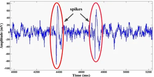
Extracellularly recorded neural signals have some important characteristics. Firstly, extracellularly recorded APs are called spikes [88]. Neurons communicate with each other using spikes. Each spike has an amplitude of about 70 mV (relative to the extracellular fluid) and a duration of around 1 – 2 ms [89] [90]. When an extracellular microelectrode is held tens of microns away from the neurons, a value of 50 – 500 μV can be detected. A typical neuron generates 10 – 100 spikes per second [29] [58]. (Figure 2.8 shows APs collected from multiple neurons of an adult male rhesus macaque monkey). In addition, once a neuron generates an AP, there is a period during which a cell cannot respond to any new stimulation, known as the absolute refractory period (about 1 ms). This is followed by a relative refractory period (several microseconds), and in this period, another AP may be triggered by a stronger stimulation [13]. Spike detection is an important step in many processes and analyses involved in investigating the activity of the nervous system. First, the spike detection process detects APs (spikes) that are immersed in background noise during extracellular recordings of neural signal. This process enables interpretation of neuronal activity and decoding of the included information. Furthermore, spike detection is a very useful reduction process for transmission in a wireless multichannel implantable neural recording system.

Spike detection processing involves two important concepts. The first one is concept of online and offline detection. Online detection means that the neural spikes are detected at the same time

(42)

as the signals are recorded. Offline detection means that detection occurs after recording [88]. This method usually has a long delay, and it is obviously not suitable for a multichannel implantable neural recording system. The second important concept is adaptive detection and the detection of manual setting. The detection of manual setting means that the threshold or template is not calculated from the previously recorded data but is directly set by the designer. In the early days of spike sorting, spike detection was done purely in analog hardware. It was typically performed using a simple voltage trigger, with a voltage threshold set manually by the user [88]. If the voltage of the signal crossed that threshold, a pulse would be generated to indicate the presence of a spike [91]. This method is appealing because of its simplicity, and, as a result, is still used today by many research groups, especially with analog designs [88]. The largest disadvantage of the manual setting method is its requirement for thresholds or templates in advance. In contrast, adaptive detection means that the threshold or template that is used for the detection is determined from the previously recorded data. Comparing with the manual setting method, this method not only runs automatically to detect the spikes but allows estimation of the threshold, which is definitely much more advanced [92]. Currently, neural recording systems usually integrate an online adaptive spike detection component [93] [94] [95]. Furthermore, if the threshold can be acquired in a short time, this method can be called real-time detection [90]. Automatic calculations of the threshold usually involve a training period, and they still can be considered to be real-time processing.

Figure 2.8 Recorded signals from an adult male rhesus macaque monkey

Spike detection techniques can be divided into amplitude-based, energy-based and template matching methods. These methods are described in the following sections.

(43)

2.3.1.1 Amplitude-based Spike Detection

Detecting neural spikes from background noise is commonly done by comparing signals’ amplitudes with thresholds. This method was initially used to analyze offline neural signals [91]. now, amplitude-threshold-based detection is a commonly used online adaptive detection method. The idea of this method is that a spike is a sudden pulse and its amplitude is obviously larger than the ambient signals. The noise of the signal is usually regarded as the Gaussian white noise, and the threshold is the standard deviation multiplied by a coefficient [96]. Based on this idea, several real-time, adaptive spike detection methods are emerging, such as RMS methods [97], median absolute deviation (MAD) [98], EC-PC [99], cap fitting [100], and maximum and minimum spread (MMS) estimation [96] methods. The RMS estimator is traditionally used to estimate the standard deviation of the background noise, which is shown in Figure 2.9(a) [97]. The threshold is calculated using (2.1). 𝑇𝑇 = 𝑃𝑃 × �1 𝑁𝑁� (𝑥𝑥𝑛𝑛− 𝑥𝑥̅) 𝑁𝑁 1 2 𝑛𝑛 = 1. . . 𝑁𝑁 (2.1) where x is the mean value.

The second method is called MAD estimator, which is shown in Figure 2.9(b) [98]. The threshold is calculated in (2.2).

𝑇𝑇 = 𝑃𝑃 ×𝑚𝑚𝑚𝑚𝑚𝑚𝑚𝑚𝑚𝑚𝑛𝑛(|𝑥𝑥𝑛𝑛−𝑥𝑥̅|)

0.6745 𝑛𝑛 = 1. . . 𝑁𝑁 (2.2)

All the samples in a given time frame are subtracted by their mean value. Then the absolute values of the subtracted samples are sorted. The MAD is defined as the median value of |𝑥𝑥_𝑛𝑛− 𝑥𝑥̅|. The standard deviation of background noises is equivalent to the MAD divided by 0.6745.

The next estimator, shown in Figure 2.9(c), is the cap fitting estimator [77]. The threshold T is set as 𝑃𝑃 × 𝜎𝜎, where 𝜎𝜎 is the standard deviation. If T exceeds X0.9987, the distribution of data below T

is considered to be Gaussian noise. Otherwise, the samples that exceed T are regarded as neural spikes and are removed from the signal.

The final estimator, shown in Figure 2.9(d), is the MMS sorting estimator. This estimator has been proven to have better performance than the other three estimators [96]. This method firstly finds the maximum and minimum value of the data during a given time frame (called a window). Then the difference between maximum and minimum value is calculated and stored in a buffer.

(44)

When the buffer is full, all of the data are sorted, and a subset of the sorted data is averaged. Finally, the averaged value is multiplied by an amplification coefficient.

The threshold estimator can be designed as an analog or a digital circuit. An analog self-time static spike detector is shown in Figure 2.10 [101], and a digital spike detector, called an mMMS sorting estimator, is shown in Figure 2.11 [102].

Figure 2.9 Comparison of four digital estimators, (a) RMS estimator, (b) MAD estimator, (c) Cap fitting estimator, (d) MMS estimator [96]

(45)

Figure 2.11 Digital mMMS estimator [102] 2.3.1.2 Energy-based Spike Detection

The energy-threshold-based spike detection method is based on the idea that when a spike happens, the energy of the signal has a sudden change, so the system can calculate the threshold of the change in its energy. An important form of the energy-threshold-based spike detection method is called teager energy operator (TEO) or nonlinear energy operator (NEO) [103]. When the signal is processed in a time-domain or frequency-domain window based on the TEO, this method is called the smooth TEO (STEO), which has better estimation accuracy than the TEO [103]. Equations for the TEO and STEO are established by (2.3) and (2.4).

𝜓𝜓[𝑥𝑥(𝑛𝑛)] = 𝑥𝑥2_{(𝑛𝑛) − 𝑥𝑥(𝑛𝑛 + 1)𝑥𝑥(𝑛𝑛 − 1) (2.3)}

𝜓𝜓_𝑠𝑠[𝑥𝑥(𝑛𝑛)] = 𝜓𝜓[𝑥𝑥(𝑛𝑛)] ⊗ 𝑤𝑤(𝑛𝑛) (2.4) where ⊗ represents the convolution operator and ( )w n represents the window.

The threshold, given in reference [103], is shown in (2.5). 𝑇𝑇 = 𝐶𝐶1

𝑁𝑁∑𝑁𝑁𝑛𝑛=1𝜓𝜓𝑠𝑠[𝑥𝑥(𝑛𝑛)] (2.5)

where N is the number of samples and C is the scaling factor.

The authors in [90] describe another method to calculate the threshold, which is shown in (2.6) – (2.8). In this article, they chose the Hamming window w_H( )n , having the following value

( ) [0.08,0.54,1,0.54,0.08].

H

(46)

𝑇𝑇_𝜓𝜓_𝑠𝑠 = 𝜇𝜇_𝜓𝜓_𝑠𝑠 + 𝑝𝑝𝜎𝜎_𝜓𝜓_𝑠𝑠 (2.6) 𝜇𝜇_𝜓𝜓_𝑠𝑠 = 2.24(𝑟𝑟_{𝑥𝑥𝑥𝑥}(0) − 𝑟𝑟_{𝑥𝑥𝑥𝑥}(2)) (2.7) s_ψ2_s≈4.8r_xx2(0)+ 0.7r_xx2(1) 4.4 r (2) 0.6 r (3) 9.3 r (0) r (2) 1.2 r (1)4.8 r (3)+ _xx2 + _xx2 − _xx _xx − _xx _xx (2.8) where r m is the autocorrelation of ( )_xx( ) x n at lag m.

Some system or circuit designs are based on the TEO or STEO method. For example, the authors in reference [90] propose a spike detection system based on the STEO method, which is shown in Figure 2.12. In reference [104], the authors give the implementation of the STEO method without threshold estimation. The power consumption of the relevant spike detection module in this article is reported as around 1 μW. Also, some designers use the TEO method to design digital (Figure 2.13) [105] or analog spike detector devices (Figure 2.14) [106].

Figure 2.12 Block diagram of STEO-based spike detection with adaptive threshold [90]

(47)

Figure 2.14 Building blocks synthesizing the TEO-based preprocessor, (a) subthreshold OTA with source degeneration and bump linearization devices, (b) top-level diagram of the TEO preprocessor, (c) the differentiator circuit, (d) four-quadrant analog multiplier [106]

2.3.1.3 Spikes Detection with Template Matching

Template matching finds segments of the signals that are similar to the given spike templates. The template matching method is usually complicated, as it contains a convolution and Fourier transformations. This method needs a priori knowledge of spike templates and requires the user to specify a threshold for similarity. In earlier times, some researchers used Euclidean distance [107] and cross-correlation [108] to detect spikes with known templates. A typical template matching technique is matching filter [109] [110]. The discriminant of the matching filter is shown in (2.9):

𝐷𝐷₁ = 𝑥𝑥_𝑛𝑛𝑇𝑇𝑇𝑇 ≥ λ (2.9) where 𝑥𝑥_𝑛𝑛𝑇𝑇 is one segment of the signal, 𝑇𝑇 is the template and λ is the threshold. Reference [111] uses likelihood ratio detection (LRT) to make the template matching-based detection. The discriminant is shown in (2.10) and (2.11)

𝐷𝐷2 = 𝑥𝑥𝑛𝑛𝑇𝑇𝛴𝛴−1𝑇𝑇 H1 > < H0 𝑙𝑙𝑙𝑙𝑙𝑙𝑃𝑃(𝐻𝐻0)(𝑐𝑐10−𝑐𝑐00) 𝑃𝑃(𝐻𝐻1)(𝑐𝑐01−𝑐𝑐11)≡ 𝜆𝜆 (2.10)