HAL Id: hal-01192711
https://hal-univ-rennes1.archives-ouvertes.fr/hal-01192711
Submitted on 3 Sep 2015
HAL is a multi-disciplinary open access
archive for the deposit and dissemination of
sci-entific research documents, whether they are
pub-lished or not. The documents may come from
teaching and research institutions in France or
abroad, or from public or private research centers.
L’archive ouverte pluridisciplinaire HAL, est
destinée au dépôt et à la diffusion de documents
scientifiques de niveau recherche, publiés ou non,
émanant des établissements d’enseignement et de
recherche français ou étrangers, des laboratoires
publics ou privés.
Three-dimensional foam flow resolved by fast X-ray
tomographic microscopy
Christophe Raufaste, Benjamin Dollet, Kevin Mader, Stéphane Santucci,
Rajmund Mokso
To cite this version:
Christophe Raufaste, Benjamin Dollet, Kevin Mader, Stéphane Santucci, Rajmund Mokso.
Three-dimensional foam flow resolved by fast X-ray tomographic microscopy. EPL - Europhysics Letters,
European Physical Society/EDP Sciences/Società Italiana di Fisica/IOP Publishing, 2015, 111 (3),
pp.38004. �10.1209/0295-5075/111/38004�. �hal-01192711�
C. Raufaste1, B. Dollet2, K. Mader3,4, S. Santucci5 and R. Mokso4
1 Universit´e Nice Sophia Antipolis, CNRS, LPMC, UMR 7336, Parc Valrose, 06100 Nice, France
2 Institut de Physique de Rennes, UMR CNRS 6251, Universit´e de Rennes 1, Campus de Beaulieu, 35042 Rennes Cedex, France
3 Institute for Biomedical Engineering, University and ETH Zurich, Gloriastrasse 35, Zurich, Switzerland 4 Swiss Light Source, Paul Scherrer Institute, Villigen, Switzerland
5 Laboratoire de Physique, ENS Lyon, UMR CNRS 5672, 46 all´ee d’Italie, 69007 Lyon, France
PACS 83.80.Iz – Emulsions and foams
Abstract – Adapting fast tomographic microscopy, we managed to capture the evolution of the local structure of the bubble network of a 3D foam flowing around a sphere. As for the 2D foam flow around a circular obstacle, we observed an axisymmetric velocity field with a recirculation zone, and indications of a negative wake downstream the obstacle. The bubble deformations, quantified by a shape tensor, are smaller than in 2D, due to a purely 3D feature: the azimuthal bubble shape variation. Moreover, we were able to detect plastic rearrangements, characterized by the neighbor-swapping of four bubbles. Their spatial structure suggests that rearrangements are triggered when films faces get smaller than a characteristic area.
Foam rheology is an active research topic [1–4],
mo-1
tivated by applications in ore flotation, enhanced oil
re-2
covery, food or cosmetics [5]. Because foams are opaque,
3
imaging their flow in bulk at the bubble scale is
challeng-4
ing. To bypass this difficulty, 2D flows of foams confined
5
as a bubble monolayer, which structure is easy to
visu-6
alize, have been studied. However, the friction induced
7
by the confining plates may lead to specific effects [6],
8
irrelevant for bulk rheology. In 3D, diffusive-wave
spec-9
troscopy has been used to detect plastic rearrangements
10
[7, 8]. These events, called T1s, characterized in 2D by
11
the neighbor swapping of four bubbles in contact, are of
12
key importance for flow rheology, since their combination
13
leads to the plastic flow of foams. Magnetic resonance
14
imaging has also been used to measure the velocity field
15
in 3D [9]. However, both these techniques resolve
nei-16
ther the bubble shape, nor the network of liquid channels
17
(Plateau borders, PBs) within a foam. In contrast, X-ray
18
tomography renders well its local structure. However, the
19
long acquisition time of a tomogram, over a minute until
20
very recently, constituted its main limitation, allowing to
21
study only slow coarsening processes [10, 11].
22
Here, we report the first quantitative study of a 3D
23
foam flow around an obstacle. Such challenge was tackled
24
thanks to a dedicated ultra fast and high resolution imag- 25
ing set-up, recently developed at the TOMCAT beam line 26
of the Swiss Light Source [12]. High resolution tomogram 27
covering a volume of 4.8 × 4.8 × 5.6 mm3with a voxel edge
28
length of 5.3 µm could be acquired in around 0.5 s, al- 29
lowing to follow the evolving structure of the bubbles and 30
PB network. Our image analysis shows that the 3D foam 31
flow around a sphere is qualitatively similar to the 2D flow 32
around a circular obstacle: we reveal an axisymmetric ve- 33
locity field, with a recirculation zone around the sphere in 34
the frame of the foam, and a negative wake downstream 35
the obstacle. Bubble deformations are smaller (in the di- 36
ametral plane along the mean direction of the flow z) than 37
for a 2D flow, thanks to the extra degree of freedom al- 38
lowing an azimuthal deformation: bubbles appear oblate 39
before, and prolate after, the obstacle. Finally, we were 40
able to detect plastic rearrangements, characterized by the 41
neighbor-swapping of four bubbles and the exchange of 42
two four-sided faces. Our observations suggest that those 43
events are triggered when the bubble faces get smaller than 44
a characteristic size around R2
c, given by a cutoff length 45
of the PB Rc' 130 µm in the case of our foam. 46
Experimental set-up – We prepared a foaming solution 47
C. Raufaste et al.
Fig. 1: A plastic bead of 1.5 mm diameter glued to a capillary is placed in the middle of the cylindric chamber of 22 mm diameter and 50 mm height. The acquired tomograms cover the central region with a volume of 4.8 × 4.8 × 5.6 mm3. A typical X-ray projection image is shown on the right.
lauryl ether sulfate (SLES) and 3.4% of cocamidopropyl
49
betaine (CAPB) in mass in ultrapure water; we then
dis-50
solved 0.4% in mass of myristic acid (MAc), by stirring and
51
heating at 60◦C for one hour, and we diluted 20 times this
52
solution. A few mL of solution was poured in the bottom
53
of a cylindrical perspex chamber of diameter 22 mm and
54
height 50 mm. Bubbling air through a needle immersed in
55
this solution, a foam was created until it reached the top
56
of the chamber. The bottom of the cell contains a tube
57
connected to the open air and closed by a tap. Controlling
58
the opening of the tap, we could obtain a slow steady flow
59
of the liquid foam. Its mean velocity determined a
poste-60
riori by image analysis is equal to vflow = 8 µm/s. While
61
flowing, the foam is deformed due to the presence of an
62
obstacle, a smooth plastic bead of diameter 2a = 1.5 mm,
63
attached to a capillary to fix its position in the middle of
64
the chamber (Fig. 1). Because the cell makes a full
rota-65
tion in 0.5 s, the foam experiences centrifugal acceleration,
66
but it remains below 0.5 m/s2within the observation
win-67
dow, hence negligible compared to gravity.
68
The experiments were performed at the TOMCAT
69
beamline of the Swiss Light Source. Filtered
polychro-70
matic X-rays with mean energy of 30 keV were incident
71
on a custom made flow cell (Fig. 1) attached to the
to-72
mography stage with three translational and a rotational
73
degrees of freedom. The X-rays passing through the foam
74
in the chamber were converted to visible light by a 100 µm
75
thick LuAG:Ce and detected by a 12 bit CMOS camera.
76
Typically 550 radiographic projections acquired with 1 ms
77
exposure time at equidistant angular positions of the
sam-78
ple were reconstructed into a 3D volume of 4.8 × 4.8 × 5.6
79
mm3 with isotropic voxel edge length of ps = 5.3 µm.
80
Such a 3D snapshot of the flowing foam is acquired in
81
tscan = 0.55 s, ensuring that motion artifacts are absent
82
since tscan < ps/vflow. In order to follow the structural
83
changes of the foam during its flow around the obstacle,
84
we recorded a tomogram every 35 seconds for
approxi-85
mately 20 minutes (resulting in around 36 tomograms).
86
The tomograms quality is enhanced using not only the
X-87
rays attenuation by the sample, but also the phase shift
88
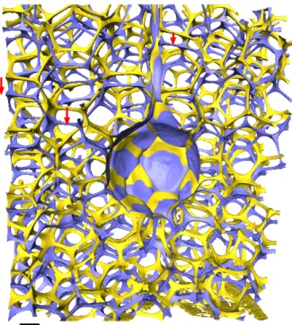
Fig. 2: 3D volume representation of two instances in the foam flow. The PBs and vertices are colored in yellow and blue for time steps t0and t0+35 s respectively. The scale bar is 300 µm.
Red arrows indicate the flow direction.
of the partially coherent X-ray beam as it interacts with 89
the foaming solution in the PBs and senses the electron 90
density variation in the sample [12]. This phase shift was 91
retrieved using a single phase object approximation [14]. 92
Image analysis – The tomograms are then segmented, 93
separating the PBs and vertices from air. Fig. 2 shows 94
two successive time steps of the 3D snapshots of the re- 95
constructed PBs network during the foam flow around 96
the sphere. We measured the liquid fraction from the 97
segmented images, by computing the relative surface oc- 98
cupied by the PBs and vertices on individual horizontal 99
slices. We measured an averaged liquid fraction of 4% over 100
a tomogram, which did not evolve significantly during our 101
experiments. 102
Then, we reconstructed and identified individual bub- 103
bles of the flowing foam, following the procedure we re- 104
cently developed and validated on static foam samples, 105
imaged at the same acquisition rate and spatial resolu- 106
tion [15]. We did not observe any evolution of the size 107
distribution of the polydisperse foam studied here, with 108
an average volume V = 0.36 ± 0.13 mm3, hence
coarsen-109
ing remains negligible. Typically, 160 bubbles are tracked 110
between two successive 3D snapshots, leading to statistics 111
over 5600 bubbles. Bubbles smaller than 0.01 mm3cannot 112
be discriminated from labeling artifacts [15], and thus, are 113
discarded. 114
Velocity field – From the bubble tracking, we could mea- 115
sure their velocity ~V around the obstacle. Statistics are 116
performed in the diametral (ρz) plane of the cylindrical co- 117
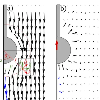
Fig. 3: Velocity fields in the (ρz) plane, (a) in the lab frame. Both the (ρz) or the (rθ) polar coordinates can be used. The unit vectors ( ˆρ, ˆz) or (ˆr, ˆθ) are plotted for r = 1.5 mm in the plane. The normalized velocity field obtained by subtracting the mean flow velocity is shown in (b). The gray half-disc represents the obstacle (diameter 1.5 mm). The red arrow centered on the semi-obstacle gives the velocity scale of 8 µm/s. Blue arrows show the negative wake effect.
depend significantly on the angular coordinate φ (see also
119
below), and we have averaged over this coordinate, as well
120
as over time, thanks to the steadiness of the flow. The
di-121
ametral plane is meshed into rectangular boxes (0.25×0.40
122
mm2). Consistently with the angular averaging procedure,
123
we have checked that the number of bubbles analyzed per
124
box is roughly proportional to the distance of the box
125
to the symmetry axis (data not shown). Averages are
126
weighted by the bubble volumes.
127
The velocity field is plotted in Fig. 3. In average over
128
all patches, the φ-component of the averaged velocity
vec-129
tor is 50 times smaller than its ρz-component, hence the
130
flow is axisymmetric. As expected, the velocity is uniform
131
far from the obstacle, its amplitude decreases close to the
132
leading and trailing points of the sphere, and increases
133
along its sides. Accordingly, there is a clear recirculation
134
zone surrounding the obstacle in the frame of the flowing
135
foam (Fig. 3b). It is worth noting that, compared to 2D
136
foam flows around a circular obstacle [16–19], the range of
137
influence of the obstacle on the flow field is smaller.
138
Interestingly, there is a zone downstream the
obsta-139
cle and close to the symmetry axis where the streamwise
140
velocity component is larger than the mean velocity or,
141
equivalently, where the velocity opposes that of the
ob-142
stacle in the frame of the flowing foam. This reminds
143
the so-called negative wake, revealed in viscoelastic fluids
144
[20–22] and also evidenced in 2D foams [17]. However,
145
a difficulty intrinsic to the 3D axisymmetric geometry is
146
Fig. 4: Velocity components measured at a distance r = 1.5 mm from the obstacle center as a function of the polar angle θ: Vr (blue circles) and Vθ (green squares) in the (rθ) frame.
The lines hold for a potential flow model.
that the statistics is poor in these boxes close to the sym- 147
metry axis (about 10 bubbles per box over the full run), 148
and should be improved in the future. The strong fore-aft 149
asymmetry of the flow evidenced by this negative wake 150
confirms that the foam cannot be modelled as a viscoplas- 151
tic fluid, which gives a fore-aft-symmetric flow [23]: it is 152
intrinsically viscoelastoplastic. 153
To further quantify the velocity field, its components 154
Vr and Vθ at a distance r = 1.5 mm (one obstacle diam- 155
eter) from the obstacle center are plotted as a function 156
of θ in Fig. 4. We have checked that choosing another 157
distance (e.g. r = 2 mm) does not change the qualitative 158
features of the velocity field. The component Vθ is nega- 159
tive, because ˆθ is directed upstream. |Vθ| is maximum at 160
θ = π/2, and Vθ is almost fore-aft symmetric (i.e. sym- 161
metric with respect to the axis θ = π/2). The component 162
Vris positive for θ < π/2, and negative for θ > π/2. Con- 163
trary to Vθ, Vris fore-aft asymmetric. The absolute value 164
of Vr monotonously grows on both sides away from π/2 165
(albeit with noise near 0), it reaches a local extremum 166
near 3π/4 then decreases as θ increases towards π. To 167
further reveal this asymmetry, a comparison is made with 168
a potential flow model, which velocity field writes [24]: 169
Vr = U (1 − r3/a3) cos θ, and Vθ = −U (1 + r3/2a3) sin θ,
170
where U is the uniform velocity far from a spherical obsta- 171
cle of diameter 2a. We proceed as follows: first, we fit Vθ 172
with U as the sole free fitting parameter. This procedure 173
gives the dotted line on Fig. 4, with U = 8.2 µm/s. We 174
then use this value of U in the potential flow formula for 175
Vr, and we plot it as a dashed line in Fig. 4. While Vθ is 176
very similar to the potential flow case (which is expected, 177
since this only tests its fore-aft symmetry), Vr exhibits 178
deviations from potential flow close to θ = 0 and π. In 179
C. Raufaste et al.
Fig. 5: Projection of the bubble deformation field in the (ρz) plane. Ellipses of bubbles are dilated by a factor of 0.5. The colormap gives the amplitude of the normalized deformation in the azimuthal direction.
close to θ = 0, which is a signature of the negative wake.
181
The deviation close to θ = π is more difficult to interpret,
182
and might be due to the presence of the capillary holding
183
the obstacle
184
Bubble deformation – Given the set of coordinates {r}
185
of the voxels inside a bubble, we define its inertia
ten-186
sor I = h(r − hri) ⊗ (r − hri)i, and its shape tensor as
187
S = I1/2. This operation is valid because I (and hence
188
S) is a symmetric and definite tensor. Alike the velocity
189
field, averages are performed inside boxes to obtained a
190
shape field (Fig. 5). The bubble deformation is
quan-191
tified by the eigenvectors/values of the shape tensor. In
192
good approximation, two of them (Sρz+ and Sρz−) are found
193
inside the (ρz) plane, the other corresponds to the
pro-194
jection of the tensor along the azimuthal direction (Sφφ).
195
An effective radius is defined by Reff = (Sρz+S−ρzSφφ)1/3.
196
The bubbles deformation in the (ρz) plane is represented
197
by ellipses of semi-axes S+
ρz and Sρz−. The direction of the
198
largest one, S+
ρz, is emphasized by a line across the
el-199
lipse (Fig. 5). Deformation in the azimuthal direction is
200
quantified by (Sφφ− Reff)/Reff in colormap. The
orienta-201
tion of the ellipses in the (ρz) plane exhibits a clear trend
202
comparable to the 2D case [17, 25]. They are elongated
203
streamwise on the obstacle side and at the trailing edge.
204
In between, the ellipses rotate 180◦ to connect these two
205
regions. We noticed that the deformation of the bubbles is
206
much smaller than for a 2D foam with the same liquid
frac-207
tion [17, 25]. The deformation in the azimuthal direction
208
exhibits dilation/compression up to 5% only. The
quan-209
tity (Sφφ− Reff)/Reff is positive upstream (oblate shape)
210
to favor the passage around the obstacle (Fig. 5). The
211
third dimension tends therefore to reduce the bubble
de-212
formation in the (ρz) plane by increasing the deformation
213
in the azimuthal direction. This effect is opposite
down-214
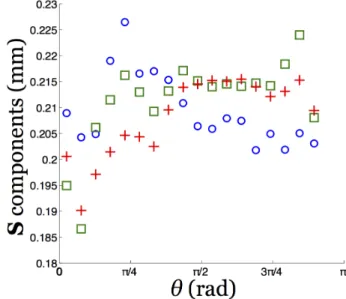
Fig. 6: Shape components measured at a distance r = 1.5 mm from the obstacle center as a function of the polar angle θ: Srr
(blue circles), Sθθ(green squares) and Sφφ (red crosses) in the
(rθφ) frame. The Srθ component is approximately 100 times
smaller than the other components and is not displayed.
stream, right after the obstacle, where the bubbles are 215
prolate. 216
These features are further quantified by plotting the 217
normal components of the shape tensor Srr, Sθθ and Sφφ 218
as a function of θ at r = 1.5 mm, in Fig. 6. This graph 219
shows that these normal components remain within a nar- 220
row range, between 0.19 mm and 0.22 mm, confirming 221
that the bubbles are weakly deformed. These values cor- 222
respond to the typical bubble size. For θ > π/2 (i.e. up- 223
stream the obstacle), Srr is lower than Sθθand Sφφ, which 224
are approximately equal: hence, the bubbles are squashed 225
against the obstacle. Conversely, for θ < 1.2 rad, Srr is 226
larger than Sθθ and Sφφ: the bubbles are stretched away 227
from the obstacle. Hence, close to the axis θ = 0, the bub- 228
bles are elongated streamwise more than spanwise. The 229
origin of the negative wake then becomes clear: by elas- 230
tically relaxing this deformation, the bubbles “push” the 231
streamlines away from the axis θ = 0. Hence, the velocity 232
has to decrease towards its limiting value U as the bubbles 233
are advected away from the obstacle. 234
Plastic rearrangements – Automated tracking of bub- 235
ble rearrangements was hindered by the high sensitivity 236
of such procedure to small defects in the reconstruction 237
of the bubble topology. Description of the contact be- 238
tween bubbles requires to rebuild precisely the faces be- 239
tween bubbles, which would require a finer analysis [26]. 240
Nevertheless, we managed to detect manually four individ- 241
ual events, corresponding to the rearrangements of neigh- 242
boring bubbles. We provide below a detailed descrip- 243
tion of one typical example (Fig. 7); the features of the 244
three other ones were found to be the same. Those re- 245
arrangements consist of the swapping of four neighboring 246
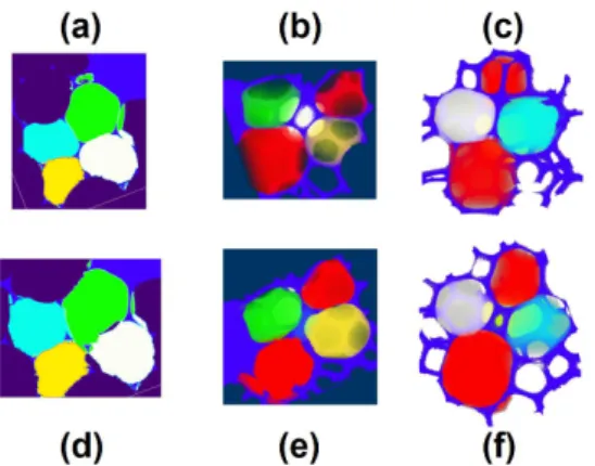
Fig. 7: Example of a T1 in 3D. The white and cyan bubbles lose contact, whereas the green and yellow bubbles come into contact. The red bubbles are the two bubbles that are in con-tact with these four bubbles over the rearrangement. Three different projections are shown: across the four bubbles that swap neighbors, (a) before and (d) after the T1; (b) in the plane of the face that is about to disappear, and (e) in this plane after the T1; (c) in the plane of the face that is about to appear and (f) in this plane after the T1.
or quadrilateral-quadrilateral (QQ) transitions by Reinelt
248
and Kraynik [27,28]. We did not observe three-sided faces
249
during a T1 as reported by [29]. These are likely highly
250
unstable, transient states which are too short-lived to be
251
captured by tomography. The QQ transitions observed
in-252
volve two bubbles losing one face and two bubbles gaining
253
one face. As can be seen on the projection plane across
254
these four bubbles (Fig. 7a and d), this is analogous to
255
T1s in 2D, which always involve four bubbles, two
los-256
ing one side and two gaining one side. The distance
be-257
tween the two bubbles coming into contact decreases of
258
150 µm, from 1.10 mm before the T1 to 0.95 mm after,
259
while the distance between the two bubbles losing
con-260
tact increases of 200 µm, from 1.03 mm before the T1 to
261
1.23 mm after. We checked that the distances between the
262
other bubbles around this T1 change much less. This
cor-263
roborates the vision of a T1 quite similar as in 2D, acting
264
as a quadrupole in displacement, with most effect on the
265
bubbles in the plane. On the other hand, the variation
266
of shape anisotropy of the bubbles involved in the T1 did
267
not show significant trends.
268
We went further on in the characterization of the spatial
269
structure of those rearrangements. Bubble faces comprise
270
a thin film surrounded by a thick network of PBs and
ver-271
tices. We have observed that the thin film part is usually
272
very small for faces that are about to disappear, or that
273
have just appeared, during a rearrangement. However,
274
due to the finite radius of the PBs and of the finite size
275
of the vertices, the “skeleton” of these faces is not
arbi-276
trarily small. Quantitatively, we measured on the images
277
a PB radius Rc = 130 µm. We also measured the area
278
of the skeleton of the faces on 2D projections along the
279
plane of the faces (we did not observe significantly
non-280
planar faces). We always found skeleton areas larger than
281
observations suggest that there is a cut-off area of the or- 291
der of R2
c below which a face becomes unstable, triggering 292
a rearrangement. 293
In summary, we have provided the first experimental 294
measurement of a 3D time- and space-resolved foam flow 295
measured directly from individual bubble tracking, with 296
novel results on all the essential features of liquid foam 297
mechanics: elasticity, plasticity and flow, through descrip- 298
tions of shape field, T1 events, and velocity field. Such 299
experimental results could be achieved thanks to the re- 300
cent advances of both high resolution and fast X-ray to- 301
mography and quantitative analysis tools. We discovered 302
differences between 2D and 3D flows in that the range of 303
influence of the obstacle on the flow field is smaller in the 304
3D case. The same is true for the deformation of the bub- 305
bles which is much smaller in the 3D case. Perspectives 306
include further refinements of the analysis tools [15, 26], 307
to fully automatize the detection of rearrangements, to 308
increase statistics and to study various geometries. Imag- 309
ing the 3D flow at the bubble scale may shed new light 310
on pending issues on shear localization [9] and nonlocal 311
rheology [33]. 312
∗ ∗ ∗
We thank Gordan Mikuljan from SLS who realized the 313
experimental cells, Marco Stampanoni for supporting this 314
project, the GDR 2983 Mousses et ´Emulsions (CNRS) for 315
supporting travel expenses, Fran¸cois Graner, Gilberto L. 316
Thomas and J´erˆome Lambert for discussions and the Paul 317
Scherrer Institute for granting beam time to perform the 318
experiments. 319
REFERENCES 320
[1] Weaire D. and Hutzler S., The Physics of Foams (Ox- 321
ford University Press) 1999. 322
[2] Cantat I., Cohen-Addad S., Elias F., Graner F., 323
H¨ohler R., Pitois O., Rouyer F. and Saint-Jalmes 324
A., Foams, Structure and Dynamics (Oxford University 325
Press) 2013. 326
[3] Cohen-Addad S. and H¨ohler R. and Pitois O., Annu. 327
Rev. Fluid Mech., 45 (2013) 241. 328
[4] Dollet B. and Raufaste C., C. R. Physique, 15 (2014) 329
731. 330
[5] Stevenson P., Foam Engineering: Fundamentals and 331
Applications (Wiley) 2012. 332
[6] Wang Y., Krishan K. and Dennin M., Phys. Rev. E, 333
C. Raufaste et al.
[7] Durian D. J., Weitz D. A. and Pine D. J., Science,
335
252 (1991) 686.
336
[8] Cohen-Addad S. and H¨ohler R., Phys. Rev. Lett., 86
337
(2001) 4700.
338
[9] Ovarlez G., Krishan K. and Cohen-Addad S.,
Euro-339
phys. Lett., 91 (2010) 68005.
340
[10] Lambert J., Cantat I., Delannay R., Mokso R.,
341
Cloetens P., Glazier J. A. and Graner F., Phys.
342
Rev. Lett., 99 (2007) 058304.
343
[11] Lambert J., Mokso R., Cantat I., Cloetens P.,
344
Glazier J. A., Graner F. and Delannay R., Phys.
345
Rev. Lett., 104 (2010) 248304.
346
[12] Mokso R., Marone F. and Stampanoni M., AIP Conf.
347
Proc., 1234 (2010) 87.
348
[13] Golemanov K., Denkov N. D., Tcholakova S.,
349
Vethamuthu M. and Lips A., Langmuir, 24 (2008)
350
9956.
351
[14] Paganin D., Mayo S. C., Gureyev T. E., Miller P.
352
R. and Wilkins S. W., J. Microsc., 206 (2002) 33.
353
[15] Mader K., Mokso R., Raufaste C., Dollet B.,
San-354
tucci S., Lambert J. and Stampanoni M., Colloids
355
Surf. A, 415 (2012) 230.
356
[16] Raufaste C., Dollet B., Cox S., Jiang Y. and
357
Graner F., Eur. Phys. J. E, 23 (2007) 217.
358
[17] Dollet B. and Graner F., J. Fluid Mech., 585 (2007)
359
181.
360
[18] Marmottant P., Raufaste C. and Graner F., Eur.
361
Phys. J. E, 25 (2008) 371.
362
[19] Cheddadi I., Saramito P., Dollet B., Raufaste C.
363
and Graner F., Eur. Phys. J. E, 34 (2011) 1.
364
[20] Hassager O., Nature, 279 (1979) 402.
365
[21] Arigo M. T. and McKinley G. H., Rheol. Acta, 37
366
(1998) 307.
367
[22] Harlen O. G., J. Non Newtonian Fluid Mech., 109
368
(2002) 411.
369
[23] Beris A. N., Tsamopoulos J. A., Armstrong R. C.
370
and Brown R. A., J. Fluid Mech., 158 (1985) 219.
371
[24] Guyon E., Hulin J. P. and Petit L., Hydrodynamique
372
physique (CNRS ´Editions) 2001.
373
[25] Graner F., Dollet B., Raufaste C. and
Marmot-374
tant P., Eur. Phys. J. E, 25 (2008) 349.
375
[26] Davies I. T., Cox S. J. and Lambert J., Colloids Surf.
376
A, 438 (2013) 33.
377
[27] Reinelt D. A. and Kraynik A. M., J. Fluid Mech., 311
378
(1996) 327.
379
[28] Reinelt D. A. and Kraynik A. M., J. Rheol., 44 (2000)
380
453.
381
[29] Biance A. L., Cohen-Addad S. and H¨ohler R., Soft
382
Matter, 5 (2009) 4672.
383
[30] Princen H. M., J. Colloid Interface Sci., 91 (1983) 160.
384
[31] Khan S. A. and Armstrong R. C., J. Rheol., 33 (1989)
385
881.
386
[32] Cox S. J., Dollet B. and Graner F., Rheol. Acta, 45
387
(2006) 403.
388
[33] Goyon J., Colin A., Ovarlez G., Ajdari A. and
Boc-389
quet L., Nature, 454 (2008) 84.