Applying system dynamics to the product development process

Applying System Dynamics to the Product Development Process by

Nancy Riley Jankowiak

B.S., Materials Science and Engineering Massachusetts Institute of Technology, 1993

Submitted to the System Design and Management Program in Partial Fulfillment of the Requirements for the Degree of

Master of Science in Engineering and Management at the

Massachusetts Institute of Technology February, 2000

0 2000 Nancy Riley Jankowiak. All rights reserved.

MASSACHUSETTS INSTITUTE OF TECHNOLOGY

E

0 12000

oB

LIBRARIES

The author hereby grants to MIT permission to reproduce and to distribute publicly paper and electronic copies of this thesis document in whole or in part.

Signature of Author...

Certified by...

A rp i-~ ~

Accepted by...

System I6esign and Management Program January 11, 2000

...

James H. Hines Senior Lecturer, Sloan School of Management ,- Thesis Supervisor

Thomas E. Kochan George Maverick Bunker Professor of Management Co-Director, System Design and Management Program ...

Paul A. Lagace Professor of Aeronautics & Astronautics and Engineering Systems Co-Director, System Design and Management Program

Applying System Dynamics to the Product Development Process by

Nancy Riley Jankowiak

Submitted to the System Design and Management Program

on January 11, 2000 in Partial Fulfillment of the Requirements for the Degree of Master of Science in Engineering and Management

ABSTRACT

A system dynamics study of the product development process at a given company was conducted. The objective was to determine whether system dynamics could be used to understand and improve the process of product development in this particular setting. A team of experts representing the key departments within the company was assembled and used as a resource throughout the project. A standard system dynamics method was used.

Profitability was identified as the key parameter on which the study should focus. Behavior patterns in the product development process were identified by the team, and hypotheses were developed using causal loop diagramming. System dynamics models were then created using Vensim software. These models were simulated and analyzed to provide insights into the real world system which exists at the company.

Key findings included the identification of the tension between management goals and competitive pressures, the potential side effects of cutting costs by reducing resources, and the importance of productivity and the cost of resources. These insights enhanced the company's understanding of their current process and helped them to develop a more systemic view of their problems. Further work will be required to allow full policies for improving profitability to be formulated and tested. The conclusion of this thesis is that system dynamics can and has helped this company to understand and improve its product development process, and the benefits can be enhanced through further application of these techniques.

Thesis Supervisor: James H. Hines

Acknowledgments

Many people helped to make my pursuit of a masters degree, and my completion of this thesis, possible. I am extremely grateful to all of them.

Special thanks go to Jim Hines for introducing me to system dynamics in his classes, and for guiding this thesis as my advisor. His engaging teachings sparked an interest in system dynamics in me, as in many of my fellow students, that I hope to continue to pursue. Appreciation also goes to his great teaching assistants: Jody House, Leslie Martin, Mary Tolikas, and Paulo Goncalves. I would also like to thank Jim Lyneis, who provided his valuable perspective on system dynamics and its applications in several courses.

Many thanks are owed to the staff of ProductCo. The team of experts which provided the main body of knowledge for this thesis, as well as the many others who gave their thoughts on particular areas, were wonderful resources. I am grateful for their time and patience in working with me on this project. Thank you to my company for sponsoring my participation in the System Design and Management Program. Thanks also to the staff of the SDM Program for their help in negotiating my way through it all.

I am deeply indebted to my classmates in the SDM Program. Their varied perspectives made this a rich and unique learning experience. Their knowledge, friendship, and support have been invaluable.

Most of all, I thank my family. My parents taught me early on that education is the greatest gift that you can give to yourself I have been inspired by them and by my sisters throughout my life. I am

profoundly grateful to my husband Rob for his support of my participation in SDM. Without him, I would never have been able to do it.

Table of Contents

Abstract

3

Acknowledgments

5

Table of Contents

7

Introduction: Profitability and Product Development

9

Research Method

10

The Current State of Affairs

11

The Problem

13

The Basics of System Dynamics

14

Analysis of ProductCo's Problem

19

Variables and Reference Modes

19

Hypothesis One: Pressure to Increase Margins 22 Hypothesis Two: Cost Cutting Through Resource Reduction 36

Putting It Together

66

Exploring Potential Policies 68

Conclusions

69

Future Work

71

References

73

Appendix A: Model Documentation 74

Model for Hypothesis One 74

Introduction: Profitability and Product Development

In a complex and competitive market, companies that design and manufacture products have many issues on which to focus. Quality, time to market, customer needs, new technologies -- these things and many others must be considered in running a successful enterprise. However, in the end what keeps the cycle of designing and releasing new products going is money.

It is often difficult for leaders, especially in large companies, to see what impact their policies and decisions will have on the bottom line. This can be extremely complicated in the product development process, where a decision made today may only show its full ramifications several years in the future. At the company studied in this thesis, management was concerned that their level of profitability was not competitive. They suspected that some of the policies and processes embedded in their product

development cycle were hindering their effcrts to improve profits.

Given the complex nature of the product development process and the difficulty of foreseeing the consequences of many actions, system dynamics appears to be a good tool to apply to this problem. The purpose of this thesis was to determine if system dynamics would be useful in helping managers at this company to see how their policies impact profitability. Further, we hoped to identify leverage points for future policies that would help this company reach its desired profit level.

Research Method

In this project I studied a company, fictionalized here as "ProductCo", which designs and manufactures components that are supplied to other companies. These components are incorporated into the other companies' consumer products.

There are several characteristics of ProductCo which are important to this thesis. The company's components, or "projects", are developed over several years and involve a large number of tasks which are performed mainly by engineers. ProductCo bids on and develops projects for a variety of

consumer product manufacturers within its industry. The level of competition is extremely high overall, although it varies over the various types of products which ProductCo supplies.

All of the research for this thesis was conducted on site at ProductCo. The primary method used was interviews, both one-on-one and in larger group sessions. Quantitative data were also obtained from ProductCo.

A "client" in the upper management of ProductCo was identified at the outset, as well as a small core team which participated throughout the project. The team included representatives from engineering, engineering management, business planning, and manufacturing. This covers the major departments which are involved in developing and building products, as well as estimating costs and determining pricing.

The Current State of Affairs

ProductCo has an established product development process, as well as a system for bidding and accounting for costs of projects. This section gives an overview of these as they existed at the start of this thesis project.

The process begins when a customer comes to ProductCo for a bid on a project to design and supply a particular component. This Request for Quote (RFQ) includes a description of the desired component and a list of the specifications that it must meet, as well as an indication of any governmental regulations that will affect the component. The Marketing and Sales department is responsible for putting together the quote response. They must hold a business case review with top management to ensure that it makes strategic sense for ProductCo to go after this project. Based on the business case and the customer who is requesting the quote, the project is assigned to Category A or Category B.

A Category A project is one that ProductCo views as a "must-win" contract. This may be with an established customer, or with a new customer with which the company strongly desires business. It may also be a project that would fill a particular opening at one of ProductCo's existing facilities. These are pursued more aggressively than Category B projects, which ProductCo would like to win but are not viewed as being as essential to the company's future.

Using the category designation as well as historical information from past projects, Marketing and Sales develops a quote which is submitted to the customer. The quote package includes dollar figures for investment and for price per part once the component is in production (piece price). It also includes a

Statement of Work than indicates specifically what design and engineering services will be provided by ProductCo, and what will be the responsibility of the customer.

There may be some negotiation, and then the customer makes their decision. If the quote is accepted, the resources needed for the project are identified and the team is formed. At this stage, key

subsuppliers, if any, are identified and sourced. The supplier engineers then become members of the project team.

The process used for the actual design of the component varies widely. A component that includes software, for example, has a much different design procedure than a component that is strictly

mechanical. Also, some customers source ProductCo with an entire subsystem, which requires more coordination and control activities than a smaller project might. The customer's own product

development process also has an effect; different customers have different requirements for design reviews, prototype builds, and other deliverables.

The design process can be generalized as a set of tasks that must be performed in order for ProductCo to progress from a clean sheet of paper to a completed and validated product design. A task is defined as the unit of work in this process. Sets of these tasks may add up to activities which include creating drawings using CAD (computer aided design), building prototypes, running CAE (computer aided engineering) simulations, writing software, researching competitive products, and performing testing, among other activities.

It is important to note that during the design process, changes to the initial requirements are often made. This could be due to a request from the customer, or due to factors discovered during the design

process that were not previously known. Depending on the situation, the quoted investment or piece price may be renegotiated.

Once the design is complete and is approved by the customer, ProductCo orders or fabricates any special tooling or facilities that are required to produce the component. This phase may overlap the design phase, where possible, in order to reduce the total time required.

The production parts must be validated through testing and in reviews with the customer. Changes are made to the production tools or processes, if required, in order to a provide parts that meet the customer's specifications and any relevant regulations. Once the production components are fully

approved, the ramp-up to full production can begin. Support is provided at the customer's facility as needed for the first builds of the customer's product.

The Problem

ProductCo is in an extremely competitive industry. Many of its smaller rivals have gone out of business, or have been involved in mergers and takeovers. Until recently, ProductCo had been essentially a captive supplier to a single customer. As it tries to branch out and broaden its customer base, ProductCo feels that it must improve its profit margins in order to survive in this competitive environment

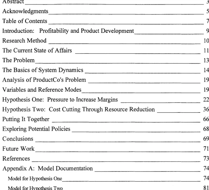
Figure One shows this concem graphically. Profitability, as measured by Return on Sales (ROS), has hovered at a relatively steady level in recent years. ProductCo fears that this level is not high enough to sustain the company; in five years, the company may well be forced to merge or go out of business.

They hope that this can be avoided by finding a way to reach a level of ROS that is comparable to its most successful competitors.

- - - -U

- -

hope

fear

i i

2005

Figure 1: The Problem With Profitability

There are many ways to increase profit. The most obvious is to increase price, though in a competitive environment that may not be advisable. Cost cutting measures may be taken, but they may have unwanted side effects. To help ProductCo evaluate these and other potential policies, I undertook a system dynamics analysis of the problem.

The Basics of System Dynamics

System dynamics is "a powerful method to gain useful insight into situations of dynamic complexity and policy resistance."' That is, we can use it as a tool to help us understand what is going on in the

'Sterman, J. D. 1998. Business Dynamics: Systems Thinking and Modeling for a Complex World. Partial Draft,

Version 1.0, May 1998. Page 1-49.

Profit

(ROS)

1996

1;

NOW

product development process that is affecting profitability, and why actions that we take to improve our situation don't always work as expected.

System dynamics represents the real world system using causal loop diagrams and explicit models with stocks, flows, and information feedback structures. The basic concepts of these tools are presented in this section to aid the reader in understanding the analysis which follows.

Causal loop diagrams are used to represent the linkages between the factors, or variables, in the system. They are often used to show a person or team's dynamic hypothesis -their opinion, based on

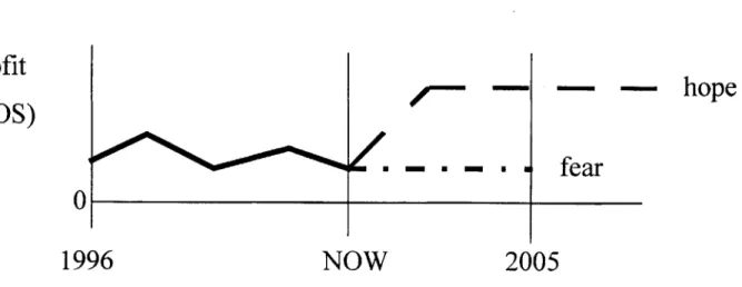
experience, of how a change in one variable drives changes in others. The underlying assumption is that there is feedback in all systems -that is, our actions today influence the situation that will exist in the future. Thus we have causal loops, not causal lines. Figure Two shows a simple example of a loop created by our decisions impacting our environment.

Desi Environ

Actions ed

men Intended Unanticipated

Effects Effects

Environment

In this loop, we take actions based on the current state of our environment as well as the desired state. These actions have effects, which may be as planned or unintentional, that change the state of the

environment and influence our future actions.

The links between variables in a causal loop diagram of a specific system are positive or negative in sign. If, as variable A increases, it causes variable B to increase, there is a positive link from A to B. If, on the other hand, variable B decreases as A increases, there is a negative link from A to B. Examples of these linkages can be observed in Figure Three.

Each loop also has a sign. Positive loops tend to reinforce or amplify whatever is happening in the system, while negative loops counteract and oppose change, seeking to restore balance.2 _{An example}

of each is shown in Figure Three. The sign of a loop can be determined by starting with a change in one variable, tracing the behavior of the variables around the loop, and observing whether it tends to

reinforce the change in the first variable or counteract it. All dynamics in a system are caused by these positive or negative loops, or combinations thereof.

Sales Staff

Budget for

Sales Staff Sales

Revenue +

Number of Rabbits in the

Park

Deaths due to ___ Food

Lack of Food Consumption

Food

Available per _

Rabbit

Figure 3: Positive and Negative Loops

The system can also be represented in a model, using stocks, flows, and information feedback. This is often done after dynamic hypotheses are proposed and diagrammed in causal loops. A simple stock and flow diagram is shown in Figure Four.

Stock z

Inflow Outflow

Auxiliary

Figure 4: Stock and Flow Diagram

Boxes indicate stocks, double arrows with valves indicate rates of flow, single arrows represent information links, and clouds show the boundaries of the model. A variable shown in sharp brackets, such as <variable>, is a shadow variable. This means that it is shown elsewhere in the model; the "shadow" copy allows it to connect back while keeping the diagram neater and more readable.

Each variable has units; for example, a stock might have units of dollars, tasks, items, or some other measurable, while a flow would generally have units of the measurable over time, such as tasks per month.

Underlying the diagram are equations which explicitly state the relationship between each variable. A stock is an integration of all of the rates of flow into or out of it. In the diagram in Figure Four:

T

Stock = Stock0 + f(inf low, -outflow,)dt

0

An information link means that the indicated variables are included in the equation for the variable to which they point. In the diagram in Figure Four, one possibility would be:

Outflow

=

Stock / Auxiliary

This would indicate that the outflow is dependent on the current level of the stock, and some auxiliary which might be the time required to drain the stock. It is important to note that the units on both sides of

each equation must agree. This helps to ensure that the equation is realistic in terms of the real world meaning of the variables.

In this thesis, the models, which include the stock and flow diagrams and the associated equations, were built using Vensim3 _{software. This allows the model to be simulated over a given time period. The}

behavior of the variables can then be shown and analyzed in order to better understand why the model does or does not behave the way we suppose that it will, or the way that the real world system does.

Analysis of ProductCo's Problem

How can system dynamics be applied to help us understand ProductCo's issues with profitability? In order to answer this question, I followed a series of steps with the client and team at ProductCo. Variables and their associated reference modes were identified, dynamic hypotheses were proposed

and expressed in causal loop form, and these hypotheses were modeled, expanded, and analyzed. Finally, some conclusions and plans for future work were developed.

Variables and Reference Modes

The first step in this process was to develop a list of the factors in the product development system that could be influencing the success and failure of ProductCo's efforts. An extended kickoff meeting was held with the team to get the project off to a running start. At this point, profitability had not yet been identified as the main problem to be addressed. Therefore, a wide variety of variables were proposed, and there was much discussion around what the "real" problems in the system were.

Through interviews with the client and team members, the focus was narrowed to the main problem of profitability. This was the first insight, and though it appears obvious, it was not the first thing that came to the team members' minds. The list of variables was revisited, and those that were deemed relevant to the problem were selected. Reference modes were developed for certain key variables.

These variables were put to use in creating the dynamic hypotheses that the team felt were

representative of the dynamics in the real world system. Two main hypotheses were studied in this thesis. The first, "Pressure to Increase Margins", says that profit margins will adjust over time to reach

the goal set by management The second, "Cost Cutting Through Resource Reduction", indicates that if costs are too high, they will be reduced first by reducing resource levels, which may have unintended side effects. The causal loop diagrams for these hypotheses are shown in Figure Five. They will be explained, piece by piece, in the following sections.

pressure to

competitive cost reduce price

competitive +

price target margin margin on

desired

+

margin price relative to competition ₊ II3l LU + increase margins price

+4

+

cost

resources+ _{budget for} resources average margin rework + errors sure to ce cost

Figure 5: Causal Loops

Clearly these two hypotheses and their associated causal loops do not describe all of the dynamics operating in the product development process at ProductCo. One of the objectives of this thesis,

therefore, is to determine whether a non-comprehensive set of hypotheses can still yield quality insights into the problem at hand.

Hypothesis One: Pressure to Increase Margins

One of the most basic dynamics impacting the profit level at ProductCo is the pressure to reach the desired degree of profitability. The profit which management desires, expressed as return on sales (ROS), has been identified as a particular percentage. When Marketing and Sales is responding to a request for quote (RFQ), they take this desire into consideration when developing a price. The hypothesis here is that if the desired margin is increased, this will create pressure on the system, specifically on Marketing and Sales, to increase bid margins, which over time will bring the average margin to the desired level. The causal loop diagram for this hypothesis is shown in Figure Six. The impact of competition, which limits the price that customers will be willing to pay, is added later in this section.

desired margin

pressure to increase margins

average

margin _{target margin}

margin on + new projects

Figure 6: Causal Loop Diagram for "Pressure to Increase Margins"

Note that this is a negative loop; it tends to bring the change in the margin to a stop once the desired margin is reached. The strike through the link from "margin on new projects" to "average margin"

indicates that there is a delay from the time that new projects begin to be won with higher margins and the time that the average margin actually increases.

This hypothesis can be tested by modeling the system using Vensim and running a series of simulations. Pieces of the model and its output will be presented here; the full model documentation, including all equations, can be found in Appendix A.

The basic hypothesis is complicated somewhat by ProductCo's differentiation between A and B projects. There are different target ROS percentages applied to the different categories. This is because A projects are to be pursued more aggressively, which may require a smaller profit in order to

win them. B projects will have a higher margin since they are not as critical to the business and will be quoted less aggressively.

The first piece of the model shows the flow of projects. It represents projects becoming available by RFQ's being issued and ProductCo responding with bids, and the projects being won or lost. Projects which are won become active -this means that they are ongoing and are bringing in money. Eventually, they obsolete out of the system when they are completed. The stock and flow diagram for this portion of the model is shown in Figure Seven.

pecn ofjctT- Az timev tooslt

roects _project

bidding on winning A projects B projects

B projects obsoleting

losing A proj ects

percent of A time to obsolete projects won _{time to win/lose project}

S h u n c percent of B ltbo No t total active projects losing B projects won

projects

B proj ects K- Active B

.available . . A rojects

bidding on winnng B projects B projects

B projects obsoleting

<timne to obsolete>

Figure 7: Model for "Pressure to Increase Margins", Part One

Some of the key equations in this section of the model are listed below. Note that those for B projects are the same as those for A projects.

The number of projects available is determined by integrating the number bid minus those that leave this stock by being won or lost:

A projects available= INTEG (bidding on A projects -(winning A projects+losing A projects))

Units = projects

The rate of winning is determined by the win percentage and the time it takes for a decision to be made by the customer:

winning A projects=(A projects available*percent of A projects won)/"time to win/lose project"

Units = projects/month

The number of active projects is the integral of those that are won minus those that obsolete: Active A projects= INTEG (winning A projects-A projects obsoleting)

Units = projects

Associated with each of the active projects is a profit. The second piece of the model shows how the profit margin is determined and how it is affected by the desired margin. The stock and flow diagram for the second portion of the model is given in Figure Eight.

Return on A - _Initial projects .- A4 Change in return on A projects "-- time to adjust return <,Active A projects>

Price of _{Total revenue}

project _{from A} projects Target allocation percent for A Gap allocated to A

Total cost of Total Cost of A _{A projects}

cost

Average

return Total revenue

<Active B projects" from B _Total projects revenue Price of B

project Total cost of Gap allocal

B projects to B

Cost of B

project _{Initial Target B}

Return on B projectsZ1z Change in return on B projects a ted 3ap in verage Desired average return allocation percent for B

<time to adjust return>

Figure 8: Model for "Pressure to Increase Margins", Part Two

This section of the model has many equations and flows of information. The major equations are listed below. Again, those for B projects are the same as those for A projects.

Price of a project is determined by its estimated cost and the return percentage currently being applied: Price of A project=Cost of A project*(1+Retum on A projects)

Units = dollars/project

The average return is calculated by considering the price and cost of all the active projects: Average retum=(Total revenue/Total cost)-l

Units = fraction

The return to be applied to projects is determined by the gap between the average return and the desired return4. A portion of this gap is allocated to A projects, a portion to B projects:

Return on A projects= INTEG (Change in return on A projects)

Units = fraction

Change in return on A projects=Gap A/time to adjust return

Units = fraction/month

Gap allocated to A=Gap in average*allocation percent for A Gap in average=Desired average return-Average return

Units = fraction

Given this model, one can predict that it will behave as the hypothesis indicates. That is, the average margin will increase until it meets the desired margin. Indeed, when the simulation is run, this is what happens. Figure Nine shows the behavior of the average margin over time. The desired margin in this

case was set to 8%.

4 Note that there is no first order control to prevent this stock from going negative. This is not anticipated to be an

issue within the range of values in this system. A negative stock could occur if the desired return is negative, or with extreme values for allocation factors and a large difference in returns on A and B projects.

Meeting the goal for average return

Average return : base fraction

Desired average return : base ... fraction

Figure 9

In order to attain this goal, the margins on A and B projects, and by extension their prices, must have increased over time as well. This is shown in Figures Ten and Eleven.

Returns on A and B projects

0 10 20 30 40 50 60 70 80 90 100

Time (Month)

Return on A projects : base Return on B projects: base

fraction fraction

Figure 10

Prices for A and B projects

- ... ... . .. -.- -....

0 10 20 30 40 50 60 70 80 90 100

Time (Month) Price of A project : base

Price of B project : base

dollars/project - - - --..-- .dollars/project -Figure 11 0.1 0.08 0.06 0.04 0.02 110 107.5 105 102.5 100

This output raises the issue of competition; clearly price cannot be allowed to rise unchecked to meet management's desires for ROS. There must be a second negative loop which counteracts this growth. In ProductCo's case, this limiting factor is the price that the customer is willing to pay. This, as

mentioned, stems from competition.

In order to capture this important fact, the causal loop diagram was modified, and additional variables and equations were added to the model. The new causal loop diagram is shown in Figure Twelve.

competitive cost competitive price price relative to competition + cost price desired margin + pressure to increase margins

\

(J

reduce price new projects

margin

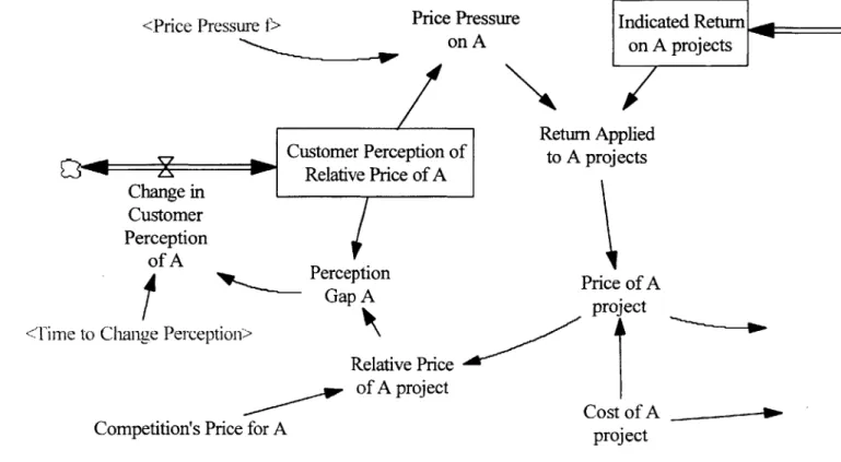
Figure 12: Modified Causal Loop Diagram for "Pressure to Increase Margins" Structure was added to the model which allows ProductCo's price relative to that of the competition to affect the margin which is actually applied when the price is determined. The changes to the model for A projects are shown in Figure Thirteen; only the modified portion is given here. Note that "Return on A projects" has been changed to "Indicated Return on A projects"; this is because now the return

which is indicated by management's desires may not be what is actually applied for pricing due to competitive factors. The same changes were made to the structure which applies to B projects.

<Price Pressure f>

Customer Perc Relative Pri

Price Pressure Indicated Return

on A on A projects Return Applied eption of _{to A projects} e of A <Time tc Change in Customer Perception of A Perception Price of A project Change Perception> Relative Price of A project Cost of A

Competition's Price for A _project

Figure 13: Modified Portion of Model for "Pressure to Increase Margins"

A delay occurs between the relative price changing and the customer perceiving this change. This is due to the fact that customers do not review prices on an instantaneous basis; realistically, they would do this periodically. In this case, a quarterly review is assumed. Other key equations are given below.

Price pressure is applied by adding an effect factor to the margin that is actually used to calculate price: Return Applied to B Projects=Price Pressure on B*Indicated Return on B projects

Units = fraction

Price pressure is a table function with the customer's perceived relative price as an input: Price Pressure on A=Price Pressure f(Customer Perception of Relative Price of A)

Units = dimensionless

Graph Lookup -Price Pressure f

0 I

This table function effectively allows margins to be set at the indicated level if ProductCo's price is below the competition's, while dropping quickly to nearly zero when it is above the competitor's price.

When the model is simulated with the effects of price pressure added, it shows that the desired margin cannot be reached. Figure Fourteen shows this behavior.

Meeting the goal for average return

Average return : price pressure fraction

Desired average return : price pressure -- fraction

Figure 14

After further analysis, it is shown that this is only true if the competitor's price is above ProductCo's cost to execute the project, but below the price that includes the margin that is indicated to reach the desired average margin. As is shown in Figure Fifteen, if the competitor's price is below ProductCo's cost, almost no margin can be charged. This would likely drive ProductCo out of business, or at least away from the projects of this kind. If the competitor's price is high, ProductCo can charge the prices that they need to reach their desired margin, and the goal of 8% is achieved.

0.0799

0.0611

0.0235 0.0047

0

Graph for Average return

--- --- - --- --- - --

---30 60 90 120 150 180 210 240 270 300

Time (Month)

Average return price pressure fraction

Average return high comp price ... faction Average return :low comp price --- fraction

Figure 15

Another fact which is interesting to note is that management's goal continues to rise despite the competitive pressures that are keeping the actual margins down. This is shown in Figure Sixteen.

Indicated Returns

-

Management's Goal

Indicated Return on A projects price pressure fraction Indicated Return on B projects price pressure ---. fraction

Figure 16

What does this mean in the real system? It is likely that management will see what is going on and will not continue to have unrealistic goals. However, it is indicative of the ongoing conflict between desired margin and competitive pressures within the company. ProductCo must then seek ways to relieve this situation.

Given that there is price pressure from the competition that might prevent ProductCo from reaching its goal, what can be done? One avenue to pursue is cost reduction. The next hypothesis proposed addresses this issue.

Hypothesis Two: Cost Cutting Through Resource Reduction

When there is pressure in the system to cut costs, a common response is to reduce resources. This is often done through workforce reductions, either by layoffs or attrition. Hypothesis two maintains that while this reduces costs in the short term, there are often unintended side effects. One potential effect is that the quality of work done is reduced, since the company is trying to do the same amount of work with fewer resources. Figure Seventeen shows the causal loop diagram for Hypothesis Two.

-profits.-+ rework

+

Figure 17: Causal Loop Diagram for "Cost Cutting Through Resource Reduction" Here, the negative loop will tend to drive cost, and by extension resources, to an equilibrium position that can be sustained by profits. However, if this level is not enough to maintain quality work, cost will be driven up by errors. This erodes profitability and can lead to further need for cost reductions. This could lead to a downward spiral if the company is not careful.

As with hypothesis one, a model was created in Vensim; documentation of the full model and all of its equations can be found in Appendix A. Note that this is a new model, not a continuation of the model

built for hypothesis one. The connections and interactions between the two models will be considered later. The first part of the new model, shown in Figure Eighteen, relates to how the pressure to reduce costs can drive the adding and removing of resources.

Bid Cost

Cost Overrun

Actual. Cost _{Pressure to}

reduce costs Cost Due to Engineering Resources Cost due to Materials

Cost per resource _{Effect of Work to}

Effect of Work to Do on Desired Do on Desired Resources f

<WorkToDo> _Resources

Reesource

Relative _{Effect of Pressure}

work to do _{Desired resources-o}

Desired Resource Desired

work to do Resource gap Effect of Pressur

on desired f

PereiedResources

<-numAdding and Initial resource

resources per removing resources

project

Resources _{Time to adjust resources} Perceived ...--- P relative to min

rininm

resources _{<winning projects>}

on

s

s

Figure 18: Model for "Cost Cutting Through Resource Reduction", Part One Following are some of the key equations for this section of the model.

The level of resources is changed by adding or removing resources in response to the gap between the desired and current resource levels:

Resources= INTEG (Adding and removing resources)

Units = people

Adding and removing resources=(Resource gap/Time to adjust resources)

Units = people/Month

Resource gap=Desired resources-Resources

Units = people

The amount of desired resources is calculated using the current resource level with two effects. First is the amount of work to do; this tries to keep the resource level high enough to complete the required tasks. Second is the pressure to reduce costs5_{, which pushes the resource level toward a point which is}

affordable:

Desired resources=Resources*Effect of Pressure on Desired Resources*Effect of Work to Do on Desired Resources

Units = people

The second part of the model shows how work is accomplished. As projects are won, work to do enters the system. These tasks may be performed correctly or incorrectly, which is governed by the quality level. Those that are performed incorrectly are discovered after a period of time, and they re-enter the pile of work to do. The second portion of the model is shown in Figure Nineteen.

s The actual cost includes a component for materials cost. This is not used in this model, but is included to allow for further modeling work on the effects of cost reduction pressure on materials cost.

<Penrces Effect of Resource

Effect of lack of relative to min> Shortage on PDY f <Fractional Correct Work> work on PDY

Normal PDY <Tasks per project> <Actual comi

ime Effect of Resource

zon for Shortage on PDY

yness - Effect of lack o

Work to Do work on PDY CorrectWork

ning projects> required to Accomplishing Tasks Leaving

nig rjets keqed buso Correctly System I

eep

busy Productivity y Maximum Quality

<Resour

17 _Quality

WorkT OD IEffect of Resource

Tasks entering Acconplishin Shortage on Quality

.-system Accomplishing

Incorrectly Undiscovered z

<Resources> Tasksk eA i g

Tasks per sysemv2

project

Discovering

<Tasks per project>

I A:d

pletion rate>

ces relative to min>

Effect of Resource Shortage on Quality f

Actual completion rate>

-rcdLton1a U11Kuvulu r1WV

Time to discover rework

Figure 19: Model for "Cost Cutting Through Resource Reduction", Part Two

T Hori bus

<win

The equations in this section revolve around the rate at which work gets done, and how much of it is done correctly6. The key equations are given below.

The rate at which work gets done is controlled by the resources that are available and their productivity: AccomplishingWork= Resources*Productivity

Units = tasks/Month

Productivity can change from its normal level for two reasons. It can increase slightly when there begins to be a resource shortage, since people are forced to take on more work. It can also decrease if there

is not enough work available to be done:

Productivity=Normal PDY*Effect of lack of work on PDY*Effect of Resource Shortage on PDY

Units = tasks/(Month*person)

The quality level dictates how much work is done correctly, and how much is done incorrectly:

AccomplishingCorrectly = AccomplishingWork * Quality

AccomplishingIncorrectly = AccomplishingWork * (1 - Quality)

Units = tasks/Month

Quality is influenced by the amount of resources that are available, relative to a minimum level that is needed to work effectively:

Quality=Normal Quality*Effect of Resource Shortage on Quality

Units = fraction

Work leaves the system when a project is complete. Since the participants in the system do not know which work has been completed correctly until rework is "discovered", tasks can leave the system both

from Correct Work and Undiscovered Rework. The total rate of projects being completed is

6 _{This section of the model is based on the "work accomplishment structure", also called the "rework cycle". It is}

found in many well known project models. This author used as references the molecules in Vensim (a set of commonly found modeling structures) and the teachings of Dr. James Lyneis in the fall 1998 session of the System and Project Management course at MIT.

controlled by the next section of the model. This completion rate is then divided proportionately and converted to units of tasks. For example, the equation for tasks leaving Correct Work, called Tasks Leaving System 1, is:

Tasks Leaving System 1 =Actual completion rate*Fractional Correct Work*Tasks per project

Units = tasks/Month

The third portion of the model, which as noted above controls the completion of projects, is shown in Figure Twenty.

Initial Active Projects

winning pro

jects

Desired Completion Rate Average time to complete project completing projects Actual completion rate Effe Relative rework discovery

ct of rework discovery

on completion

<DiscoveringRework>

<Tasks entering system,

Effect of rework discovery

on completion f

Figure 20: Model for "Cost Cutting Through Resource Reduction", Part Three The desired rate of completion is dictated by the average time to complete a project:

Desired Completion Rate=Active Projects/Average time to complete project

The actual rate of completion may be reduced if the company feels that the quality of work is slipping. This is judged based on the proportion of work coming in that is rework. If rework being discovered is more than 25% of the total tasks entering Work To Do, ProductCo reduces the rate at which projects are allowed to leave the system.

Actual completion rate=Desired Completion Rate*Effect of rework discovery on completion

Units = projects/Month

Relative rework discovery=DiscoveringRework/(DiscoveringRework+Tasks entering system)

Units = fraction

The behavior of this model is much more difficult to predict than that of hypothesis one. We have two competing pressures -pressure to reduce cost, and pressure to get the work done. It is possible that one of these will be dominant and overcome the other. That is, the pressure to reduce costs could be so powerful that all other considerations are lost. Alternatively, one factor could dominate up to a point, to be superseded by the other when a certain level is reached. This is a strength of system dynamics

-to show behavior which is not intuitively obvious due -to the complexity of the system.

When initially run, the model quickly reaches equilibrium. Figure Twenty-One shows the behavior of the resource level. It drops to a point which balances the effects of the cost overrun and the need to get work done. The effects are shown in Figure Twenty-Two.

Graph for Resources

--- - --- ---- - -- ---- - -m-

--0 20 40 60 80 100 120 140 160 180 200

Time (Month)

Resources : base people

Figure 21

Effect of Price Pressure and Effect of Work To Do

20 40 60 80 100 120 140 160 180 200

Time (Month)

Effect of Pressure on Desired Resources : base dmnl

Effect of Work to Do on Desired Resources : base -.-.-.---- dmnl Figure 22 500 465.21 430.42 395.63 360.84 1.738 1.344 0.9512 0.5577 0.1643 0

-

-.

--

..-

-~..--.~ ~-.- -~.-

--..-

~ -- - - -

---~~

- - -- - -

---

- - - --.-.-.--..-

-==....

-...

--...

~--. -...

---....

-...

--.

~...

-...

~

~

~....

-...

...

...

~...

This stabilizes the cost overrun, although it does not eliminate it. The graph for Cost Overrun is given in Figure Twenty-Three. Because, as shown above, there is continuing pressure to keep resources at a level that is adequate to keep Work to Do from piling up, the cost overrun does not reach zero in this scenario.

Graph for Cost Overrun

5,000 3,956 2,912 1,868 825.24 0 20 40 60 80 100 120 Time (Month) 140 160 180

Cost Overrun : base

200

dollars

Figure 23

This points out an issue that ProductCo must address. They will need to find ways to reduce costs other than reducing resources. Alternatively, they can try to find ways to get more out of the resources that they have. This will be discussed in more detail later in this section.

-As pointed out, keeping resources at a certain level allows work to move smoothly through the system. Work to Do is shown in Figure Twenty-Four. It initially grows as resources are cut, then levels off as resources stabilize.

Graph for WorkToDo

20 40 60 80 100 120

Time (Month)

140 160 180

WorkToDo : base tasks

Figure 24

One surprising aspect of the Work to Do graph is that it decreases after it reaches its peak. This occurs because the rate of accomplishing work remains above the total inflow (Tasks Entering System plus Discovering Rework) until the equilibrium resource level is reached. This tells us that in the real system,

if the backlog of Work to Do is to be reduced, then the rate of work getting done must be greater than the work coming in. This is fairly obvious; however, what might not be obvious is that we have to

consider the flow of rework being discovered as well as the new work entering the system. 116,734 112,863 108,992 105,121 101,250 0 200

Further analysis was performed on the model by placing it in equilibrium, then exciting it by adding an input that pushes it out of its equilibrium state. The response to this change can yield some insights into the behavior of the real world system. In this case, the rate of projects was stepped up by one per month. The added model structure is shown in Figure Twenty-Five. When the switch is turned "on" by setting its value to one (normal value is zero), it activates a step function which increments the rate of winning projects by one, starting at time 500.

step in projects

switch for step

Active

winning projects Projects completing projects

Figure 25

This change creates an increase in the work to be done. This, in turn, increases the required resources. The behavior of the stock of Resources is shown in Figure Twenty-Six. It rises to a new, higher equilibrium. The interesting aspect is that it does not rise at a steady rate. Note that the Resources curve is exactly the same shape as the Cost Overrun curve, since the cost in this model is controlled only by resources.

Graph for Resources

This change in slope is a result of the effects that are impacting the Desired Resources. One possibility is that one effect is dominating, but is then overcome by the other. However, this is not the case; if it were, a change in the direction of the resource curve would be likely since the effects are pulling in opposite directions. Figure Twenty-Seven shows the resource curve overlaid with the effects. Another possibility is that the changing slopes of one of the effects is causing the discontinuity in the Resources

curve. 500 465.20 430.41 395.62 360.83 0

Resource Level vs. Effect of Price Pressure and Effect of Work To Do

Effect of Pressure on Desired Resources : equil dmnl

Effect of Work to Do on Desired Resources : equil ... dmnl Resources: equil --- people

Figure 27

Both of the effects are calculated using table functions. These are shown in Figure Twenty-Eight, with the table function for Effect of Work to Do on Desired Resources on the left, and the table function for Effect of Pressure on Desired Resources on the right.

-.. . .

. . . . .. . . . . .. .. ... . . . . .. . . .. . . . . .. . . .

Graph Lookup -Effect of Work to Do on Desired Resources f Graph Lookup -Effect of Pressure on desired f 20

0 0

0

-Figure 28: Table Functions

In order to determine whether the changing slope of one of these functions was causing the shape of the Resources curve, simulations were run which removed points from each table function, rendering them more linear. Points were removed between x = 0.5 and 1.0 in the case of the effect of work to do. The results of these simulations are shown in Figure Twenty-Nine. The table for Effect of Pressure on Desired Resources was reset to its original shape, and points were then removed between x = 0 and 1.0 in the table function for the effect of pressure. The results of these simulations are shown in Figure Thirty.

500 465.20 430.41 395.62 360.83 0 Resources Resources Resources 510.62 466.88 423.14 379.41 335.67 0

Graph for Resources

--- - --- -- -- I ...- 150 300 450 Time 600 (Month) 750 900 equil :chg w ork to do I ... - - -.-.. -. - - - - -. - - -. : chg work to do 2 ---Figure 29

Graph for Resources

~-~~- ~- -~- -~~ -- ~ ~ -- - - -- - - -- - -1I 150 300 450 Time people people people 600 (Month) 750 900 equil chg pressure 1 chg pressure 2 people .--- -- people - -- - - -- -- - - - -- - - - - p eop le Figure 30 Resources Resources Resources

Changing the shape of the table function for the Effect of Work to Do on Desired Resources does not change the shape of the Resources curve. It only shifts it slightly, reaching equilibrium sooner. This is because as the table function is made more linear, it causes the system to react faster to the buildup of work to do. It pulls the resources up more quickly in response, and it reaches a higher equilibrium level of resources since the counteracting effect due to price pressure has not changed.

On the other hand, changing the shape of the table function for the Effect of Pressure on Desired Resources has a more dramatic effect on the shape of the Resources curve. It first removes the step in the curve, and then causes an overshoot and recovery pattern. When the table function is completely

linear between x = 0 and 1.0, the resource level overshoots and then oscillates briefly before reaching its equilibrium level, which is higher than the original equilibrium level. This occurs because removing the points from the table function causes the system to react more slowly to the rising cost overrun. It

allows resources to build in response to the work to do, and then works to bring them down when the cost overrun gets too high.

This analysis points out that if the company does not react strongly enough to cost overruns, the eventual problem will be worse. In the original setup, the Effect of Pressure on Desired Resources, which is a multiplier on Desired Resources, dropped off quickly as the Actual Cost moved above the Bid Cost. The fact that the exact points used in the table function caused a step in the curve for Resources is less important; a smoother table function could eliminate this issue. The biggest insight for ProductCo is that they must respond quickly to cost overruns if they want to keep the equilibrium level of cost to a

There is another issue to be considered, however. If ProductCo reacts too harshly to cost overruns, they may damage their quality. The table function can be changed by shifting points, rather than by eliminating them, to show a quicker response and a slower response to cost issues. The resulting Resources curve is shown in Figure Thirty-One.

Graph for Resources

500 461.21 422.43 383.65 344.87 0 150 300 450 600 750 900 Time (Month)

Resources: equil people

Resources : quick cost resp ... people Resources : slow cost resp --- people

Figure 31

Responding quickly to cost keeps the cost overrun lower, while responding more slowly allows it to become higher. It would seem that ProductCo should follow the policy which produces the lowest cost overrun. But this creates other problems; the graph for quality is shown in Figure Thirty-Two. Since there is an effect on quality which is strongly correlated to the resource level, the quality is also at its lowest point when the company responds harshly to cost overruns.

-- - - -- - - -- - - -- --- -- - ----

-....

...

...

...

...

...

. _

....

-.

.

.

..

..

.

..

..

.

.

.

.

_

Graph for Quality

Quality :equil fraction

Quality quick cost resp ... fraction Quality slow cost resp --- fraction

Figure 32

Note that quality takes an initial hit at time 500 because although work has been added, resources cannot be added instantaneously. However, in the original formulation or with a slow cost response, it recovers to approximately its previous level. With a quick cost response, resources remain short and

quality does not recover.

One could predict that this would lead to excessive work to do, since the rework would be increased if the quality is lower. The work to do pile does reach a higher level when the cost response is faster, but it is not due to rework. Figure Thirty-Three shows the graph for Work to Do, while Figure Thirty-Four shows the rate of Discovering Rework.

Graph for WorkToDo

WorkToDo quick cost resp ... WorkToDo slow cost resp

---Figure 33

Graph for DiscoveringRework

tasks tasks tasks 150 300 450 600 Time (Month) DiscoveringRework: equil

DiscoveringRework : quick cost resp -- ---. DiscoveringRework : slow cost resp

---tasks/Month tasks/Month tasks/Month Figure 34 22,500 17,110 11,721 6,332 943.18 0 750 900

- - - -

- - -- - -

-

-....

- -

-...

---This shows that with the slower cost response, the rate of rework discovery does not change

significantly, and it actually drops slightly with the quicker response. How is this possible? As it turns out, with the quicker cost response, the work is flowing more quickly into Undiscovered Rework, but it is being shipped out the door before it is discovered.

Comparing the quick cost response case to the original equilibrium case, we can see why this occurs. If the quality does not recover fairly quickly, the proportion of work that is flowing into rework remains high. This raises Fractional Undiscovered Rework, which compares the level of undiscovered rework to the total work perceived to be complete (Correct Work plus Undiscovered Rework). The graph for Fractional Undiscovered Rework is shown in Figure Thirty-Five.

Graph for Fractional Undiscovered Rework

0.3591 0.2736 0.1882 0.1027 0.0173 S- --- .--- --- ---0 150 300 450 600 750 900 Time (Month)

Fractional Undiscovered Rework: equil fraction

Fractional Undiscovered Rework: quick cost resp ... fraction Fractional Undiscovered Rework: slow cost resp --- fraction

The large jump in Fractional Undiscovered Rework occurs at the same time that the overall completion rate increases. When the incremental project was added, the desired completion rate for projects

increased. Projects are expected to be completed at the same rate despite the fact that resources cannot be added instantaneously. These two factors cause an increase in the rate of tasks flowing out of Undiscovered Rework, called Tasks Leaving System 2. This is shown in Figure Thirty-Six.

Graph for Tasks Leaving System 2

2,775 2,104 1,432 761.23 89.82 - -.- -- --- ---- --- --- --- T --0 150 300 450 600 750 900 Time (Month)

Tasks Leaving System 2: equil tasks/Month

Tasks Leaving System 2 : quick cost resp ... tasks/Month Tasks Leaving System 2 : slow cost resp --- tasks/Month

Figure 36

Since Undiscovered Rework begins leaving the system faster at about the same time that it starts being created faster, the net impact on the level of Undiscovered Rework is a minimal change. The impact on ProductCo could be much greater. With the quick cost response, they are shipping projects with many more errors. This low quality level will not be well received by their customers. This would likely result

in a lower rate of winning projects over time. This can be addressed when hypotheses one and two are combined.

If it is not due to rework, the buildup in Work to Do must be attributable to some other factor, namely the rate of accomplishing work. Because the quicker cost response limits the amount of rework that

can be added, it also limits the amount of work that can be completed in a given time period. Productivity actually increases slightly with the quicker cost response. People can increase their productivity in response to a resource shortage, but only to a certain point. And, as noted previously, quality of that work will suffer. The graph for Productivity is shown in Figure Thirty-Seven.

Graph for Productivity

Productivity equil tasks/(Month*person)

Productivity quick cost resp ---..--.-- tasks/(Month*person) Productivity slow cost resp --- tasks/(Month*person)

Figure 37

---However, this cannot make up for the lack of resources. The graph for Accomplishing Work is given in Figure Thirty-Eight. Since work cannot flow out of Work to Do as quickly, the backlog builds up to a higher level, as was seen in Figure Thirty-Three.

Graph for AccomplishingWork

AccomplishingWork: equil tasks/Month

AccomplishingWork : quick cost resp ... tasks/Month AccomplishingWork : slow cost resp --- tasks/Month

Figure 38

This buildup of work to do does not affect the rate at which projects are being shipped out the door in this model, although with the quick cost response they are being shipped with many more errors.

However, it may make it more difficult to get a high-priority project pushed through the system quickly, since work is accomplished fairly slowly and there are many tasks waiting to be addressed.

The equilibrium analysis of this model yielded several insights for ProductCo. The response of the company to a cost overrun is vital. A strong response can ensure that the cost overrun is limited.

- - --- - -- ---- - - - ---- ---- -- -- ---

-...

However, this has serious repercussions on quality. The analysis also shows that this quality problem may be hidden by the fact that the errors are being shipped out before they are discovered. If

ProductCo uses relative rework discovery as an indicator of when it is okay to ship, this problem could begin to effect customer perceptions before ProductCo is even aware of it. Finally, with limited resources, work cannot move through the system quickly, which could cause issues if a high-priority project must be expedited.

Using the model, I also looked at which factors have the biggest impact on the dynamics of the system when they are changed. The model is very sensitive to the values used for Cost per Resource and for Normal Productivity. This makes sense, as both of these parameters directly affect how much work we can get for every dollar we spend on resources.

By varying the Cost per Resource from its base value of 30 to a lower level of 25 and a higher level of 35, we can see how this affects the dynamics of the model. The graph for Resources is shown in Figure Thirty-Nine. As expected, a higher cost leads to a lower resource level, but the shapes of the curves are not the same.