Towards a generic power estimator

Open Archive TOULOUSE Archive Ouverte (OATAO)

OATAO is an open access repository that collects the work of Toulouse researchers and

makes it freely available over the web where possible.

This is an author-deposited version published in :

http://oatao.univ-toulouse.fr/

Eprints ID : 13199

To link to this article :

DOI :10.1007/s00450-014-0264-x

URL :

http://dx.doi.org/10.1007/s00450-014-0264-x

To cite this version :

Fontoura Cupertino, Leandro and Da Costa, Georges and

Pierson, Jean-Marc Towards a generic power estimator. (2014) Computer

Science - Research and Development, en ligne. pp. 1-9. ISSN 1865-2034

Any correspondance concerning this service should be sent to the repository

administrator:

[email protected]

Towards a generic power estimator

Leandro Fontoura Cupertino · Georges Da Costa · Jean-Marc Pierson

Abstract Data centers play an important role on world-wide electrical energy consumption. Understanding their power dissipation is a key aspect to achieve energy efficiency. Some application specific models were proposed, while other generic ones lack accuracy. The contributions of this paper are threefold. First we expose the importance of modelling alternating to direct current conversion losses. Second, a weakness of CPU proportional models is evidenced. Finally, a methodology to estimate the power consumed by applica-tions with machine learning techniques is proposed. Since the results of such techniques are deeply data dependent, a study on devices’ power profiles was executed to generate a small set of synthetic benchmarks able to emulate generic applica-tions’ behaviour. Our approach is then compared with two other models, showing that the percentage error of energy estimation of an application can be less than 1 %.

Keywords Power estimation · Generic model · Data centers · Machine learning · Neural networks

1 Introduction

The number and size of data centers is continuously increas-ing durincreas-ing the last years. The popularity of data centers turned them into one of the most power demanding facilities. The

L. F. Cupertino (

B

e-mail: [email protected] G. Da Costa

e-mail: [email protected] J.-M. Pierson e-mail: [email protected]

use of data centers is divided into high performance com-puting (HPC) and Internet services, or Clouds. Performance is crucial in HPC environments, while on Cloud systems it may vary according to their service-level agreements. Some data centers even propose hybrid environments. All of them are energy hungry, modelling their dissipated power is the first step to achieve better monitoring, management, usage policies and energy savings.

Energy efficiency can be enhanced either by hardware replacement, where newer hardware will provide a better performance, or by understanding their software usage. Pre-vious works in power modelling of computing systems pro-posed the use of system information to monitor the power consumption of applications, but these models are either too specific for a given kind of application or not accurate enough.

This paper proposes a methodology to create a unified power model based on standalone and parallel systems. The contributions of this paper are threefold. First we show the importance of using direct current power measurements to generate a model, an aspect that has been neglected by some

authors [5,11]. Second a study on the limits of CPU

propor-tional models is done. Finally, we propose a methodology to achieve generic models capable of addressing any kind of applications and compare it with existing models.

This paper is organized as follows. Section2provides a

summary of the state of the art on computing system’s power modelling. Some techniques to accurately measure power

are described in Sect.3. Section4states the power

estima-tion technique and the limitaestima-tion of current CPU proporestima-tional

models. Section5presents the results of the alternating (AC)

to direct current (DC) conversion power modelling, a com-plete power profiling, along with the training, validation and limits of the proposed methodology. Conclusions are given

2 Related work

The most common approach to model system’s power con-sumption is to use CPU capacitive models. These models

have a general formula P ∼ u(cv2f )to estimate the power

based on the processor’s frequency f , voltage v, usage u and effective capacitance c. A linear combination of capac-itive model of processor’s device for multi-core processors

including power saving techniques was proposed in [1]. The

model is validated using two synthetic benchmarks with reported errors under 9 % (3W). Although the results show an acceptable error, the use of synthetic benchmarks for model validation may not be significant in real world appli-cations. The drawback of such model is that one need to have precise information regarding the capacitance of eight processor’s components and processor’s frequency/voltage table.

Another common technique is to use performance coun-ters to automatically extract a model. Several linear regres-sion power models for HPC applications were proposed

in [9]. The choice of which models to use is done at runtime

based on a decision tree. The models’ variables are selected from a set of performance counters and CPU temperature sensors which present the highest correlation with system’s power. The reported error is of 5 % maximum.

The use of hardware specific sensors were explored in

[13]. The authors extended Performance API (PAPI) to

direct measure power consumption of Intel’s CPU via Run-ning Average Power Limit (RAPL), and Nvidia’s GPU via NVML. This approach does not try to model the power but can be a good way to evaluate the power of HPC applica-tions, gathering the dissipated power instead of modelling it with system’s variables. The results should be more pre-cise than using models, although this comparison was not made.

The methodology to create power estimators presented in this paper differ from the above mentioned works as follows: (a) it provides a nonlinear model that takes into account not only the CPU, but the entire system; (b) it proposes a generic set of synthetic benchmark to model not only HPC appli-cations but any application; and more importantly, (c) it is not hardware dependent and does not require architecture information of the hardware.

3 Power metering

Power measurement is a key feature to understand power consumption of systems and devices. A common technique is to use a digital multimeter to measure the voltage drop across a shunt resistor and to compute the power dissipated on the wire. This technique monitors power usage on each Power Supply Unit’s (PSU) power rails, providing a detailed

usage of system’s power [2]. However, the inclusion of a

resistor between the power rails may not be feasible in some architectures.

Some vendors provide integrated monitoring solutions on their hardware. For instance, Dell’s PowerEdge M1000e enables real-time reporting for enclosure and blade power consumption. Intel introduced a model specific register, namely RAPL, to provide power and energy measurements at different processor levels. RAPL is only available in recent

architectures [8].

Even though the above mentioned techniques measure power in DC circuits, the most architecture independent and less intrusive method is to measure AC power at the outlet. General purpose solutions are widely available on the

mar-ket, like Plogg, Kill-A-Watt1and Watts Up?.2 In addition,

AC power is used by energy providers to charge their clients. Therefore, if the economical aspect of energy efficiency in a data center will be evaluated, AC power needs to be esti-mated. The disadvantage of this technique is that it can only measure system-level power.

4 Power estimation

The estimation of power consumption of a system is based on workload observations. The system is stressed into differ-ent conditions, while a set of predefined Key Performance Indicators (KPIs) along with its power consumption are

pro-filed [10]. To avoid modelling noise, it is important to

decou-ple the static from the dynamic power consumption.

4.1 Dynamic power decoupling

Dynamic power is the fraction of the dissipated power which varies according to hardware usage. Most authors consider the dynamic power as being the difference between the total and idle power consumption.

However, when using an AC power meter, one should consider the energy conversion losses as well. Although the power suppliers usually provide an average efficiency rate,

like the 80 Plus label,3 their efficiencies are not constant,

which implies that their AC to DC conversion losses need to be modelled. Our experiments show that the power con-version losses can vary from 26 to 380 W per blade, which will have a significant impact when using AC power data to generate power models. More detailed results will be shown

in Sect.5.

1 _{Seehttp://www.p3international.com.} 2 _{Seehttp://www.wattsupmeters.com.} 3 _{Seehttp://www.80plus.org.}

0 1 2 3 4 35 40 45 50 55 60

Number of stressed cores

A ver age P o w er (W), σ <0.85 ALU CU FPU Rand

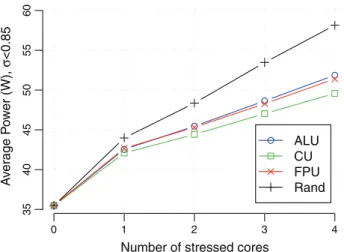
Fig. 1 Average power dissipated by an Intel Core i7-3615QE

Proces-sor with four physical cores, when running different benchmarks at different CPU loads

4.2 Limitations of CPU proportional models

The use of CPU proportional models to estimate proces-sor’s power consumption is extensively done in the literature. These models are based on the CPU’s percentage usage. The accuracy of such models was evaluated by running four micro benchmarks (µ-benchs) to analyse the impact of each proces-sor’s main components: control unity (CU), arithmetic logic unit (ALU) and floating-point unit (FPU). Given the impact of the random number generation, a fourth benchmark was developed to exploit it (Rand). Each µ-bench was executed increasing the number of active cores of the system while keeping their frequencies constant at 2.3 GHz in an Intel Core i7-3615QE processor.

Figure1summarizes the results, where each data point

is the average of 1,000 power measurements. The results show that, as the number of active cores increases, the power dissipated by the processor’s package increases in a different rate, i.e. in a multicore processor, power dissipation is not linear to core’s usage. Furthermore, the power dissipated at the same CPU load vary according to application’s behaviour. This variation can reach up to 7 W when all four cores are stressed, implying that the use of CPU proportional models can provide an error of up to 15 % depending on the training set used for calibration.

4.3 Key performance indicators

Performance indicators can be divided into two classes: hard-ware and softhard-ware sensors. Hardhard-ware sensors are strictly related to system’s architecture and their availability and implementation may change according to vendors. Some common hardware sensors are CPU’s thermometer and per-formance counters. The first measures the temperature, while

the latter contains a set of event counters to monitor different aspects of an application, such as the number of cache misses and cycles. Software sensors depend mainly on the operating system’s capabilities. They can provide information such as processor’s phase (P-states) and idle states (C-states), net-work traffic and memory usage.

The inputs of an estimator need to be carefully selected. Usually their selection is done based on a priori knowledge. As we want to address any architecture and we do not know which KPIs will be available the target hardware, we used the biggest quantity of variables we could, providing a high num-ber of degrees of freedom to create the estimator discussed later on.

The monitored performance indicators were measured through system information (SYS), performance counters (PC) and model specific registers (MSR). Typically on Unix-like systems, system information sensors come from the

/procand /sys file systems. Performance counters were

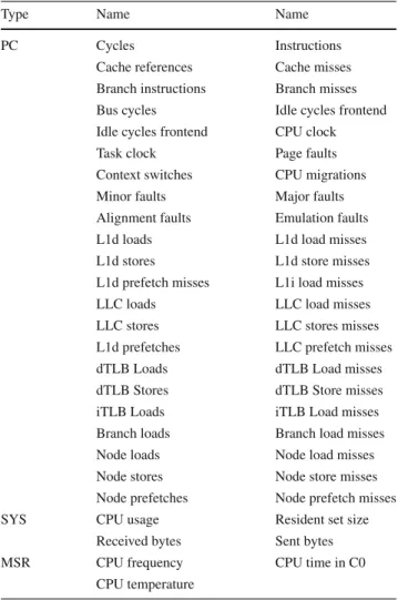
collected using Linux perf tool. MSR registers provide information of core’s frequency, temperature and time in active state (C0). The complete list of explored variables

can be found in Table 1. Data acquisition was done using

ectoolsand extending its library [3] to include all listed

KPIs.

4.4 Machine learning

Machine learning is a field of Computer Science which intends to automatically extract knowledge from a set of observed data. This section describes how the training set (TS) must be created as well as two machine learning tech-niques used in this paper: Linear Regression and Artificial Neural Networks.

The training set is a matrix, where each row contains one observation of the system, including inputs and targets. When modelling the power consumption of a system, each row of in the TS is a historical entry. The training set can be decom-posed into a matrix X of KPIs and a target vector y of power measurements. The accuracy and range of both are of great importance when creating precise models, i.e. the data must contain valid information and should enclose the entire range of usage for each variable. A set of synthetic benchmarks designed to stress specific devices of a system over time is commonly used to generate a TS on any hardware.

Linear Regression (LR) is a statistical tool widely used to define the parameters’ weights of a predefined function. In the hardware power modelling perspective, it can be used to calibrate existing models for usage in new hardware. This technique is fast to be computed and provides adaptability for existing models, however is not quite adequate to cre-ate new ones since it does not handle nonlinear relationship between the variables. A common technique is to linearize some variables to calibrate nonlinear models.

Table 1 Monitored KPIs

Type Name Name

PC Cycles Instructions

Cache references Cache misses Branch instructions Branch misses Bus cycles Idle cycles frontend Idle cycles frontend CPU clock Task clock Page faults Context switches CPU migrations Minor faults Major faults Alignment faults Emulation faults L1d loads L1d load misses L1d stores L1d store misses L1d prefetch misses L1i load misses LLC loads LLC load misses LLC stores LLC stores misses L1d prefetches LLC prefetch misses dTLB Loads dTLB Load misses dTLB Stores dTLB Store misses iTLB Loads iTLB Load misses Branch loads Branch load misses Node loads Node load misses Node stores Node store misses Node prefetches Node prefetch misses

SYS CPU usage Resident set size

Received bytes Sent bytes MSR CPU frequency CPU time in C0

CPU temperature

Artificial Neural Networks (ANN) is a branch of Compu-tational Intelligence that mimics the behaviour of biological neurons. It has been used in problems of series prediction,

pattern recognition and function approximation [6]. ANN can

be used as a non-linear mathematical model to find complex relationships between inputs and targets of an unknown func-tion. It also has a concept of weight matrices which provides the parameterization of the model, although the quantity of weights is larger than those used in LR. For regression prob-lems a specific class of ANN, called multilayer perceptron (MLP), is used. MLP is a feedforward ANN composed of one or more hidden layers. Each layer computes its output as follows:

a = ϕ(Wi + b) (1)

where W is the weight matrix, i is the input vector of the cur-rent layer, b is the bias vector, ϕ(·) is the activation function and a is the output vector. This means that in the input layer,

i is the row vector xi ∈ X; while for the final layer a is the

model’s estimation ˆy.

The learning of a MLP is done based on a backpropaga-tion algorithm, which uses partial derivatives of the estimate error to adjust W and b. This algorithm requires the acti-vation function to be differentiable. It has been proved that two-hidden-layer feedforward networks can learn any dis-tinct samples with any arbitrarily small error using a sigmoid

activation function [7].

4.5 Accuracy evaluation

The evaluation of the quality of our proposed methodology and consecutive results will be compared with two models. As a reference value a constant model, representing the aver-age power consumption of the TS will be used as a naive implementation. The second is a capacitive model, the most used model for DVFS systems. This model will consider that the voltage is constant and can be approximated by

w0+ w1∗ %cpu ∗ f r eq. The weight calibration is done

through a linear regression of the training set. These models will be further referred as const and capac, respectively. Models’ comparison is realized based on the correlation

(R2) between estimated and measured values, as well as two

error metrics, mean absolute percentage error (MAPE) and energy percentage error (EPE), defined as follows:

MAPE = 100 N × N ! i =1 " " " " yi− ˆyi yi " " " " ; (2) EPE = 100 × " " " " " #N i =1yi−#i =N1ˆyi #N i =1yi " " " " " , (3)

where y is the measured power (target), ˆy is the estimated value and N is the total number of samples.

5 Experimental results

In this section we describe the environment setup, the power decoupling methodology, the hardware and training set pro-filing. Later, we present the power estimation results and limitations.

5.1 Environment setup

The experiments were run on a RECS compute box [12].

The RECS compute box is a high density server prototype composed by 18 modules connected through a backplane controller. Each module operates as an independent com-puter composed by a processor, memory, network and fan. In the experiments we exploited a module with Intel Core i7-3615QE processor, 16 GB of RAM and Intel 82579LM Giga-bit Ethernet. All nodes (modules) are diskless and boot the same OS image (Scientific Linux release 6.4; kernel v2.6.32).

0 200 400 600 800 1000 1200 1400 0 200 400 600 800 1000 AC Power (W) DC P o w er (W) Measured Modeled

Fig. 2 PSU’s AC to DC power conversion modelling

A Plogg power meter, with a sampling rate of 3 Hz and a precision of 1 mW, were included to monitor the power dis-sipated by the PSU.

The modules management and power monitoring is done by a external server to not impact the measurements. For similar reasons, KPIs and power synchronization was done offline.

5.2 Power decoupling

Power decoupling is a methodology to reduce noise at the power measurements. The vendor of our test bed’d PSU made available a set of data points with PSU’s input and output

power [12]. These data were used to model the PSU’s

alter-nate (PAC) to direct (PDC) power conversion. The model was

done through a linear regression of the following equation:

PDC = w0+ w1PAC + w2P_AC3 , where w0, w1and w2are

constants set to −30.00, 0.8611 and −6.55 ∗ 10−8,

respec-tively. Figure2plots measured and modelled data, the

corre-lation between them is 0.9999, which represents a very good approximation. The remainder of the infrastructure power (fans, driver controller) is considered to be constant and its modelling is embedded into the estimators’ constants.

5.3 Hardware profiling

Hardware profiling requires the development of synthetic benchmarks to measure the impact of each system’s device on the total power consumption. Each benchmark was executed for 1,000 s with a power sampling rate of 1 Hz. These large samples enable us to estimate the confidence interval of the measurements based on the central limit theorem to insure

that our results are statistically acceptable [14]. The analysis

of hardware profiles enables the generation of a small set of synthetic benchmarks to reproduce several devices’ behav-iour. This set of benchmarks will later be used to collect TS data for our machine learning models.

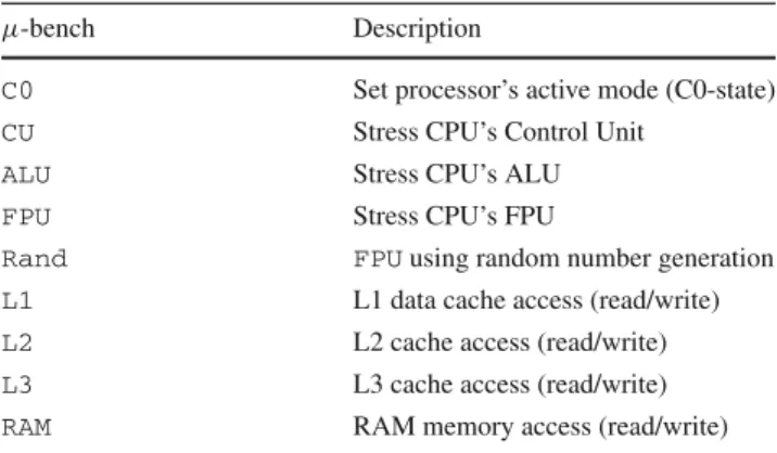
Table 2 Summary of micro benchmarks used for hardware profiling

and training set generation

µ-bench Description

C0 Set processor’s active mode (C0-state)

CU Stress CPU’s Control Unit

ALU Stress CPU’s ALU

FPU Stress CPU’s FPU

Rand FPUusing random number generation L1 L1 data cache access (read/write) L2 L2 cache access (read/write) L3 L3 cache access (read/write) RAM RAM memory access (read/write)

5.3.1 Micro benchmarks

Micro benchmarks (µ-benchs) are synthetic benchmarks

designed to stress specific system’s devices. Table2describes

nine µ-benchs designed to analyse different hardware’s components. All µ-benchs are single threaded, allowing

cpulimitand taskset to define their processor’s core

maximum load and affinity, respectively. The µ-benchs impact over the machine’s power consumption is discussed in the following sections. Micro benchmarks’ source codes

are available online.4

5.3.2 Processor

The processor is claimed to be the most power consuming

device in the system. Figure1summarized the impact of each

processor’s component on the overall power consumption while fully stressing each core. One can notice that the power of ALU and FPU are quite close for all stressed levels.

Cache usage was evaluated by running the same code but accessing different memory positions to force cache misses. Synthetic benchmarks L1, L2, L3 and RAM guaran-tee memory read/write accesses to their respective memory, i.e. L1 makes only L1-data cache accesses, L2 only L2 cache accesses and so on. Processor’s frequency was set to

oper-ate at 2.3 GHz. In Fig.3, one can notice that the memory

access pattern will impact, not only on the execution time of an application, but also its power consumption, having a substantial influence on the overall energy consumed by an application. The difference between the L1d and RAM memory is ≈2.55 W.

Dynamic Voltage and Frequency Scaling (DVFS) was evaluated by running Rand benchmark in four cores and modifying the operating frequency to all available frequen-cies from 1.2 to 2.3 GHz and using Intel Boost Technology,

L1d L2 L3 RAM 43 44 45 46 A ver age P o w er (W) Read Write

Fig. 3 Power profile of data access in several memory levels

1.0 1.5 2.0 2.5 3.0 3.5 30 40 50 60 70 Processor's frequency (GHz) A ver age P o w er (W) Loaded Idle (C0) Idle (CX)

Fig. 4 DVFS impact during the execution of Rand µ-bench

which may operate at up to 3.3 and 3.1 GHz when stress-ing one and four cores respectively. The impact of usstress-ing the Boost technology is very important and can represent a dif-ference of 26 W when compared to the minimum allowed

frequency (Fig.4).

Finally the impact of deepest idle state (CX) power savings are measured by forcing the system to have no latency (C0) when idle and comparing it with the system idle on CX for all frequencies. The results show that the power in CX is barely the same for all frequencies (≈35.47 W). In addition, by comparing the idle power dissipated in C0 and CX, one can see that power savings due to the idle states can reach from 9.62 to 16.51 W depending on its frequency. This evidences the importance of using the time spent in idle states as a variable when tackling a general power model.

5.3.3 Random access memory

The impact of size of the allocated memory on power con-sumption was evaluated by gradually increasing the size of the total allocated resident memory from 1 to 14 Gb. The memory allocation was tested with three cases: read, write and idle. All these cases kept one core of the system busy.

The results of Fig.5show that the average power is barely

the same as when the system has one core fully stressed

(≈43 W, see Fig.1) for all memory accesses and resident

memory size, i.e. the amount of allocated RAM memory do

2 4 6 8 10 12 14 42.0 42.5 43.0 43.5 44.0 Allocated memory (Gb) P o w er (W) Read Write Idle

Fig. 5 Memory allocation impact on system’s power

0 200 400 600 800 36 37 38 39 40 41

Network throughput (Mbits/s)

P o w er (W) Download Upload

Fig. 6 Network usage impact on the overall power consumption for

an Intel 82579LM Gigabit Ethernet

not impact the system’s power consumption. However new

technologies intend to switch memory ranks on and off [4],

generating a new demand for power modelling.

5.3.4 Network interface card

The Network Interface Card (NIC) was evaluated executing the iperf3 tool, which enables the user to stress the network under predefined bandwidth. This way, we started a server at the front-end side and a client at the module and stressed

the network in a 10 % increasing steps scenario. Figure6

shows that the network usage can impact the total power consumption of up to 6 W, i.e. the difference between fully loaded (41.5 W) and idle (35.5 W) system. Its important to notice that an evaluation of NIC’s power from an outlet meter, will measure not only the NIC but also processor and memory consumption. When running these setups, we observed that the CPU usage was always below 5 %, thus its influence on these experiments was neglected.

5.4 Training set profiling

The training set (TS) is a crucial aspect of supervised machine learning. Based on the analysis of the hardware power

execution of these configurations, system’s KPIs (Table1) and power are logged.

The synthetic benchmarks were set up to profile the three main devices (processor, memory and NIC) independently and the maximum (peak) power consumption. Disk IO is not taken into account because we exploit a diskless environ-ment. All µ-benchs were executed in three CPU frequencies: minimum (1.2 GHz), maximum user defined (2.3 GHz) and Boost enabled (up to 3.3 GHz). They also have the same duration per configuration (10 s).

The processor profile was executed to extract most infor-mation from it. Device’s components were stressed using the C0, CU, ALU and Rand µ-benchs. Each µ-bench was limited to use different amount of processor time using the

cpulimitcommand. The processor usage was increased

by 20 % steps for each of its four cores until all of them be fully stressed, i.e. idle, 20, 40, 60 80 and 100 % of core 1, then the first core is kept fully loaded while the second is gradually stressed and so on.

Network and memory were also profiled. For the network-ing, the iperf3 benchmark was used to upload and down-load data at three bandwidths: 200, 400 and 1,000 Mbits/s. While memory levels L2, L3 and RAM were stressed by reading and writing on them for each processor’s core.

In addition, a setup composed of several µ-benchs running concurrently was executed in order to stress the system at its maximum level dissipating the highest power. The set of used µ-benchs were: Rand, network download at 1,000 Mbits/s, C0, L3 and RAM.

The power profile of the training set can be seen in Fig.7

(measured power). One can notice that the power consump-tion of this TS varies from 35.5 up to 75 W, and the use of

a nonlinear model is quite evident since the increase of the power according to the resources usage is not linear. The time spent on the training set data acquisition is less than 45 min, which we consider fair for a data center manager to execute on new machines during their installation phase.

5.5 Power estimation

Neural network was used to generate a nonlinear model from scratch using all available sensors. The ANN used was a feed-foward MLP network with two hidden layers with a sigmoid activation function for the hidden neurons and a pure linear function on the output layer. To avoid overfitting, the TS is randomly divided into training, validation and test sets con-taining 70, 15 and 15 % randomly selected data from TS, respectively. The network size was chosen based on a cross-validation of the TS. The number of neurons were increased keeping the second layer smaller than the first. The maximum number of neurons was limited to 35. The best configuration have 20 neurons in the first hidden layer and 5 in the second one. For comparing reasons, a linear regression was used to calibrate the capacitive model.

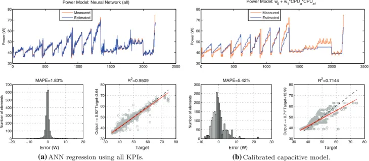
Figure 7 contains the results of the capacitive and the

neural network models. For each model, three subfigures summarize its results. At the top, the estimated (output) and measured (target) powers are plotted side by side, to verify that the model is really capable of predicting the data. At the bottom left, a histogram of the difference between the mea-sured and estimated power (y− ˆy) provides the distribution of the magnitude of the error along with its MAPE. At the bot-tom right, the correlation between estimated and measured values is shown. It contains the scatterplot of the data and

0 500 1000 1500 2000 2500 30 40 50 60 70 80 Power (W)

Power Model: Neural Network (all)

Measured Estimated −200 −10 0 10 20 100 200 300 400 500 600 700 Number of elements Error (W) MAPE=1.83% 30 40 50 60 70 80 30 40 50 60 70 80 Output ~= 0.92*Target+3.64 Target R2=0.9509 0 500 1000 1500 2000 2500 30 40 50 60 70 80 Power (W) Power Model: w 0 + w1*CPUu*CPUaf Measured Estimated −100 0 10 20 30 50 100 150 200 250 300 Number of elements Error (W) MAPE=5.42% 30 40 50 60 70 80 30 40 50 60 70 80 Output ~= 0.71*Target+12.99 Target R2=0.7144

(a)ANN regression using all KPIs. (b)Calibrated capacitive model.

two reference lines. The dashed line represents the perfect data fit, while the continuous one is the linear regression of the data; the closer they are, the better.

One can see from Fig.7a that ANN estimation and the

measured values almost overlap, presenting a high preci-sion for the TS’s prediction. The histogram shows that the errors are concentrated near 0 W and the MAPE is low (1.83 %). The correlation of 0.95 means that the ANN is capable of explaining the behaviour of the measured

val-ues. In Fig.7b, the results from the capacitive model after

calibration clearly show that the lack of information regard-ing the use of the processor’s components makes the capac-itive model unable to estimate the power changes between the different µ-benchs (CU, FPU and Rand), reproducing

always the same curve. The results show a MAPE and R2of

5.42 % and 0.71, respectively. The comparison between the two models shows that ANN can provide an estimator more than two times better than the capacitive model.

5.6 Estimation limits

The use of neural networks need that all variables, including the target, used during the training phase covers the entire spectrum of variables’ values; otherwise the estimation will not be accurate. For instance, if the TS’s power range varies from 35 to 75 W, one cannot expect a good prediction of a 100 W configuration set.

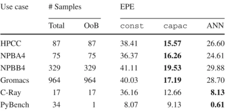
A set of use cases were executed to provide real world application profiles to test our estimator. This set encom-passes several benchmarks: HPC Challenge (HPCC), NAS Parallel Benchmark (NPB), Gromacs, C-Ray and Pybench. HPCC is a set of benchmarks intended to explore the whole spectrum of HPC applications. NPB is a set of linear algebra benchmarks, problem sizes A and B were executed using 4 cores. Gromacs is a molecular dynamics simulator, in this use case, the simulation of DPPC in water was run. C-Ray is a ray tracing benchmark. Pybench is a test set to measure performance of Python programs.

When comparing our synthetic benchmarks with HPC use cases, we noticed that almost every use cases’ samples were

out of the bounds of the training set. Table3presents some

characteristics of the test data, along with the comparison

between three models based on the EPE (Eq.3). One can see

that from the total number of samples of each case, only the PyB has some samples in the bound of the training set, all the other are out of bounds (OoB). This shows that the set of synthetic benchmarks used to generate the TS do not properly represent our HPC use cases. The only use case which the samples were in the same range of the TS (PyB) presented an estimation error of only 0.61 %, for all the other, the ANN had a bad estimation. This shows the importance of the TS for modelling with machine learning. Adaptative learning

techniques can enhance the quality of the TS [3], however

Table 3 Models’ comparison based on several use cases, their total

number of samples and the number of samples that are out of the bounds (OoB) of the training set

Use case # Samples EPE

Total OoB const capac ANN

HPCC 87 87 38.41 15.57 26.60 NPBA4 75 75 36.37 16.26 24.61 NPBB4 329 329 41.11 19.53 29.88 Gromacs 964 964 40.03 17.19 28.70 C-Ray 17 17 36.16 12.66 8.13 PyBench 34 1 8.07 9.13 0.61

The bold values correspond the lowest EPE (Energy Percentage Error) among the 3 models (const, capac and ANN)

it requires the power meter to be continuously available to collect more data.

6 Conclusions

In this paper we introduced the issues of using AC power to create new models, which can generate prediction errors of up to 380 W. Then we pointed out a limitation of CPU proportional estimators. Finally a new methodology for esti-mating the power consumption of computing systems was proposed. While promising, this approach deeply depends on the training set’s quality.

As future work, we intend to generate a broader range of micro benchmarks capable to reproduce HPC application’s profile. Preliminarily results show that the addition of some HPC benchmarks into the training set significantly improves ANN’s estimation. We are also working on the portability of our ANN model to estimate the power dissipated at the process level and distributed systems.

Acknowledgments The results presented in this paper were funded by the European Commission under contract 288701 through the project CoolEmAll.

References

1. Basmadjian R, De Meer H (2012) Evaluating and modeling power consumption of multi-core processors. In: Future Energy Systems (e-Energy), pp 1–10. http://ieeexplore.ieee.org/stamp/stamp.jsp? tp=&arnumber=6221107&isnumber=6221093

2. Bedard D, Lim MY, Fowler R, Porterfield A (2010) Powermon: fine-grained and integrated power monitoring for commodity com-puter systems. In: IEEE SoutheastCon, pp 479–484. doi:10.1109/ SECON.2010.5453824

3. Cupertino LF, Da Costa G, Sayah A, Pierson JM (2013) Energy consumption library. In: Energy efficiency in large scale distributed systems, Lecture Notes in Computer Science. Springer, New York, pp 51–57

4. Diniz B, Guedes D, Meira W Jr, Bianchini R (2007) Limiting the power consumption of main memory. SIGARCH Comput Archit News 35(2):290–301

5. Do T, Rawshdeh S, Shi W (2009) ptop: A process-level power pro-filing tool. In: Power aware computing and systems, HotPower’09. ACM, USA

6. Haykin S (1998) Neural networks: a comprehensive foundation, 2nd edn. Prentice Hall PTR, USA

7. Huang GB (2003) Learning capability and storage capacity of two-hidden-layer feedforward networks. IEEE Trans Neural Netw 14(2):274–281

8. Intel Corporation (2013) Intel 64 and IA-32 Architectures Software Developer’s Manual: System Programming Guide, Part 2 9. Jarus M, Oleksiak A, Piontek T, Wglarz J (2014) Runtime power

usage estimation of HPC servers for various classes of real-life applications. Future Gener Comput Syst 36:299–310. doi:10.1016/ j.future.2013.07.012

10. Mair J, Huang Z, Eyers D, Cupertino LF, Da Costa G, Pierson JM, Hlavacs H (2014) Power modeling. In: Large-scale distributed systems and energy efficiency: a holistic view, vol 5. Wiley, New York (in press)

11. Rivoire S, Ranganathan P, Kozyrakis C (2008) A comparison of high-level full-system power models. In: Power aware computing and systems, HotPower’08, pp 1–5. USENIX Association 12. Volk E, Piatek W, Jarus M, Da Costa G, Sisó L, vor dem Berge M

(2013) Update on definition of the hardware and software models. Tech report, CoolEmAll

13. Weaver V, Johnson M, Kasichayanula K, Ralph J, Luszczek P, Terpstra D, Moore S (2012) Measuring energy and power with PAPI. In: Parallel Processing Workshops (ICPPW), pp. 262–268 14. Willink R (2013) Measurement uncertainty and probability 1st

ed. Cambridge University Press, Cambridge, UK. doi:10.1017/ CBO9781139135085

Leandro Fontoura Cupertino

received his BSc degree in Com-puter Engineering in 2007 from the Rio de Janeiro State Univer-sity (UERJ), Brazil. In 2009 he received MSc degree in Electri-cal Engineering from the Pontif-ical Catholic University of Rio de Janeiro (PUC-Rio). He joined the research group of Toulouse Institute of Computer Science Research (IRIT) in 2012, where he is working on the energy mod-elling of applications. There, he is pursuing a PhD degree in Com-puter Science at the University of Toulouse III, France. His research interests include energy aware computing, cloud and HPC, optimization techniques, computational intelligence and artificial neural networks.

Georges Da Costa is a per-manent Assistant Professor in Computer Science at the Uni-versity of Toulouse. He received his PhD from the LIG HPC research laboratory (Grenoble, France) in 2005. He is member of the IRIT Laboratory. His main interests are related to large-scale distributed systems, algo-rithmic, performance evaluation and energy-aware systems. He is Work Package leader of the Euro-pean project CoolEmAll which aims at providing advanced sim-ulation, visualization and decision support tools along with blueprints of computing building blocks for modular data center environment. He is working group chair of the European COST0804 Action on ’Energy efficiency in large scale distributed systems’. His research currently focus on energy aware distributed systems. He serves on several PCs in the Energy aware systems, Cluster, Grid, Cloud and Peer to Peer fields. His research highlights are grid cluster & cloud computing, hybrid com-puting (CPU/GPU), large scale energy aware distributed systems, per-formance evaluation and ambient systems.

Jean-Marc Pierson serves as a Full Professor in Computer Science at the University of Toulouse (France) since 2006. He received his PhD from the ENS-Lyon, France in1996. He was an Associate Professor at the University Littoral Cote-d’Opale (1997-2001) in Calais, then at INSA-Lyon (2001-2006). He is a member of the IRIT Laboratory and Chair of the SEPIA Team on distributed systems. His main interests are related to large-scale distributed systems. He serves on several PCs and editorial boards in the Cloud, Grid, Pervasive, and Energy-aware computing area. Since the last years, his researches focus on energy aware distributed systems, in particular monitoring, job place-ment and scheduling, virtual machines techniques, green networking, autonomic computing, mathematical modeling. He was chairing the EU funded COST IC804 Action on “Energy Efficiency in Large Scale Distributed Systems” and participates in several national and european projects on energy efficiency in large scale distributed systems. For more information, please visithttp://www.irit.fr/~Jean-Marc.Pierson/.