HAL Id: halshs-00456202
https://halshs.archives-ouvertes.fr/halshs-00456202
Submitted on 12 Feb 2010
HAL is a multi-disciplinary open access archive for the deposit and dissemination of sci-entific research documents, whether they are pub-lished or not. The documents may come from teaching and research institutions in France or abroad, or from public or private research centers.
L’archive ouverte pluridisciplinaire HAL, est destinée au dépôt et à la diffusion de documents scientifiques de niveau recherche, publiés ou non, émanant des établissements d’enseignement et de recherche français ou étrangers, des laboratoires publics ou privés.
Accruals in High Tech Industries
Charlotte Disle, Ignace de Beelde, Rémi Janin
To cite this version:
Charlotte Disle, Ignace de Beelde, Rémi Janin. Accruals in High Tech Industries. La place de la dimension européenne dans la Comptabilité Contrôle Audit, May 2009, Strasbourg, France. pp.CD ROM. �halshs-00456202�
ACCRUALS IN HIGH TECH INDUSTRIES
Charlotte DISLEMaître de conférences, IAE, Université Pierre Mendès France
Membre du CERAG UMR 5820 CNRS/Université Pierre Mendès-France Ignace De BEELDE
Professeur
Université de Gand
Grenoble Ecole de Management Rémi JANIN
Maître de conférences, Université Pierre Mendès-France,
Membre du CERAG UMR 5820 CNRS/Université Pierre Mendès-France
I.A.E de Grenoble, Université Pierre Mendès France, Domaine universitaire, B.P. 47, 38040 Grenoble, Cédex 9 – France
Résumé : Les sociétés de haute technologie européennes, de par leurs caractéristiques (dépenses en actifs immatériels, croissance, innovation…) sont amenées à publier des régularisations comptables. Ceci peut affecter la persistance de leurs résultats. Néanmoins, notre étude indique qu’au global, les résultats des entreprises de haute technologie ne sont pas moins persistants.
Mots clés : haute technologie, persistance du résultat, régularisations comptables
Abstract : The European high technology companies, due to their characteristics (spending in intagible assets, growth, innovation…) tend to publish accruals. This can affect the persistance of their earnings. Nevertheless, our study shows that in the global, the results of the high technology companies are not less persistent.
Key words : high tech, earning persistance, accruals
INTRODUCTION
There is an extensive literature on the usefulness of accruals versus cash flows. A specific topic in these papers is the persistence of accruals and cash flows. In this paper, we investigate whether there are differences between high tech and low tech companies with respect to persistence of components of earnings in a European context. The increasing importance of intangibles is regarded as a potential explanation of a decrease of the value relevance of accounting figures. This is mainly the case in a US context where almost all intangibles are expensed immediately. Traditionally, European companies were allowed to capitalize more intangibles than US companies. As high tech companies generally are considered to have significant intangible assets, we compare European listed high tech companies with European listed low tech companies, to find out whether these companies show systematic differences with respect to the persistence of accruals and cash flows. High tech companies are also considered as having a more volatile environment and are consequently likely to disclose more variable accruals. Our results show that over the period 2001-2005, there are no significant differences between both types of companies with respect to total, short term and long term accruals. However, a year by year analysis shows a strong volatility of the accruals of high tech companies, mainly due to the impact of the high tech crisis in 2001 and 2002. In these years, the results for high tech companies are significantly different from those for low tech companies, suggesting that economic circumstances in the industry can have a significant impact on accruals persistence.
1. PERSISTENCE OF ACCRUALS AND CASH FLOWS
To be useful, accrual and cash-flow components of current earnings must convey relevant information for investor decision making. The literature on the usefulness of accounting figures provides evidence that accrual accounting earnings are superior to cash-flows to convey information about firm performance (Dechow, 1994). Indeed, accrual based accounting figures allow a registration of transactions that did not yet result in incoming or outgoing cash flows, but that already resulted in the creation or destruction of value. However, Sloan (1996) has demonstrated that accruals are less persistent than cash flows in 86 percent of the industries he examines and consequently are less informative with respect to future earnings. Subsequent research has extended Sloan’s work by providing new evidence of why accruals are less reliable. Xie (2001) shows that abnormal accruals (measured using the Jones, 1991, model) are those that are less persistent. Xie attributes the weak persistence of abnormal accruals to their discretionary component. Dechow and Dichev (2002) show that the weak persistence of accruals is linked with their quality. They assume accruals that do not match with past, present, or future cash-flows to be of lower quality. Richardson et al. (2005) confirm that lower quality accruals are less persistent and so less useful for predicting future earnings. Their analysis includes accrual categories that were not investigated in previous research and that sometimes have very low reliability. Dechow and Ge (2006) concluded that the application of the matching principle in accounting explains why high accruals firms have higher earnings persistence than low accruals firms. They provide evidence that low accruals firms report less persistent earnings because they record temporary special items resulting
from large accrual adjustments for impairments or restructuring charges. Fairfield et al. (2003) link the lower persistence of accruals with the level of investment. They show that, for firms with similar return on assets in year t, firms investing relatively more in net operating assets experience lower profitability in t+1. Similar results were obtained by Titman et al. (2004) and Anderson and Garcia-Feijoo (2006). Dechow et al. (2008) decompose the cash component of earnings and conclude that the higher persistence of the cash component is entirely due to the subcomponent related to equity financing activities. Cash flows related to debt transactions or changes in the cash balance have low earnings persistence similar to accruals.
In 1999, Lev and Zarowin have shown that the usefulness of earnings has much declined over the last decades. They argue that this decline is mainly due to the increasing importance of intangible assets and the inadequate accounting treatment of this change and its consequences. The objective of this paper is to examine whether the persistence of accrual and cash-flow components of current earnings is affected by the level of intangibles, using a sample of European high tech companies. We focus on high tech companies because most of them have a larger portfolio of intangible assets than low tech companies.
Intangibles intensity affects the persistence of long term accruals and short term accruals in different ways. High tech companies are likely to report specific long term accruals linked to investments in intangible assets. These accruals might behave differently from the accruals related to other assets. Obviously, if all intangibles are expensed immediately, they have an impact directly on operating income rather than on accruals. However, also in the US context where most intangibles are unrecognized in the balance sheet, the characteristics of the financial statements of US high tech companies are different from those of low tech companies: Kwon, Yin and Han (2006) show that US high tech companies are more likely to use conservative accounting methods than US low tech companies. Our data relate to European companies that, before the adoption of IFRS, had an option to capitalize a range of intangibles and their amortization or depreciation.
Mandatory capitalizing of specific intangibles increases the usefulness of financial statements, as is demonstrated in an Australian context where Matolcsy and Wyatt (2006) find that capitalization of intangible assets is associated with lower earnings forecast error by analysts. Investigating how to improve US GAAP, Lev and Sougiannis (1996), Aboody et Lev (1998) and Zhao, (2002) studied the relevance of accounting figures in case of the capitalization of intangible assets and show that capitalization improves relevance. If intangibles are capitalized, earnings for firms with high intangibles are less seriously affected by mismatching intangible expenditures against revenues (Choi and Lee, 2003). Capitalizing some intangible assets generates specific long term accruals, including depreciation or amortization, which could improve the ability of accruals-based earnings measures to convey relevant information about firm value. However, these benefits of accrual measures may be offset by potential opportunistic choices of managers. Kwon, Yin and Han (2006) provide evidence that high tech firms are more likely to take income-decreasing earnings management decisions, in comparison with low tech firms. This kind of managerial intervention may alter the quality and persistence of accruals (Dechow and Dichev, 2002).
A relative uncertainty of revenues and earnings arises from investments in intangibles. Hence, many high tech companies with high intangibles can be expected to have specific economic characteristics and show a specific accounting behaviour which affects the usefulness of their financial statements, as they have an atypical business model without an historical pattern of regular profitability. This uncertainty of future benefits is generally higher for investments in intangibles than for more traditional investments. Kothari, Laguerre and Leone (2002), for example, provide evidence that on average R&D investments generate future benefits about three times more variable compared to capital expenditures. High tech companies with high intangibles have a volatile operating environment and are consequently likely to have a less stable and predictable performance than low tech companies. Firm growth also has an impact on accruals. A firm that is growing will be a firm that, ceteris paribus, is recording positive working capital accruals (short term accruals). In contrast, a firm that is recording declining revenues will also report, ceteris paribus, negative working capital accruals. As pointed out by Francis and Krishnan (1999), the more reported earnings diverge from cash flows, the greater the risk that earnings contain undetected estimation errors (intentional or otherwise) and, therefore, potential valuation errors. Large sales volatility induces a greater magnitude of short term accruals, and, therefore, reduced persistence.
In summary, we investigate whether the accruals disclosed by high tech companies are more or less persistent than accruals disclosed by low tech companies. We consider that it is necessary to distinguish long term and short term accruals. Given that European accounting rules allowed or even required capitalization of intangibles in a broader range of cases, we expect that high tech companies do not differ from low techs with respect the persistence of long term accruals. As high tech companies have a more volatile operating environment and more variable revenues, we conjecture that high tech firms book less persistent short term accruals than low techs. This results in the following hypotheses being tested.
H1 : The persistence of long term accruals of both high tech and low tech firms is the same. H2 : High tech firms have less persistent short term accruals than low tech.
2. VARIABLE MEASUREMENT AND HIGH TECH DEFINITION
The variables that we use in this study are earnings, total accruals, short term accruals, long term accruals and cash from operations. In order to exclude non-recurring items, earnings are defined as operating income after depreciation. Following prior research (Subramanyan, 1996 or Xie, 2001), total accruals (TA) are calculated with the balance sheet formula :
ΤΑ = (ΔCA– ΔCash) – (ΔCL – ΔSTD) – Dep where ΔCA = change in current assets
ΔCash = change in cash and cash equivalents ΔCL = change in current liabilities
Dep = depreciation and amortization expense
For the empirical analysis, all variables are standardized by total assets. Depreciation and amortization expense corresponds to long term accruals (LTA) and short term accruals are the sum of total accruals and long term accruals; i.e., STA = TA + LTA = (ΔCA– ΔCash) – (ΔCL – ΔSTD).
Operating cash flow (CFO) is measured as the difference between earnings and total accruals : OCF = Earnings – TA
Distinguishing high tech from low tech firms is not easy. Grinstein and Goldman (2006) summarized the definitions that can be found in the literature and concluded that many of them are arbitrary and simplistic. They found that technology firms differ from others in their positioning on three dimensions: R&D activity and the organizational elements and market conditions associated with it, a corporate culture of innovativeness and entrepreneurship, and an open and informal corporate culture. Thornhill (2006) categorized industries as high or low tech based on R&D intensity and on the percentage of knowledge workers. High tech firms were more dynamic and innovative. Chen and Williams (1999) used a similar approach. They identified four low technology and five high technology industries based on occupational mix and R&D. The industries were identified on a 2-digit SIC level. A main weakness of using this method is that it assumes that all firms in an industry have similar characteristics. If industries are heterogeneous with respect to their technological level, this introduces errors in the analysis.
Data using workforce characteristics are often not available from public sources. The US accounting practice of immediately expensing most intangibles also limits information on R&D activities in the financial statements. Some studies therefore use a more straightforward classification or just take one or two industries of which one is (rather intuitively) considered to be high tech while the other is supposedly low tech. An example of this approach is Karakaya and Kobu (1994), who compare the medical instrument technology industry and the food processing industry. Barron et al. (2002) identified a number of high tech industries based on 3-digit SIC codes.
In this paper, we refer to the sectorial classification proposed by Francis et Schipper (1999) to distinguish between high and low tech industries. Following their classification, we considered the following US SIC codes as representing high tech industries: 28 (Chemicals and allied products manufacturing), 35 (Industrial and commercial machinery and computer equipment), 36 (Electronic and other electrical equipment and components, except computer equipment), 48 (Communications), 73 (Business services) and 87 (Engineering, accounting, research, management and related services). High tech industries are characterized by heavy investment in intangibles and by substantial spending on the development of customer-base and market share (Amir and Lev, 1996). To take this into account, we refined the classification and calculated quartiles on the ratio intangible assets/total assets for both high and low tech industries. We included companies in the three last quartiles in the SIC 28, 35,
36, 48, 73 and 87 industries in our high tech sample, and companies in the first three quartiles in the other industries in our low tech sample.
3. DATA
Data are taken from the Amadeus database. The original sample included all companies listed in Belgium, Finland, France, Germany, Greece, Italy, the Netherlands, Portugal, Spain, Sweden and the United Kingdom for which financial statements were available in the database, excluding those in the financial services, insurance and real estate industries. The original sample included 24172 observations on a 5 year period. We first eliminated all companies with missing data or corrupt data (such as negative total assets). We then eliminated extreme values by excluding the highest and lowest percentile on Operating Income and Operating Cash Flow. Finally we separated high tech and low tech companies and eliminated the quartile in each of the subsamples that came closest to the other subsample. Sample numbers are given in table 1.
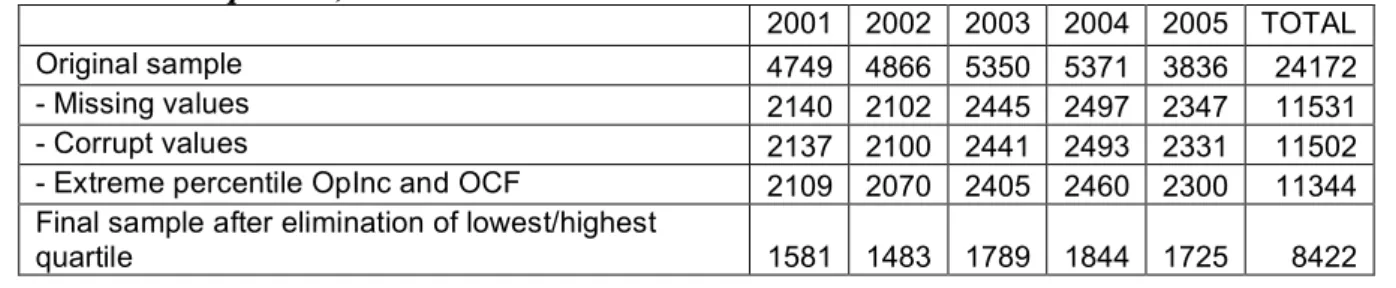
Table 1. Sample size, 2001-2005
2001 2002 2003 2004 2005 TOTAL
Original sample 4749 4866 5350 5371 3836 24172
- Missing values 2140 2102 2445 2497 2347 11531
- Corrupt values 2137 2100 2441 2493 2331 11502
- Extreme percentile OpInc and OCF 2109 2070 2405 2460 2300 11344 Final sample after elimination of lowest/highest
quartile 1581 1483 1789 1844 1725 8422
Table 2 includes descriptive statistics for the final sample by comparing high tech and low tech companies as we have defined them. It reports reported intangibles, Operating Income, Total accruals, Short-term accruals, Long-term accruals and Operating cash flow (all deflated by total assets).
Table 2 : Descriptive statistics high tech (HT) versus low tech (LT)
LT (N=5088) HT (N=3335)
Mean Median Mean Median t-stat z-stat
INT 0,032 0,015 0,239 0,179 -72,997 -64,467 OpInc 0,041 0,054 -0,034 0,034 18,176 -13,804 TA -0,047 -0,042 -0,081 -0,062 10,109 -9,948 STA 0,001 0,003 -0,012 -0,005 4,311 -4,524 LTA 0,048 0,040 0,069 0,050 -15,401 -16,221 OCF 0,088 0,096 0,047 0,086 9,510 -6,259
All average and median values deflated by total assets. Int = Intangibles, OpInc = Operating income, TA = Total accruals, STA = Short term accruals, LTA = Long term accruals, OCF = Operating cash flow
t-stat : t de student pour la comparaison des moyennes de deux échantillons indépendants (corrigé pour l’hétérogénéité de
la variance le cas échéant).
z-stat : le test non paramétrique de Mann-Whitney porte sur l’hypothèse nulle d’homogénéité des distributions.
By definition, high tech companies in our sample have a higher percentage of intangibles. The difference between high and low tech is very significant, with seven to eight times as
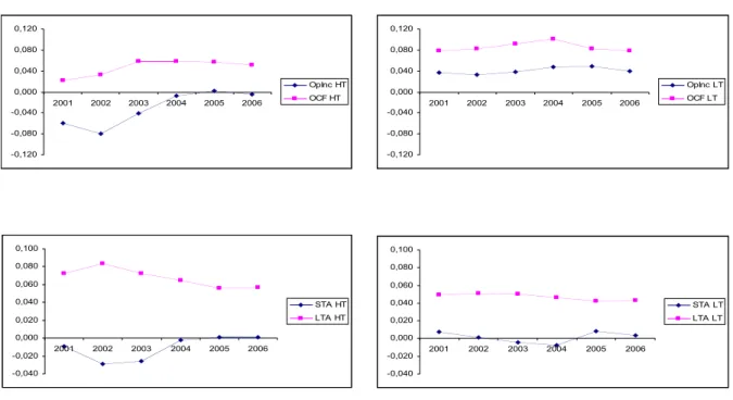
many intangibles. The high tech companies are significantly weaker performers, as can be seen from operating income and cash flow data. They also disclose significantly higher total accruals. This difference between high tech and low tech companies is due to both short term accruals and long term accruals. However, the graphs in Figure 1 show that the accounting characteristics of high tech companies vary across years. More precisely, the graphs underline the impact of the crisis of the high tech industries in the early 2000s. Operating cash flows remained positive in both high and low tech industries, but operating income was quite negative in 2001-2003 for the high tech sample. From an accounting perspective, the high tech crisis mainly reflects on the accruals. Total accruals are very high during 2001, 2002 and 2003. Overall, accruals are negative for the whole period and in both samples. However, they are significantly higher in the high tech sample in 2001, 2002 and 2003. If we separate short term and long term accruals, we observe that long term accruals follow the general pattern: they are higher for high tech companies, especially in 2001, 2002 and 2003. Short term accruals in high tech companies are very different from those in low tech companies during these three years. Both average and median short term accruals are very close to zero in low tech companies, but very negative for high tech companies. This translates a reduction of the net working capital in high tech companies during this period. In 2004-2006, on the contrary, short term accruals are not very different between the two samples.
Figure 1 : Earnings and earnings components of high tech (HT) and low tech (LT) companies over the period 2001-2006
OpInc = Operating income, STA = Short term accruals, LTA = Long term accruals, OCF = Operating cash flow
The percentage of loss firms confirms that the financial performance of high tech industries is more uncertain than that of low techs and that many high tech companies were affected by the
-0,120 -0,080 -0,040 0,000 0,040 0,080 0,120 2001 2002 2003 2004 2005 2006 OpInc LT OCF LT -0,120 -0,080 -0,040 0,000 0,040 0,080 0,120 2001 2002 2003 2004 2005 2006 OpInc HT OCF HT -0,040 -0,020 0,000 0,020 0,040 0,060 0,080 0,100 2001 2002 2003 2004 2005 2006 STA LT LTA LT -0,040 -0,020 0,000 0,020 0,040 0,060 0,080 0,100 2001 2002 2003 2004 2005 2006 STA HT LTA HT
high tech firms (always above 31%, a percentage never attained by the low tech sample). Especially 2001-2003 has higher percentages: more than 40%, with a peak of 45% in 2002.
Table 3: Percentage of firms reporting losses, low tech versus high tech
2001 2002 2003 2004 2005 2006
Loss reporting,
low tech 177 190 218 193 210 169
number low tech 953 934 1078 1103 1020 894
percentage loss
low tech 18,63% 20,34% 20,22% 17,50% 20,59% 18,90%
Loss reporting,
high tech 255 248 301 254 223 201
Number high tech 628 549 711 741 705 646
percentage loss
high tech 40,61% 45,09% 42,33% 34,28% 31,63% 31,11%
4. RESULTS
In line with prior research, we first investigate the persistence of earnings and their components for the whole sample by performing these three Ordinary Least Squares regressions :
Earningst+1 = a0 + a1 Earningst + et+1 (1)
Earningst+1 = b0 + b1 TAt +b2 CF0t + et+1 (2)
Earningst+1 = c0 + c1 STAt + c2 LTAt + c3 OCFt + et+1 (3) where TA = total accruals,
STA = Short term accruals, LTA = Long term accruals, OCF = Operating cash flow
These regressions provide evidence on how well current earnings or its components convey information about future earnings. Coefficients of the regressions give a measure of the persistence. c1 and c3 are expected to be positive, but as long term accruals correspond to charges such as amortization or impairment, c2 is expected to be negative.
Next, we compare the persistence of earnings and their components in High tech versus Low tech firms. Therefore, we introduce in each regression a dummy variable (D) equal to one if the firm is low tech or zero if the firm is high tech :
Earningst+1 = a0 + a1 Earningst + a2 Dt + a3 D×Earningst + et+1 (4)
Earningst+1 = b0 + b1 TAt + b2OCFt + b3 Dt + b4 D×TAt + b5 D×OCFt + et+1 (5)
Earningst+1 = c0 + c1 STAt + c2 LTAt + c3 OCFt + c4 Dt + c5 D×STAt + c6 D×LTAt + c7
If being a high tech company influences the persistence of accounting variables, the coefficients of the interaction with D must be significantly different from zero. For example, a positive coefficient a3 in equation (4) would signify that earnings of low tech firms are more persistent than earnings of high tech firms.
2.1 PERSISTENCE OF OPERATING INCOME
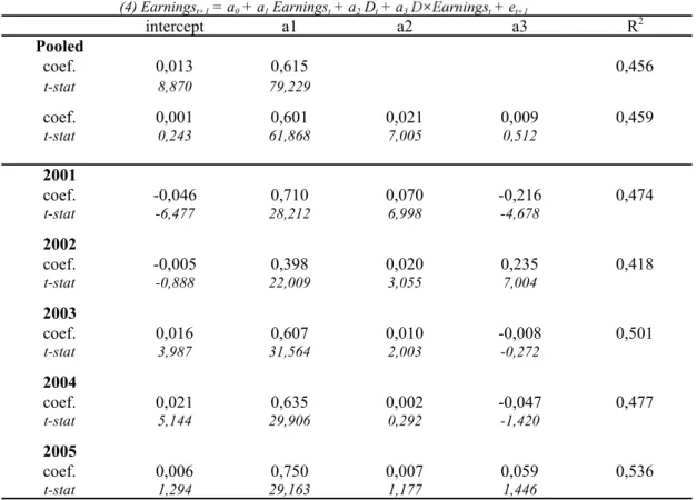
Table 4 : Persistence of operating income, pooled and year by year
(1) Earningst+1 = a0 + a1 Earningst + et+1 (4) Earningst+1 = a0 + a1 Earningst + a2 Dt + a3 t + et+1 intercept a1 a2 a3 R2 Pooled coef. 0,013 0,615 0,456 t-stat 8,870 79,229 coef. 0,001 0,601 0,021 0,009 0,459 t-stat 0,243 61,868 7,005 0,512 2001 coef. -0,046 0,710 0,070 -0,216 0,474 t-stat -6,477 28,212 6,998 -4,678 2002 coef. -0,005 0,398 0,020 0,235 0,418 t-stat -0,888 22,009 3,055 7,004 2003 coef. 0,016 0,607 0,010 -0,008 0,501 t-stat 3,987 31,564 2,003 -0,272 2004 coef. 0,021 0,635 0,002 -0,047 0,477 t-stat 5,144 29,906 0,292 -1,420 2005 coef. 0,006 0,750 0,007 0,059 0,536 t-stat 1,294 29,163 1,177 1,446
Earnings are defined as operating income after depreciation. The dummy variable (D) equals to one if the firm is low tech or zero if the firm is high tech
Table 4 provides results from the estimation of equation (4) in pooled form and year by year. In this paper, we did not formulate any hypothesis about earnings persistence because our focus is on accruals. However, Table 4 is included to be able to compare with other research. The estimation of a1 is 0,615 and the t-statistic strongly rejects that earnings would be purely transitory (i.e., a1 = 0). This is consistent with Sloan (1996), although his results show that US companies report more persistent earnings with a mean measure of persistence equal to 0,841.
A comparison with equation (4) shows that there is no difference between high tech and low tech. The pooled estimate of a3 is not statistically different from zero (0,512). These results suggest that earnings disclosed by high tech companies are not less informative about future
and 2005 for the high tech firms. Earnings persistence is high in 2001, with a1 having a value of 0,710. It reduces strongly in 2002 with a level of 0,398 suggesting that high tech earnings are predominantly transitory. Then, the coefficient grows to a value of 0,750 in 2005. The a3 coefficient is statistically different from zero in 2001 and 2002. Low tech firm earnings are less persistent in 2001 and more persistent in 2002. From 2003 to 2005, there is no statistically significant difference between high and low tech. 2001 and 2002 form an atypical economic period. Many high tech companies faced large losses as illustrated in Figure 1. 2002 was the peak of the crisis. Losses reported in 2001 announced even more important losses reported in 2002. This results in a coefficient of persistence that is high in 2001. The improvement in earnings from 2003 explains the very low persistence of earnings in 2002. As low tech firms were less affected by the dot-com crisis, they show different and more regular earnings persistence coefficients (a1 + a3) than high tech firms.
2.2 PERSISTENCE OF ACCRUALS
Table 5 : Persistence of accruals and cash flows pooled and year by year
(2) Earningst+1 = b0 + b1 TAt +b2 CF0t + et+1
(5) Earningst+1 = b0 + b1 TAt + b2CFOt + b3 Dt + b4 D_ TAt + b5 D_ CFOt + et+1
intercept b1 b2 b3 b4 b5 R2 Pooled coef. 0,011 0,593 0,623 0,457 t-stat 6,887 59,772 77,582 F-test of b1 = b2 : 12,970 coef. -0,003 0,565 0,614 0,024 0,032 0,000 0,460 t-stat -1,298 42,383 60,212 7,327 1,526 0,001 2001 coef. -0,048 0,692 0,718 0,066 -0,256 -0,191 0,474 t-stat -6,274 17,678 25,420 6,178 -4,061 -3,750 2002 coef. -0,005 0,398 0,398 0,022 0,262 0,231 0,417 t-stat -0,813 14,246 21,141 3,056 5,463 6,749 2003 coef. 0,011 0,576 0,626 0,016 0,027 -0,028 0,503 t-stat 2,453 26,496 31,123 2,900 0,816 -0,905 2004 coef. 0,014 0,554 0,661 0,007 0,013 -0,068 0,480 t-stat 3,137 17,613 29,548 1,120 0,273 -1,966 2005 coef. -0,001 0,652 0,759 0,012 0,107 0,057 0,539 t-stat -0,125 17,116 29,510 1,768 1,931 1,403
Earnings are defined as operating income after depreciation. The dummy variable (D) equals to one if the firm is low tech or zero if the firm is high tech. TA = total accruals, STA = Short term accruals, LTA = Long term accruals, CFO = Operating cash flow
Table 5 reports results for equation (2) only in pooled form and equation (5) in pooled form and year by year. The pooled coefficient of total accruals is lower than the coefficient of cash
from operations (b1 = 0,593 and b2 = 0,623). An F-test confirms their statistical difference. This is consistent with Sloan (1996) and confirms that total accruals are less persistent than cash from operations.
Coefficients b4 and b5 are not statistically different from zero in equation (5) supporting that persistence of total accruals and persistence of cash from operations are not different between high tech and low tech companies. The year by year regressions show that results are not stable in time. Except for 2002, total accruals in high tech firms are less persistent than cash from operations. However, in 2001 the persistence of total accruals is high and very close to the persistence of cash flows. The poor earnings in 2002 were announced by the two components of earnings in 2001. 2002 is a turning point, which explains the weak persistence of the two components of 2002 earnings (b1 = b2 = 0,398). After 2002, the persistence of total accruals and cash from operations increases. Compared with low tech companies, the results are quite similar to results presented in Table 4. The persistence of total accruals and cash from operations is different for low tech companies in 2001 and 2002 compared to high tech. In 2001, the two components are less persistent (b1 + b4 < b1 and b2 + b5 < b2). In 2002, the two components are more persistent. Low tech companies were less affected by bad economic conditions in 2001 and 2002. Consequently they reported more stable total accruals and cash from operations. After 2002, there is no statistical difference between high tech and low tech, except for cash from operations in 2004 and total accruals in 2005.
Table 6 : Persistence of short terms accruals and long terms accruals pooled and year by year
(3) Earningst+1 = c0 + c1 STAt + c2 LTAt + c3 CFOt + et+1
(6) Earningst+1 = c0 + c1 STAt + c2 LTAt + c3 CFOt + c4 Dt + c5 D_ STAt + c6 D_ LTAt + c7 D_ CFOt+ et+1
intercept c1 c2 c3 c4 c5 c6 c7 R2 Pooled coef. 0,004 0,617 -0,486 0,634 0,458 t-stat 1,965 55,269 -19,433 75,566 F-test of c1 = c2 = c3 : 34,644 coef. -0,010 0,593 -0,464 0,625 0,022 0,028 0,024 0,001 0,462 t-stat -3,237 38,469 -14,720 58,642 5,110 1,225 0,461 0,037 2001 coef. -0,046 0,683 -0,719 0,716 0,067 -0,256 0,233 -0,193 0,473 t-stat -4,924 14,409 -8,484 24,633 4,804 -3,531 1,474 -3,677 2002 coef. -0,017 0,455 -0,226 0,424 0,010 0,328 -0,052 0,261 0,431 t-stat -2,422 13,548 -3,485 20,636 1,051 5,910 -0,511 7,195 2003 coef. 0,008 0,584 -0,537 0,631 0,012 0,029 0,058 -0,026 0,503 t-stat 1,361 23,848 -9,709 29,884 1,577 0,810 0,590 -0,816 2004 coef. 0,009 0,578 -0,473 0,664 0,006 0,012 0,025 -0,067 0,481 t-stat 1,465 16,232 -7,408 29,543 0,838 0,233 0,253 -1,956 2005 coef. -0,015 0,702 -0,403 0,775 0,028 0,052 -0,395 0,039 0,542 t-stat -2,304 17,172 -4,794 29,689 3,067 0,883 -2,857 0,965
Earnings are defined as operating income after depreciation. The dummy variable (D) equals to one if the firm is low tech or zero if the firm is high tech. TA = total accruals, STA = Short term accruals, LTA = Long term accruals, CFO = Operating cash flow
Results in table 6 allow us to analyse persistence by decomposing total accruals in short term and long term accruals. An F-test statistic indicates that pooled estimates of c1, c2 and c3 in equation (3) are different. Short term accruals are much more persistent than long term accruals (c1 > c2, in absolute value). With a coefficient of less than 0,5, long term accruals, which include items like amortization, impairment or restructuring charges, can be considered transitory. A comparison with equation (6) estimated in pooled form shows that, supporting the H1 hypothesis but rejecting the H2 hypothesis, there is no statistical difference between high tech and low tech companies. Neither long term accruals nor short term accruals seem to have different degrees of persistence between high tech and low tech companies. Nevertheless, 2001 is again very particular for the high tech firms. Long term accruals have the highest persistence (c2 = -0,719) suggesting that some special items booked in 2001 convey relevant information about the poor 2002 earnings. For all other years, long term accruals are less persistent than short term accruals. For three years out of five, the coefficient c2 is even less than 0,5. 2002 is also a particular year, with long term accruals being very transitory (close to 80% (1 – 0,226). Long term accrual adjustments in 2002 show no relation to the situation from 2003 onwards, with its better economic conditions. To compare low tech and high tech companies, the decomposition of total accruals in 2001 is very revealing. With a coefficient c5 of -0,256 and a t-stat of -3,531 in 2001, short term accruals are less recurrent
(see Figure 1). This reduction of net working capital accruals, which induces a decrease of earnings, conveys information about the weak result in 2002. In 2002, the short term accruals of high tech companies are transitory (c1<0,5) and less persistent than those of the low tech sample. The strong reduction of net working capital in 2002 seems unrelated to the improvement of the results in 2003. Contrary to this, low tech firms have very persistent short term accruals (c1+c5 = 0,783). During the following years, there is no significant difference anymore between short term accruals of high techs and low techs.
The coefficient c6 is not statistically different from zero in 2001. This result suggests that long term accruals have the same persistence in both high and low tech firms. In other words, some low tech firms booked also special items as depreciation or restructuring provisions in this period to avoid assets being overstated or liabilities being understated in the balance sheet. In 2002, with c2 equal to - 0,226, the long term accruals are not persistent. The heavy impairment charges that were booked by high techs in 2002 are contradictory to the improvement of the results that can be observed from 2003 onwards (see Table 2). We observe that 2002 low tech, long term accruals are not more persistent than those of the high techs. At the end of the period, long term accruals are transitory, whatever the technology level of the industries, with the exception of low techs in 2005.
CONCLUSION
This paper contributes to the literature comparing earnings and accrual persistence in high and low tech industries. It does so in a context where more possibilities to capitalize intangibles exist: European companies were not required to charge all intangibles to the income statement. High tech industries have more intangibles, and the way these are accounted for has a great impact on reported financial statements. Moreover, High tech industries face to a more volatile environment and are consequently likely to have less stable and predictable accounting performance. Reported figures for high tech companies are expected significantly different from those reported for low techs.
The differences that can be observed between high tech industries and low tech industries concentrate in 2001 and 2002. High techs report higher variability in accruals in 2001 and 2002, and both their short term accruals and long term accruals during this period are very different from those reported by low techs.
The period that we studied was turbulent for high tech companies. The unwinding of the dot-com bubble caused a major crisis in high tech startups in the early 2000s. We see the effect of this in the accounting figures. As losses became deeper during the first years of the period that we studied, results are persistent. The persistence of accruals disappears when the tendency in the industry changes and once the financial conditions in the industry become stable again, the persistence of accruals increases again. In this sense, this research confirms that economic conditions in the industry can have a strong impact on accruals.
Once the worst of the crisis is over, figures stabilize again and differences between high and low tech companies become smaller. The different asset bases for our low and high tech samples, amongst which intangibles are a major component, do not result in differences in accrual persistence once the disturbing effect of the high tech crisis has disappeared.
REFERENCES
Amir and Lev (1996) Value relevance of nonfinancial information: the wireless communications industry, Journal of Accounting and Economics, 22, 3-30.
Anderson and Garcia-Feijoo (2006) Empirical evidence on capital investment, growth options and security returns, Journal of Finance, 61, 171-194.
Asthana and Zhang (2006) Effect of R&D investments on persistence of abnormal earnings, Review of Accounting and Finance, 5, 124-139.
Dechow (1994) Accounting earnings and cash flows as measures of firm performance: the role of accounting accruals, Journal of Accounting and Economics, 18, 3-42.
Dechow and Dichev (2002) The quality of accruals and earnings: the role of accrual estimation error, The Accounting Review, 77, 35-59
Dechow and Ge (2006) The persistence of earnings and cash flows and the role of special items, Review of Accounting Studies, 11, 253-296
Dechow Richardson and Sloan (2008) The persistence and pricing of the cash component of earnings, Journal of Accounting Research, 46, 537-566.
Fairfield Whisenant and Yohn (2003) Accrued earnings and growth: implications for future profitability and market mispricing, The Accounting Review, 78, 353-371.
Francis and Krishnan (1999) Accounting accruals and auditor reporting conservatism, Contemporary Accounting Research, 16 (1), 135-165.
Francis and Schipper (1999) Have financial statements lost their relevance?, Journal of Accounting Research, 37, 319-352.
Grinstein and Goldman (2006) Characterizing the technology firm: an exploratory study, Research Policy, 35, 121-143.
Jones (1991) Earnings management during import relief investigations, Journal of Accounting Research, 29(2), 193-228.
Juntilla Kallunki Kärja Martikainen (2005) Stock market response to analysts’ perceptions and earnings in a technology-intensive environment.International review of financial analysis, 14, 77-92.
Karakaya and Kobu (1994) New product development process: an investigation of success and failure in high-technology and non-high-high-technology firms, Journal of Business Venturing, 9, 49-66.
Kothari Laguerre Leone (2002) Capitalization versus expensing: evidence on the uncertainty of future earnings from capital expenditures versus R&D outlays, Review of Accounting Studies, 7 (4), 355-382.
Matolcsy and Wyatt (2006) Capitalized intangibles and financial analysts, Accounting and Finance, 46, 457-479. Richardson Sloan Soliman and Tuna (2005) Accrual reliability, earnings persistence and stock prices, Journal of Accounting and Economics, 39, 437-485.
Sloan (1996) Do stock prices fully reflect information in cash flows and accruals about future earnings?, The Accounting Review, 71 (3), 289-315.
Thornhill (2006) Knowledge, innovation and firm performance in high- and low-technology regimes, Journal of business venturing, 21, 687-703
Titman Wei and Xie (2004), Capital investments and stock returns, Journal of Financial and Quantitative Analysis, 39, 677-700.
World Bank (2006), Where is the wealth of nations? Measuring capital for the 21st century, Washington: World
Bank)