HAL Id: hal-01846924
https://hal.archives-ouvertes.fr/hal-01846924
Submitted on 8 Nov 2019
HAL is a multi-disciplinary open access
archive for the deposit and dissemination of
sci-entific research documents, whether they are
pub-lished or not. The documents may come from
teaching and research institutions in France or
abroad, or from public or private research centers.
L’archive ouverte pluridisciplinaire HAL, est
destinée au dépôt et à la diffusion de documents
scientifiques de niveau recherche, publiés ou non,
émanant des établissements d’enseignement et de
recherche français ou étrangers, des laboratoires
publics ou privés.
Granular flows down inclined channels with a strain-rate
dependent friction coefficient. Part II : cohesive
materials
Alain de Ryck
To cite this version:
Alain de Ryck. Granular flows down inclined channels with a strain-rate dependent friction
coef-ficient. Part II : cohesive materials. Granular Matter, Springer Verlag, 2008, 10 (5), p.361-367.
�10.1007/s10035-008-0106-2�. �hal-01846924�
Granular flows down inclined channels with a strain-rate dependent
friction coefficient. Part II: cohesive materials
Alain de Ryck
Abstract A strain-rate dependent rheology for granular materials with a constant cohesion, is proposed and applied in the case of a flow down an inclined channel. The results obtained show that a plug flow zone appears below the free surface and show that low cohesion may affect drastically the flow behaviour when the inclination of the channel is close to the repose angle. These results give also a basic unders-tanding of hstop, the depth of the remaining granular layer on
an inclined channel, treating dilatancy like a cohesion-like behaviour.
Keywords Granular materials · Cohesive materials · Surface flows
1 Introduction
Humid or fine granular materials exhibit a reduced flowability as soon as the attractive forces between particles become greater than their weight. The consideration of their flow behaviour is of significance for a better design of industrial processes or for the understanding of some geological flows like humid snow avalanches.
To study quantitatively the effect of cohesion in the par-ticular case of a flow on an inclined channel, we present
A. de Ryck (
B
)École des Mines d’Albi, UMR CNRS 2392, Route de Teillet, 81000 Albi, France
e-mail: [email protected] A. de Ryck
Centre for Simulation and Modelling of Particulate Systems, School of Materials Science and Engineering,
The University of New South Wales, Sydney, NSW 2052, Australia
here an extension of the semi-analytical description given in the Part I joint paper [4]. The granular material exhibits a coefficient of friction which depends on the inertial number
I = √| ˙γ|dP/ρ[2,7], and a residual constant cohesion c during flow. P = σii/3 is the mean pressure, σ is the stress ten-sor. d is the diameter of the particles, ρ the bulk density, ˙γ is the strain rate tensor and | ˙γ| = !˙γi j˙γi j/2 its second invariant.
This may be considered as a first simplified approach for cohesive materials since the cohesion term is not expected to be constant. The strength at yield is dependent on the consoli-dation of the material [12], and close to zero when the system is at the so-called critical state [13]. Recent numerical experi-ments by Rognon et al. [10] suggest an another rheology for cohesive materials, where there is no cohesion term, but the friction coefficient increases dependently on two numbers, the inertial number I , and the cohesion number η = fmax
Pd2,
where fmaxis the maximal value taken by the attractive forces
between particles.
With this constant cohesion term, the stress-strain relation then writes:
σi j = −Pδi j+ (c + µ(I)P) ˙γi j
| ˙γ|. (1)
We set-up the equations for a steady-state gravitational flow along an incline in Sect.2, then the constant friction solution is discussed in Sect.3, and the general solution in Sect.4.
2 Mathematical formulation
If we consider the same geometry than in the non-cohesive case (see Fig. 1 in [4]), the Navier–Stokes equations for a steady-state flow writes:
− →∇ · ⎛ ⎝ P 0 (c+ µP) sin α 0 P (c+ µP) cos α (c+ µP) sin α (c + µP) cos α P ⎞ ⎠ = −ρg ⎛ ⎝ 0 cos θ sin θ ⎞ ⎠ , (2)
where α is the local angle made by the iso-velocity line with respect to the x-axis.
These equations lead to a hydrostatic mean pressure:
P= ρg cos θy, (3)
and to a momentum equation along the z-axis which writes: ∂
∂x((c+µP) sin α)+ ∂
∂y((c+µP) cos α)−ρg sin θ =0,(4) where q= P/ρg.
In the following sections, this system will be integrated with a non-slip condition at the walls (w = 0 for x = ±a) and a free surface (α|y=0=π2). First, the case of a constant
coefficient of friction will be considered (Sect.3), then the more general case will be developed (Sect.4).
3 Constant friction
With the hypothesis of constant friction, Eq.4reduces to: (ℓs+ y) & cos α∂α ∂x −sin α ∂α ∂y ' + cos α − R = 0, (5) where ℓs = c µρgcos θ (6)
is a cohesive length and R = tan θµ . This equation can be
integrated as an ordinary differential equation along a s-parametred curve: dx ds =cos α(ℓs+ y), (7) dy ds = −sin α(ℓs + y), (8) dα ds = R− cos α. (9)
Such a curve can be integrated from the point (0, h) for which we have α= 0.The integration of the system (Eqs.7,8and 9), using the same method than presented in the Annex 1 of the companion paper [4], leads to the following parametric equations for the iso-velocity curve:
x= (h + ℓs) s+ R k sin(ks) 1+ R , (10) y+ ℓs = (h + ℓs)R+ cos(ks) 1+ R , (11) where k=√R2− 1.
The solution is similar to the one obtained for a non cohe-sive powder, with the exception that the y-co-ordinates are shifted by ℓs. This leads to more flow patterns.
If the slope of the incline is less than µ, then k is a pure imaginary number and the iso-velocity is curved downwards, then collide the wall, and the conclusion is that w= 0 eve-rywhere.
If the slope of the incline is greater than µ, then the iso-velocity lines are curved upwards. They touch the free surface if y= 0 is solution of the Eq.11, which leads to the condition:
h
ℓs ≤
2
R−1. In such the case, the iso-velocity lines arrive at the surface with an angle α|y=0given by:
cos α|y=0= 1 − h
ℓs(R− 1). (12)
From this equation, we conclude that only the iso-velocity line starting at the depth h= ℓs
R−1presents no stresses at the free surface. Then there is no steady-state flow solutions. We even not have the solution which consists to the sliding of two rigid bodies at the interface given by this particular iso-velocity line since the forces are not balanced.
4 Strain-rate dependent friction coefficient
With an I -dependent coefficient of friction, the parametred equations for an x-symmetric iso-velocity line passing through the point (0, h) may be obtained the same way than for the non-cohesive case [4]. This leads to:
dx ds =cos α(µsℓs+ µy), (13) dy ds = −sin α(µsℓs+ µy), (14) dα ds =tan θ− µ cos α − dµ d II & By h − 1 2cos α ' . (15) where B = hφ′(h)
φ (h), φ being the velocity gradient at x = 0 along the y-axis and the prime a derivation towards y.
These equations may be integrated once to obtain:
dx ds =µsℓs+ µ(h)h + (y − h) tan θ − B h y ( h dµ d I I ydy, (16) &dy ds '2 = (µsℓs+ µy)2− &dx ds '2 . (17)
In order to have an iso-velocity line going to free surface, we must have: dx ds ) ) ) )y =0= 0, (18)
which gives the following value for B:
B= hhtan θ*− µ(h)h − µ0 sℓs
h dµd II ydy
. (19)
With ℓs = 0, we retrieve the result obtained in [4].
To attain the surface, the curvature of the iso-velocity line must be oriented upwards, which gives a maximum value
Bmaxfor B given by: Bmax= 1 2 + tan θ+ − µ(h) dµ d II , |y=h , (20)
Equation19may be integrated in order to obtain the admis-sible velocity profiles. For the next steps of resolution of these equations, we will follow the same scheme developed in [4], with the same µ(I ) relation:
µ(I )= µs+ Iµ2
o
I + 1
, (21)
with Io= 0.28, µs = 0.38, and µ2= 0.64. The equations
are made dimensionless by scaling the lengths with λ = (I φd o√gcos θ) 2, leading toIo I = √ Y, where Y = λy. ψ is defined as in [4] by H = e−2ψ. We then have B=12+ddψln h.
The Eq.19gives an ordinary differential equation for ψ, which has been integrated for several values of the parameter
h
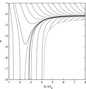
ℓs. A set of results are given in Fig.1in continuous lines. The dashed line borders a zone where there is no valid solution since B > Bmaxin it. We observe that the behaviour for large htends to the one computed for a non-cohesive powder: ψ tends to a constant ψ∗and therefore the velocity gradient at
the centerline behaves like a Bagnold one (φ∝ −√h). This means that the behaviour of large scale flows of cohesive materials (compared to the cohesive length ℓs) is similar to the flow of a non-cohesive material.
4.0.1 Plug flow
For small h, ψ diverges positively or negatively. In the first case, it leads to non-physical solutions since the velocity gradient diverges for a finite value of the depth. In the second case, the velocity gradient φ∝√heψtends to zero for a finite
value of h. These solutions are the ψ-lines which are located between the thick and thin dashed lines in Fig.1. Such a plug flow behaviour has been recently observed in numerical and physical experiments of cohesive granular flows down an incline [1,11].
These feasible solutions end to a plug zone at a depth hplug,
which is bounded by: 1 < hplug ℓs (R− 1) < 2−m 2 1−m 2 . (22)
The upper limit is obtained by looking the limit behaviour of the equality B= Bmax, when φ goes to zero. It is written
Fig. 1 ψ ∝ log√φ
h versus log( h
ℓs), for θ = 22.6◦and µ given by
Eq.21. Continuous lines profiles for different initial conditions. When
h → ∞, then we recover the non-cohesive behaviour and ψ → ψ∗.
Thin dashed lineborderline for the existence of iso-velocity lines curved
upwards; the asymptote for this thin dashed line is h
ℓs = 3/(R − 1).
Thick dashed linelimit between positive or negative divergence for ψ; the asymptote for this thick dashed line is h
ℓs = 1/(R − 1). Thick line
equilibrated profiles
in the generic case where m is the power-law exponent cha-racterizing the behaviour of the coefficient of friction versus the strain rate when this strain rate tends to zero (µ(I ) I∼
→0
µs + Im). In the case of Eq. 21[7], or from the observa-tions by Da Cruz et al. [2] or Rognon et al. [10], we have
m= 1. Hatano et al., from numerical results and theoretical considerations, derive µ(I )∼I15 [6].
Among these solutions, there is only one for which the force balance at the boundary of the plug zone is respected. The Appendix gives the value hplugof the plug flow depth
for this unique solution. It scales with the cohesive length ℓs and only depends on the ratio R between the slope of the incline and the static coefficient of friction. Figure2gives this depth hplug, scaled byRℓ−1s versus the relative difference between the slope and the static coefficient of friction (conti-nuous line). In the same figure, the dashed line gives the ratio between the depth and the half-width xplugof this plug zone.
The asymptotic behaviour for the depth of the plug zone when the inclination angle tends to the repose angle is:
hplug −→
R→1
3
2Rℓ−1s . There is also a maximum limit for the incline slope above which there is no more equilibrated solu-tion within the range given by Eq. 22. Figure 3 gives the limit ratio Rlim we obtain for each value of m between 0
and 2 (continuous line), and the plug depth scaled by ℓs
R−1 (dashed line). We observe in this figure a divergence for
Fig. 2 Continuous line depth of the plug zone hplug, scaled by Rℓ−1s
versus the relative difference between the slope and the static coefficient of friction; Dashed line hplugscaled by the half width of the plug zone
xplug
Fig. 3 Maximal value for steady-state flow Rlimfor the slope scaled
by the static coefficient of friction versus the exponent m (continuous
line) and the plug depth hplugscaled by Rℓ−1s at this limit (dashed line)
m = 2, which corresponds to a shear friction going to a constant value when the mean pressure goes to zero (µP −→P
→0 cst). The coefficient of friction diverges at low
pressure and the the friction shear stress presents a threshold value. The other constraint for the incline slope is that it should remain below µ2, the maximum value of µ(I ).
Fig. 4 ψ Vertical velocity profile at x = 0 for θ = 22.6◦, µs =
arctan(20.9◦)and µ2= arctan(32.6◦). Continuous lines non-cohesive
case (lower) and cohesive case (upper, ℓs= 0.02a). Dashed lines: Slip
velocity at wall: non-cohesive case (lower) and cohesive case (upper). The circles gives the beginning of the matching (w= w(±a, 0)). The
squaregives the end of the plug flow
4.0.2 Matching with slippage at the walls
Finally, the flow layer composed by the iso-velocity lines going to the free surface is matched with the flow layer formed by the iso-velocity lines going to the walls, like in the non-cohesive case [4]. We have also chosen the rough walls boundary conditions to obtain the flow profile given in Fig.4, which compares the depth velocity profiles at the center (continuous lines) and at the walls(dashed lines). The lower curves describe the non-cohesive behaviour and the upper curves are for a cohesion corresponding to a cohesive length ℓs = 0.02a, where a is the half-width of the channel. The inclination of channel is θ = 22.6◦and µ(I ) is given by Eq.21.
The consequence of the cohesion is to reduce the velocities and to create a plug flow under the surface. This behaviour is noticeable including for cohesive lengths small compared to the size of the channel. In the case of Fig.4, the cohesive length c/ρg is more than one hundred times lower than the width of the channel.
5 Discussion
The introduction of a constant cohesion in the rheology des-cribed in [7] has led to modified velocity profiles compared to the ones obtained with no cohesion. Below the free surface,
we have a plug flow of depth proportional to the length c
ρg, with a constant of proportionality (cos θ(tan θ− µs))−1 which diverges when the slope of the incline approaches the angle of repose.
5.1 Remaining cohesion during flow
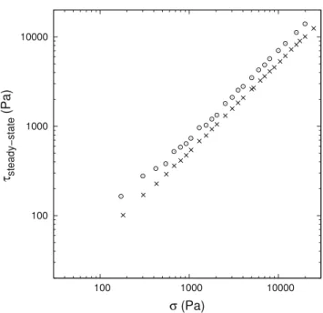
The constant cohesion hypothesis is a crude approximation since it is observed a huge decrease of the strength when the flow starts and the existence of a remaining cohesion during flow remains to be assessed [13]. To check that point, we have performed some yield and steady-state shear experi-ments of dry and wetted glass beads of diameter 200 µm. The beads have been wetted by poly-ethylene glycol (PEG) of molecular weight 200 g with a volume ratio of 1.5%. In our experiments, the cohesion number η is < 5.
The shear stress at steady-state versus the normal stress is displayed on Fig.5for both beads. The dry beads (crosses) have a cohesion-less behaviour with a shear stress propor-tional to the normal stress. The wet beads, which have a cohesion around 500 Pa at yield (not shown) do not present a measurable cohesion at steady-state (see circles in Fig.5). There is a slight shift between the two curves indicating that the friction coefficient of the wetted beads is higher than the friction coefficient of the dry ones. We also observe a slight curvature at low stresses on the τ –σ curve for the wetted beads indicating that, if there is a remaining cohesion, its order of magnitude is lower than 100 Pa. Such a low value gives cohesive lengths ℓs around a few millimeters and we do not expect consequences on the flow behaviour when this flow occurs at a much larger scale. Nevertheless, if the depth of the plug flowscales with ℓs, the coefficient of proportiona-lity 1/(tan θ− µs)diverges when the inclination of channel approaches the angle of repose. The consequence is that very small cohesion may have a measurable effect on the flow at the threshold of sliding on an incline. In Fig.4, the surface velocity is divided by a factor of 2 for a cohesive length 70 times lower than the width of the channel and 1.7◦of
diffe-rence between the repose angle and the channel inclination. This situation corresponds to a 20 cm width channel for our wetted glass beads. As a conclusion, flows in inclined chan-nels are very sensitive to low cohesions when their slopes are close to the static coefficient of friction, the so-called repose angle. This behaviour may become a convenient tool to estimate them.
5.2 Cohesion-like dilatancy
This constant cohesion modeling may also be applied for a non-cohesive material with dilatancy effects in order to obtain hstop, the thickness of the remaining granular layer on
an incline [9]. This cohesion-like term should be the specific energy dissipated to maintain the dilated state and scales:
Fig. 5 Steady-state shear stress versus the normal stress for dry (crosses) and wet glass beads (circles) of diameter 200 µm. 15 ml/l of poly-ethylene glycol of molecular weight 200 g have been used for these experiments
c≃ρg cos θ∆, (23)
where ∆ is the displacement of the barycentre normal to the flow direction. A rough estimate of this length is that it scales like the size of the particles and should vanish when the slope of the incline approaches the maximal value for µ(I ).
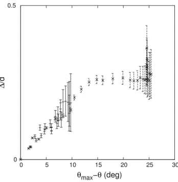
To validate this hypothesis, we have calculated the quan-tity:
∆
d =µs hstop/d
hplug/ℓs. (24)
In Eq.24, the numerator is taken directly from the experi-mental data by Forterre and Pouliquen [5] and Daerr and Douady [3]. The denominator comes from Eq. 26 in the Appendix, with R being built from the experimental slope of the incline divided by µs, the coefficient of friction when
hstopgoes to infinity.
The results are plotted in Fig. 6 versus the difference between the inclination angle and its maximal value. The error bars come from the fact that the determination of µs is within 1◦ of angle precision. We observe first that ∆ is
experimentally of order the size of the beads used. We also observe that the behaviour, for inclination angles close to the maximal value, is similar for both experiments. Despite the approximations used, we obtain a good evaluation for the minimal thickness of the remaining layer of particles in an incline with this cohesion-like behaviour for dilatant granular
Fig. 6 hstop/dexperimental data by Forterre and Pouliquen [5] (plus
symbol) and Daerr and Douady [3] (cross) scaled by hplug/ℓsversus
the difference between the inclination angle and its maximal value. The
error barsrepresents an incertitude of 1◦in the determination of µs
materials. The fact that the rheological model is written for non-dilatant granular materials has a low impact because the flow is non-confined, then the mean pressure remains similar with or without dilatancy and the previous heuristic argu-ments remain valid.
A final remark is that a flow of non-cohesive material should also exhibit a plug flow below the free surface, but such a behaviour has not been reported. To explain that point, we may calculate the plug flow depth at the onset of flow in the case of a coarse wall.
At the onset of flow, the plug invades all the width of the channel, therefore xplug = a, and the Eqs.27and26give
implicitely the depth of the plug zone honset, scaled by the
size d of the particles, using ℓs = 0.25µds. The result is shown in Fig.7using Eq. 21and a
d = 5, 50, 500 and 5,000 from bottom to top. We observe that, as soon as the inclination angle exceed by 3◦the onset inclination angle, the depth of
the plug flow is lower than a tens particles. As a conclusion, this plug flow, for a non-cohesive granular material remains small, except close to the onset of flow. It may be added that the transition between the plug and the flow below it may be softened by some creep motion, as observed by Komatsu et al. [8]. Such a creep not taken into account by the rheology employed.
6 Concluding remarks
The introduction of a constant cohesion in the rheology des-cribed by Eq.1leads to a modified flow pattern compared to
Fig. 7 hplug/dversus the difference between the inclination angle and its value at the onset of flow. µ is given by Eq.21. From bottom to top, the width of the channel is 10, 100, 1,000 and 10,000 d
the non-cohesive case. We obtain a plug flow under the free surface. Its size scales like the cohesive length ℓs, given by Eq.6, times the inverse of the relative ratio between the slope of the incline and the static coefficient of friction. In order to obtain a flow, the depth and width of the powder bed must be greater than this typical length.
The flow behaviour is then highly sensitive to small cohe-sion values when the inclination angle is close to the angle of repose.
From the observation of this behaviour, we hypothesize that the dilatancy effects of non-cohesive materials may be taken into account by the rheological model with a cohesion whose order of magnitude corresponds to a cohesive length of the same order of size than the particles. This prohibits flows at a size scale lower than the size of the particles and gives hstop, the thickness of the remaining layer of grains on
an incline, to diverge when the inclination angle approaches the angle of repose.
Acknowledgments The author takes the pleasure to thank Haiping Zhu and Aibing Yu for fruitful discussions.
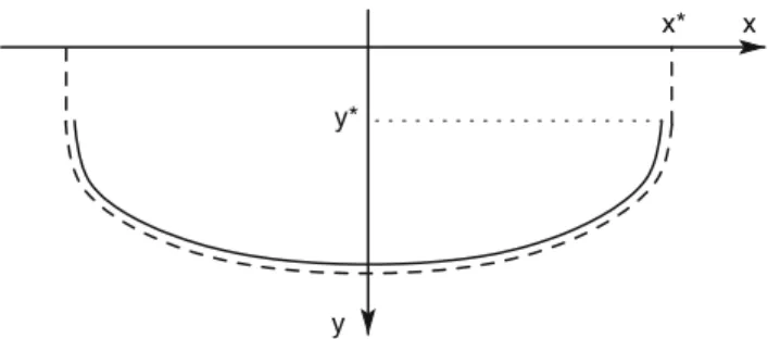
Appendix: Determination of the plug zone depth When the velocity gradient φ tends to zero, the iso-velocity lines going to the free surface tends to the solution for a constant coefficient of friction (Eqs.10and11) (continuous line in Fig.8), when the angle α remains lower thanπ
x
y y*
x*
Fig. 8 Sketch of the constant coefficient of friction solution
(conti-nuous line) and I−dependent coefficient of friction limit solution when the velocity gradient φ tends to zero (dashed line)
The constant friction solution attains α = π
2 at a point
(x∗,y∗)below the free surface for h > Rℓ−1s . This point is attained for s= s∗, with cos(ks∗)= −1/R.
After that, the iso-velocity lines tends to reach the free surface like a straight line normal to it, as sketched in Fig.8 in dashed line.
hplugis obtained by equating the shear force acting on the
limit iso-velocity line with the weight in the z-direction. It writes: s∗ ( 0 (ℓs+ y|cst)2ds+ y∗ ( 0 (ℓs+ y)dy −R s∗ ( 0 y|cstdx ds |cstds= 0, (25)
where the cst-suffix means that we take the constant friction solution. This leads to the solution:
hplug= ℓs R− 1 ⎛ ⎝1 + -1+ R2s∗ 1+ s∗ ⎞ ⎠ . (26)
The half-width of the plug is:
xplug = ℓs ⎛ ⎝R + -1+ R2s∗ 1+ s∗ ⎞ ⎠ 1+ s∗ R2− 1. (27) References
1. Brewster, R., Crest., G.S., Landry, J.W., Levine, A.J.: Plug flow and the breakdown of bagnold scaling in cohesive granular flows. Phys. Rev. E 72, 061301 (2005)
2. Da Cruz, F., Emam, S., Prochnow, M., Roux, J.N., Chevoir, F.: Rheophysics of dense granular materials: discrete simulations of plane shear. Phys. Rev. E 72, 021309 (2005)
3. Daerr, A., Douady, S.: Two types of avalanche behaviour in gra-nular media. Nature 399, 241–243 (1999)
4. de Ryck, A., Ansart., R., Dodds, J.A.: Granular flows down inclined channels with a strain-rate dependent friction coeffi-cient. Part I: non-cohesive materials. Granular Matter (2007).
doi:10.1007/s10035-008-0105-3
5. Forterre, Y., Pouliquen, O.: Long-surface-wave instability in dense granular flows. J. Fluid Mech. 486, 21–50 (2003)
6. Hatano, T., Otsuki, M., Sasa, S.I.: Criticality and sca-ling relations in a sheared granular material. J. Phys. Soc. Jpn. 76(2), 023001 (2007)
7. Jop, P., Forterre, Y., Pouliquen, O.: A constitutive law for dense granular flows. Nature 441, 727–730 (2006)
8. Komatsu, T., Inagaki, S., Nakagawa, N., Nasuno, S.: Creep motion in a granular pile exhibiting steady surface flow. Phys. Rev. Lett. 86(9), 1757–1760 (2001)
9. Pouliquen, O., Renaut, N.: Onset of granular flows on an inclined rough surface: dilatancy effects. J. Phys. II Fr. 6, 923–935 (1996) 10. Rognon, P.G., Roux, J.-N., Wolf, D., Naaïm, M., Chevoir, F.: Rheophysics of cohesive granular materials. Europhys. Lett. 74(4), 644–650 (2006)
11. Rognon, P.: Rheology of cohesive materials—application to dense snow avalanches. Ph.D. Thesis (in french), École Nationale des Ponts et Chaussées (2006)
12. Rumpf, H.: Zur Theorie der Zugfestigkeit von Agglomeraten bei Kraftübertragung an Kontaktpunkten. Chemie Ingenieur Tech-nik 42(8), 538–540 (1970)
13. Wood, D.M.: Soil behaviour and critical state soil mecha-nics. Cambridge University Press, Cambridge (1990)