COMBINATION OF EXPERIMENTAL AND SIMULATED SMALL
SCALE SOLAR AIR-CONDITIONING SYSTEM
Sébastien THOMAS*, Samuel HENNAUT and Philippe ANDRE University of Liège
BEMS team, Building Energy Monitoring and Simulation
Department of Sciences and Environmental Management 185, Avenue de Longwy, 6700 Arlon, Belgium * Corresponding Author, sebastien.thomas@ulg.ac.be
Abstract
It is now clearly assumed that solar assisted air conditioning is able to decrease CO2 production
of building operation. One way to evaluate the energy savings potential is the simulation of air-conditioning systems. On the other hand, it is also crucial to assess system performance by experimentations. The operation of a solar cooling system in its real environment is considered here. The objective is to evaluate if sun radiation in our region (Western Europe – Belgium) in summer 2009 is enough for feeding an adsorption chiller, in other words to find experimentally the solar fraction of a solar air-conditioning system in our region. Residential application suits with equipment available in our laboratory. A combination of experimentation and simulation is used because of the lack of sorption chiller in our laboratory facilities. Hot loops are measured while cold and rejection loops are simulated. Thirty-one days were measured; energy flows analysis on the whole period reveals a theoretical solar fraction of nearly 100% but a real solar fraction of 31%. Issues related to the test implementation are emphasized and explained in this paper.
Keywords: Solar cooling, adsorption, experimentation, simulation 1. Introduction
Solar air-conditioning is a good way to use renewable energy instead of fossil fuels. Currently there are around 300 [1] systems in operation all other the world. That's why a lack of awareness of such
technologies is still encountered. For practical cases, it is generally difficult to evaluate accurately the possible energy savings. It is proposed in this work to assess the potential of solar energy when operating an air-conditioning system to cool a house. The air-conditioning system considered here is a thermally driven adsorption chiller.
A combination of experimental and simulated scheme (figure 1) is proposed because of available equipment in our laboratory. Solar loop containing 14 m² flat plate collectors and two storage tanks (300l and 1000l) are effectively installed in the Jacques Geelen Laboratory located in Arlon (Belgium). On the other hand, the adsorption chiller and the cooling load are simulated.
The objective is to evaluate the solar fraction of this combined experiment-simulation cooling system in real conditions in summer 2009 in our region (South of Belgium). Solar fraction (SF) is defined as follows:
chiller ADS run to required Heat panels solar by provided Heat SF = (equ. 1)
Fig. 1. Solar air conditioning system tested in Jacques Geelen laboratory during summer 2009. The equipment and simulations are discussed in the following paragraph. Firstly, the modelling and simulation of emulated equipment are explained. Secondly, the laboratory facilities are described and finally the computation of results is exposed.
2. Method: Simulation 2.1. Cooling load
The idea is to evaluate the cooling load of an average house in our region in real conditions. It has been decided to simulate a typical house. The selected building is a 145 m² cooled semi detached house. Room surfaces glazing area, internal gains (people, cooking, light, appliances) as well as wall properties are defined in previous studies [2] [3]. The building is modelled in TRNSYS [4]. The selected building’s orientation and roof slope are the same as for the laboratory. In this way we can consider we have the same solar radiation on the roof of the laboratory and on the simulated house. Ventilation air flows are set up according to the Belgian regulation [5], leading to a total volume flow of 180 m³/h (0.89 volume per hour). While cooking an additional flow of 160 m³/h is considered. For both flows, no heat-cool recovery is considered.
Walls constitution can be summarized by U values in W/(m² K) : ground floor Ug=0.48, external wall
Uw=0.38, roof Ur=0.39. Windows selected have a Ug value of 3.4W/(m² K). Double glass has a
U-Value of 3 while frame U-value is 5.68 (85% of window area is glass). The g-value is 0.722. Automatic solar protections are used (55% efficiency).
This residential building suits very well to the cooling load achievable by the installed solar field. Regarding a rough static design method [6] to find the collector area, maximum cooling power should be round about 4 kW (Qcool in equation 2).
COP G Q A cool ⋅ ⋅ =
η
(equ. 2) withA = solar collector area = 14 m²; G = incident radiation = 1000 W; η = collector efficiency = 0.6;
COP = thermal COP of adsorption chiller = 0.5.
The tricky point is to find cooling load of simulated house in real (measured) conditions. It seems that cooling load is correlated with external temperature. In this case, dynamic effects are predominant; therefore the time scale of a day is not short enough. Running building simulation with TRNSYS in summer season (June-September) with Trier (German city 60 km away from Arlon) meteorological data reveals a correlation between whole zones cooling load and external temperature on an hourly basis. It is then possible to find the cooling load of the simulated house in real current conditions. For each hour of the day a different linear correlation is found. Cooling loads lower than 0.5 kW are not taken into account in our analysis because it is assumed as the minimum part load operation of the adsorption chiller. The linear correlation coefficient is presented for each hour on figure 2. Hours with poor coefficient are those with lower cooling load. All correlations have the same kind of linear equation:
Qload [kW] = Text [°C] M + B (equ. 3)
0 10 20 30 40 50 60 70 80 1 3 5 7 9 11 13 15 17 19 21 23 Hour of the day
C o o li n g l o a d [ k W h ] * 0 0.1 0.2 0.3 0.4 0.5 0.6 0.7 0.8 0.9 R ² Cooling load [kWh] Correlation coef
* For period from June to September with Trier TMY2 data
Fig. 2.Correlation coefficient for the cooling load 2.2. Adsorption chiller
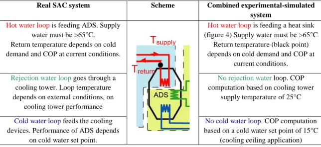
As shown on figure 1, adsorption chiller (ADS) stands at the interface between simulation and experimentation. The only chiller with nearly full available data was adsorption chiller SORTECH ACS 08 [7]. The system is regarded a continuous process. SORTECH ACS 08 real chiller has a nominal cooling power of around 8 kW. For the test, we consider this chiller with half capacity. Hereunder is presented a table with the comparison between a real Solar Air-Conditioning (SAC) system and the work done in this test. COP mentioned in the following paragraphs always refers to thermal COP of adsorption machine.
Table 1. Real SAC system versus Experimental-Simulated.
Real SAC system Scheme Combined experimental-simulated
system Hot water loop is feeding ADS. Supply
water must be >65°C. Return temperature depends on cold demand and COP at current conditions.
Hot water loop is feeding a heat sink (figure 4) Supply water must be >65°C
Return temperature (black point) depends on cold demand and COP at
current conditions.
Rejection water loop goes through a cooling tower. Loop temperature depends on external conditions, on
cooling tower performance
No rejection water loop. COP computation based on cooling tower
supply temperature of 25°C
Cold water loop feeds the cooling devices. Performance of ADS depends
on cold water set point.
No cold water loop. COP computation based on a cold water set point of 15°C
(cooling ceiling application)
The nominal capacity and the COP of the chiller depend only on hot water supply temperature. A polynomial regression based on manufacturer data [7] is entered into the laboratory software. The heat demand related to building cold demand can be computed in real time. Functions computed in real time stand in next table.
Table 2. Functions real time computed
Function Parameter Unit
Chiller COP T supply [-]
Chiller nominal cooling load T supply [kW]
Building cooling load Hour of the day, External t° [kW] Chiller heat demand Building cooling load, Chiller nominal cooling load, COP [kW] T return T supply, Chiller heating load, Cp water, water mass flow [°C] 3. Method: Experimentation
The other part of the system is really effectively installed in the laboratory. It includes a 14m² solar collector field [8], a water storage and a heat sink (figure 3 respectively left – middle - right).
3.1. Solar loop
Solar loop converts solar energy into heat. It contains six flat plate collectors [8] for a total of 14 m², a draining system with pump (Dynasol on figure 3). The collector's orientation is 43° East while slope is 42°. Temperature is measured on the supply and return pipe and a mass flow meter is installed in the circuit. Moreover, a pyranometer stands on the roof near the panels (with the same orientation and slope). It will give the opportunity to compute the collectors yield.
3.2. Storage
Two water storages are considered successively (300liters and 1000liters); heat is provided by solar collectors and removed by hot water loop (containing heat sink). At least two temperatures probes are in each tank. Solar tank are insulated with 5 to 7 centimetres rock wool insulation material. Heat losses are computed based on a model of tank validated with previously run experimentations.
3.3. Heat sink
A heat exchanger coupled with a variable fan speed (figure 4 - right) and a pump is our controllable heat sink. It is directly plugged on the tank and rejects heat outside of the laboratory. A variable speed fan controls the quantity of heat rejected to track the heat consumption of simulated adsorption chiller (T return in table 1 – 2). Pump has an ON-OFF signal depending on temperature available in the tank and on the cooling load (table 2). Temperature and mass flow are measured; heat removed from tank is then computed.
A big issue encountered is a thermosiphon effect during the night. At this moment, pump is off and storage tank contains water at relatively high temperature (generally around 60°C) while external heat sink remains at low temperature (15-20°C). It implies an unwanted fluid circulation which is rejecting heat in the atmosphere. This effect has dramatically decreased the solar fraction of the system. 4. Results
4.1. Energy balance
The objective is to compute a solar fraction (defined in equation 1). Assisted by measurement, this energy balance is computed (obviously, Q balance is theoretically equals to zero):
Q balance = Q from panels - Q tank losses - Q heat sink - Q thermosiphon (equ 4) More info is available, in particular building cooling load and adsorption required energy are
integrated. Finally the available solar energy is also computed. As measurements are done each minute heat flow can be presented with different time scale. On a daily basis, total integrated energy as well as dynamic behaviour are presented. The whole test (31 days) results are also presented.
4.2. Daily results
On a daily basis the results are presented for a typical hot day in August (test with 1000l storage). Figure 4 describes the heat flows through this day. Solar field gives a maximum power of 7 kW.
Q_cold_required is the computed cooling load of the house (limited > 0.5 kW see § 2.1); it is clearly
delayed with respect to the solar radiation, what implies high cooling load in the night when sun is not shining anymore. The maximum cooling load is always (even in other sunny days) under the value of 4 kW designed in §2.1. Q_heat_required is the heat required by simulated Adsorption chiller to satisfy
the cooling load. Q_hot_water is the heat really rejected by heat sink. For the whole test the control of the heat sink is limited; rejected power lower limit is 2.5-3 kW while upper limit is 5 kW. It is
obviously a limitation of the test. Q_thermosiphon is the unwanted heat flow due to thermosiphon explained above; it has a big impact on results (figure 5 and 6). Some typical periods are pointed out on left of the graph. The period when solar radiation is able to satisfy the cooling load is quite short.
Fig. 4. Heat flows during a sunny day
The energy is integrated on the whole day for two hot days in August (figure 5 where first bars are August 7th August and second bars are August 16th). The measured values (mass flow multiplied by temperature gap) are Energy from panels, Energy to heat sink, Energy on panels. The other energy quantities are computed (based on measurements). Theoretical solar fraction is Energy from panels divided by Heating Energy Required, it reaches 50 to 60%. Practically, the solar fraction measured is
Energy to heat sink divided by Heating Energy Required; it is only 20%! Thermosiphon effect and
other losses are explaining this huge shrinkage of solar fraction. Moreover it can be seen that solar panel efficiency (Energy from panels / Energy on panels) is around 50% because of high temperature flow. High daily cooling load are encountered (between 30 and 40 kWh). The variability is high when speaking about cooling load. The hottest summer day attains 53 kWh. Daily solar energy available varies from 1.8 to 7.4 kWh/m². 0 10 20 30 40 50 60 70 80 90 Energy from panels [kWh] Energy to heat sink [kWh] Tank losses [kWh] Thermosiphon losses [kWh] Cooling load (limited > 0.5 kW) [kWh] Heating energy required (limited >0.5 kW) [kWh] Energy on pannels [kWh] E n e rg y [ k W h ]
4.3. Storage strategies
Comparison can be achieved between the use of a 300l and 1000l storage. Larger storage improves system stability from heat sink side and solar loop. ON-OFF cycles of the heat sink do not appear in 1000l test, it implies a better operating condition for adsorption chiller. Starting time is obviously later with 1000l than with 300l. During test, earlier starting point was 9 AM with 300l and 10 AM with 1000l. Latest starting time with 1000l is 11 AM. Simulated house inertia implies a delay in cooling load (in comparison with solar available energy). Using a 1000l or more is not problematic because solar cooling system will be able to start on time to cool the house. Orientation of solar field (South-East) is exhorting early start of the system. From a solar fraction point of view, the different tests with 300l and 1000l storages has achieved the same solar fraction. Without thermosiphon effect, 1000l storage should be able to store enough energy in the day to cool the house during the night while 300l is too small.
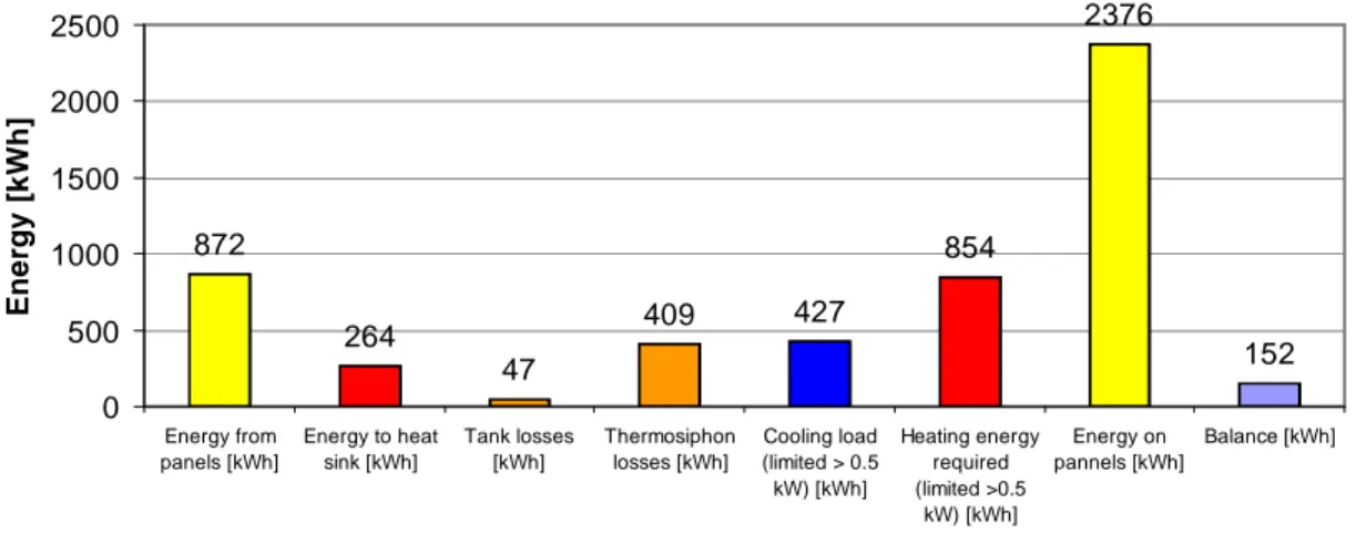
4.4. Whole test results
Nearly each day from end of July to early September were recorded. A total of 31 days test furnishes results about energy quantity (explained in previous paragraph). Moreover the Balance column is added to the bar chart on figure 6. It represents the error on energy balance (equation 4) that is due to losses not taken into account and other error in measurements. Balance error is 17% of the total energy collected by solar field; this high value is really annoying for the overall performance analysis. On this time scale basis the theoretical solar fraction is (872-47)/854 ≈ 97%. For the whole period, it means that sun is nearly enough to operate an adsorption chiller to cool a house. The real achieved solar fraction is 31%. This is partly due to thermosiphon effect. Of course, this time scale analysis assumes all the solar energy coming from solar thermal field can be stored. In our test, it was the case because of thermosiphon effect emptying the storage each day. A 1000l water storage can store one quite sunny day (6 kWh/m² collector) without cooling load (no hot water draw). More than one sunny day without cooling load is rare. So the hypothesis of 100% storage is not so bad for this small scale solar cooling application.
872 264 47 409 427 854 152 2376 0 500 1000 1500 2000 2500 Energy from panels [kWh] Energy to heat sink [kWh] Tank losses [kWh] Thermosiphon losses [kWh] Cooling load (limited > 0.5 kW) [kWh] Heating energy required (limited >0.5 kW) [kWh] Energy on pannels [kWh] Balance [kWh] E n e rg y [ k W h ]
Fig. 6. Energy values for the whole test (31 days)
Solar collector yield on the whole test is lower than in sunny days, it reaches 37% instead of +/- 50%. This is due to high temperature in the storage, sometimes solar radiation cannot reach easily this
temperature in the panels. Thus, there are some periods where the sun is shining but no heat is transferred by solar collectors.
5. Conclusion
A combination of experimental and simulated small scale air-conditioning system was presented in this paper. The idea was to evaluate the system solar fraction in real conditions in our region. The real time coupling between installed solar loop and simulated adsorption chiller works; the heat sink is able to dissipate an energy quantity closed to the amount of energy requested by adsorption chiller to cool a house. Despite the measurement issues and errors, system ran during thirty-one days and gave interesting results. A 31% solar fraction was achieved during the test; this is a very low and not so promising value. However, the potential of solar energy to cool a building is higher. Taking into account energy from panels and tank losses, 95% of cooling load can be satisfied by solar energy via adsorption chiller. Equipment used suits very well to a residential solar cooling application.
Moreover, two water storages were tested, the 1000l tank seems to be enough for this application and avoid ON-OFF cycles of the system which are decreasing COP. The delay between solar available energy and cooling load as well as the building orientation are also supporting this kind of storage. Finally, issues encountered are taken into account to improve experimentations in summer 2010. Same kind of test is run in summer 2010 in the laboratory in Arlon. The balance error of 17% is obviously too high, new measuring devices are installed to measure more accurately the heat flows. Furthermore, thermosiphon dramatically affects the solar fraction; a check valve is installed to avoid this effect. Heat sink power range is boosted by a variable speed pump for this hot water loop.
By running these new tests we hope to find the real possible solar fraction in order to evaluate the profitability of residential solar cooling application in our region.
References
[1] W. Sparber, A. Napolitano (2009). IEA-SHC Task 38. List of existing solar heating and cooling installations. Available online http://iea-shc-task38.org/documents/monitoring2 (last visit: 10 June 2010)
[2] Oscar Ortiz, et al. (2008). Sustainability based on LCM of residential dwellings: A case study in Catalonia, Spain , Building and Environment, vol 44 issue 3, 584-594
[3] Thomas. S (2008) Cooling needs of a Mediterranean house
[4] TRNSYS simulation studio, Version 16.00.0038 Licensed to University of Liège [5] Belgian norm NBN D50-001 (1991) Ventilation systems for housings
[6] Henning, H.-M. (2007). Solar-Assisted Air-Conditioning in Buildings, A Handbook for Planners (Second Revised Edition), Springer-Verlag/Wien.
[7] SorTech AG company (2008) SorTech Adsorptionskältemaschine – Planungsanleitung, version 1.3 [8] DIN CERTO (2008) Annex to Solar Keymark certificate of ESE Eco solar 2.32 flat plate collector.
http://solarkey.dk/solarkeymarkdata/CollectorCertificates/solarkeymarkCollectorCertificates.aspx (last visit 10 June 2010)