Soft-SAFT modeling of vapour liquid equilibria of nitriles and their mixtures

Any correspondence concerning this service should be sent to the repository administrator:

staff-oatao@inp-toulouse.fr

O

pen

A

rchive

T

oulouse

A

rchive

O

uverte (

OATAO

)

OATAO is an open access repository that collects the work of Toulouse researchers and makes it freely available over the web where possible.

This is an author -deposited version published in: http://oatao.univ-toulouse.fr/ Eprints ID: 3515

To link to this article:

DOI:10.1016/j.fluid.2009.12.012

URL:

http://dx.doi.org/10.1016/j.fluid.2009.12.012

Belkadi, Abdelkrim and Hadj-Kali, Mohamed and Llovell, Felix and Gerbaud, Vincent and Vega, Lourdes F. ( 2010) Soft-SAFT modeling of vapour liquid equilibria of nitriles

SOFT-SAFT MODELING OF VAPOR LIQUID

EQUILIBRIA OF NITRILES AND THEIR MIXTURES

A. Belkadi1, M. K. Hadj-Kali1, F. Llovell2,3,§, V. Gerbaud1*, L. F. Vega2,3*

1_{Université de Toulouse, LGC (Laboratoire de Génie Chimique), CNRS, INP, UPS,}

4 allée Emile Monso - BP 84234 - 31432 Toulouse cedex 4 – France

2_{MATGAS Research Center (Carburos Metálicos/Air Products, CSIC, UAB), Campus}

UAB. 08193 Bellaterra, Barcelona Spain

3_{Institut de Ciència de Materials de Barcelona, (ICMAB-CSIC), Consejo Superior de}

Investigaciones Científicas, Campus de la UAB, 08193 Bellaterra, Barcelona, Spain

* _{Corresponding authors: Vincent.Gerbaud@ensiacet.fr, vegal@matgas.com.}

§ _{Present address: Department of Chemical Engineering, Imperial College London, South Kensington}

Abstract

Nitriles are strong polar compounds showing a highly non-ideal behavior, which makes them challenging systems from a modeling point of view; in spite of this, accurate predictions for the vapor-liquid equilibria of these systems are needed, as some of them, like acetonitrile (CH3CN) and propionitrile (C2H5CN), play an important role as organic

solvents in several industrial processes. This work deals with the calculation of the vapor - liquid equilibria (VLE) of nitriles and their mixtures by using the crossover soft-SAFT Equation of State (EoS). Both polar and associating interactions are taken into account in a single association term in the crossover soft-SAFT equation, while the crossover term allows for accurate calculations both far from and close to the critical point. Molecular parameters for acetonitrile, propionitrile and n-butyronitrile (C3H7CN)

are regressed from experimental data. Their transferability is tested by the calculation of the VLE of heavier linear nitriles, namely, valeronitrile (C4H9CN) and hexanonitrile

(C5H11CN), not included in the fitting procedure. Crossover soft-SAFT results are in

excellent agreement with experimental data for the whole range of thermodynamic conditions investigated, proving the robustness of the approach. Parameters transferability has also been used to describe the isomers n-butyronitrile and i-butyronitrile. Finally, the nitriles soft-SAFT model is further tested in VLE calculation of mixtures with benzene, carbon tetrachloride and carbon dioxide, which proved to be satisfactory as well.

1. Introduction

Accurate thermodynamic properties of pure compounds and mixtures, in particular phase equilibrium properties, are needed over a wide range of temperature and pressure for the optimization of existing processes and the design of new processes and/or materials in chemical industry.Nitriles are industrial solvents and good representatives of polar compounds whose phase equilibria is not trivial to model with macroscopic thermodynamic models, due to their non-ideal behavior [1]. Classical cubic equations of state are usually not suitable for the calculation of polar molecules, unless modifications of pure compound attractive term are introduced and complex mixing rules are used [2]. Activity coefficient models handle polar compounds but are valid only at low pressures. Recently, Hadj-Kali et al. [3] used molecular simulation techniques by coupling the Gibbs Ensemble Monte Carlo method with a suitable interaction force field including columbic interaction to model vapor - liquid equilibrium of such molecules; although these molecular simulations provided excellent insights, they required an intensive computational effort compared to the immediate results obtained from equation of state models, making them still inappropriate for routine calculations needed in process design.

Much effort has been devoted in recent years towards the development of molecular-based equations of state (EoS). Their main advantage versus classical methods is that the molecular structure (chain structure, polarity and association) is explicitly built into the equation from its inception, allowing them to accurately predict the behavior of such complex fluids. Among these predictive methods, the Statistical Associating Fluid Theory (SAFT) [4-6] and its more refined versions are becoming a very popular tool in academic and industrial environments due to its success in predicting the behavior of a wide variety of industrial relevant mixtures, for which other equations fail.

This theory has generated a series of different versions of what are now known as SAFT-type equations, all of them based on Wertheim’s first-order thermodynamic perturbation theory (TPT1) [7-10]. The most popular version of this equation was developed by Huang and Radosz [6]. These authors parameterized the equation for several pure fluids and mixtures showing its applicability for real engineering applications from its development. Other recent, more refined, modifications of SAFT include the soft-SAFT equation of Vega and co-workers [11-13], the SAFT-VR equation of Jackson and co-workers [14] and the PC-SAFT equation of Sadowski and co-workers [15]. All SAFT-type equations use Wertheim’s first order perturbation theory for the chain and association term, while they differ mainly in the reference term. A detailed discussion on the success and limitations of SAFT equations, improvements, and applications can be found in three excellent reviews published on the subject [16-18].

In this work we have used the soft-SAFT EoS, developed by Blas and Vega [11] and its crossover extension [19] to test the capability of this equation to accurately describe the phase equilibria of nitriles and their mixtures. Unlike classical equations of state, such as Peng-Robinson (PR) or Soave-Redlich-Kwong (SRK), which require previous knowledge of certain thermodynamic properties for each compound (critical temperature, critical pressure and acentric factor) to model their PVT properties, a molecular based EoS requires to describe the gross chemical structure of molecules in terms of molecular parameters, usually obtained by fitting vapor-liquid equilibrium data. A correlation of these parameters with the molecular weight of the compounds for the same chemical family enables to obtain the PVT data of members of the same homologous series not included in the fitting procedure.

The present paper is organized as follows: a brief background of the crossover soft-SAFT EoS is described next, with particular attention to the crossover treatment which greatly improves the modeling of the critical region. Details on nitriles former published models and the proposed model are provided in the next section. Finally, molecular parameters are regressed for the three lightest nitriles of the linear nitriles family and their transferability is validated for heavier compounds of the same family, in a pure predictive manner. Mixture VLE of nitriles with benzene, carbon tetrachloride and carbon dioxide are also given. Some concluding remarks are provided in the last section.

2. The crossover soft-SAFT equation of state

The general expression for SAFT is given in terms of the residual Helmholtz energy, ares defined as the molar Helmholtz energy of the fluid relative to that of an ideal gas at the same temperature and density. This residual Helmholtz energy can be obtained as the sum of the different microscopic contributions. For the systems investigated in this work, the general expression of the SAFT equation is:

polar assoc chain ref id res _{a a a a a a} a       (1)

where a and aid are the total Helmholtz energy density and the ideal gas Helmholtz energy density at the same temperature and density, respectively. aref is the reference contribution to the Helmholtz energy of the spheres term composing the molecules and it usually includes the attractive and repulsive forces among the spheres forming the chains. achain, the chain contribution term, and aassoc, the association term, both coming from Wertheim’s theory. Finally, apolar takes into account the polar contribution to the

Helmholtz energy. In essence, the total Helmholtz energy in the SAFT approach is the sum of different microscopic contributions, all of which can be taken into account in a systematic manner.

The main difference between the soft-SAFT equation and the original SAFT equation [3-4] is the use of the Lennard–Jones (LJ) intermolecular potential for the reference fluid in the soft-SAFT equation, with dispersive and repulsive forces explicitly considered into the same term, instead of the perturbation scheme based on a hard-sphere reference fluid plus dispersive contributions to it. This difference also appears in the chain and association term, since they both use the radial distribution function of the reference fluid, and it has turned out to be relevant for some applications of the equation [20].

Hence, the reference term in the soft-SAFT EOS is a LJ spherical fluid, which represents the units making up the chains. Following previous work, we have used the accurate EoS of Johnson et al. [21] for this term.

The chain term, achain_{, accounts for the energy of formation of chains from units}

of the reference fluid. This term is obtained by taking the limit of complete bonding in Wertheim’s TPT1, and it is formally identical in all versions of SAFT. The Helmholtz free energy due to the formation of chains from mi spherical segments can be written as:



where ρ is the molecular density of the fluid, T is the temperature and kB is the Boltzmann constant. In the soft-SAFT case, it is applied to tangent LJ spheres of chain length m that are computed following a pair correlation functiong , evaluated at the _LJ

The association term comes from Wertheim’s TPT1 for associating fluids. The Helmholtz energy density change due to association is calculated from the equation:

 

where Mi is the number of associating sites of component i and X the mole fraction of i component i not bonded at site α, which accounts for the contributions of all associating

sites in each species:

 



The term ij is related to the strength of the association bond between site  in molecule i and site  in molecule j, from which two additional molecular parameters,

related to the association, appear: ij _{, the association energy and} i j _{, the}

association volume for each association site and compound.

The number of association sites for each molecule, as well as the allowed interactions among the sites, has to be specified a priori within the SAFT approach. In this work, we consider all association interactions to be equivalent, i.e., all sites have the same values for the ij _and i j _parameters.

The extension of the equation to polar systems is done by adding a new contribution that consists in a perturbed polar term proposed by Gubbins and Twu [22]. For the case of the quadrupole this term is:













































a

a

a

a

1

1

Expressions for

a

a

Since the reference term is written and established for a pure compound (in contrast with the chain, association or polar terms, which are directly applicable to mixtures), the residual Helmholtz energy density of the mixture is approximated by the residual Helmholtz energy density of a pure hypothetical fluid, using the van der Waals one fluid theory. The resulting mixing rules are written as:

2 3 3       











The above equations involve the mole fraction xi and the chain length mi of each of the components of the mixture of chain. The crossed interaction parameters _ij and

ij

2 jj ii ij ij       (9) jj ii ij ij      (10)

where the factors ηij and ξij, that modify the arithmetic and geometric averages between components i and j, are the adjustable size and energy binary parameters of this

equation. Note that ij is (1-kij) in most equations of state. With the expressions in eqs 6-10, the reference term is expressed as a function of the chain molar fractions. The validity of these rules to achieve excellent results has been proved in other works [25-27].

An extension of the original equation includes the addition of a crossover treatment to take into account the contribution of the long-wavelength density fluctuations in the near critical region, the so-called crossover soft-SAFT EoS [19]. Based on White’s work [28], from the Wilson’s renormalization group theory [29], this term is implemented by using recursive relations where the density fluctuations are successively incorporated. The crossover soft-SAFT equation has been used along the present work. The Helmholtz energy density of a system at density  can be described in recursive manner as:

 

_



 

 











_a

_a

_da

a







where an is the Helmholtz energy density and dan the term where long wavelength fluctuations are accounted for in the following way:

 

_{ }

 

where s and l represent the density fluctuations for the short-range and the long-range attraction respectively, and Kn is a coefficient that depends on the temperature and the cut off length:

3 3 2 L T k K _nB n  _ (13)

 

 



 









 

The superindex  refers to both long (l) and short (s) range attraction, respectively, and G is a function that depends on the evaluation of the functiona , calculated as:

 

 





 

 





where m is the chain length (number of LJ segments forming the chain),  is an adjustable parameter,  is the interaction volume with units of energy-volume, and w refers to the range of the attractive potential. The values of  and w for the LJ potential

are found in Llovell et al. [19].

The extension to mixtures is done following the isomorphism assumption, in the same way as Cai and Prausnitz [30]. Following this approach the one-component

density is replaced by the total density of the mixture. In addition, calculations are further simplified by using Kiselev and Friend’s approximation [31], in which chemical potentials are replaced by mole fractions as independent variables. Finally, the mixing rules needed to determine the crossover parameters L and  are defined as in [19]:





For practical applications, the summation in equation 11 is extended to five iterations, because no further changes in the properties are observed [19].

Overall, the soft-SAFT EoS needs a minimum of three pure compound parameters to model any non spherical molecule: m, the chain length, σ the diameter of

the LJ spheres forming the chain, and ε the interaction energy between the spheres. For

associating molecules, the association volume κHB and the association energy εHB of the sites of the molecule should be considered; for polar molecules the polar moment (that can be dipolar, quadrupolar or octopolar, depending on the structure) can be explicitly included. These parameters are treated as adjustable when applying the equation for real fluids, although some clear trends within chemical families have been found. The inclusion of the crossover treatment leads to two additional parameters, the cutoff length L, related to the maximum wavelength fluctuations that are accounted for the

uncorrected free energy, and , the average gradient of the wavelet function, used as an adjustable parameter. Finally, when dealing with non ideal mixtures, binary interaction parameters η and ξ are sometimes required.

3. Results and discussion

3.1. Pure Nitriles modeling

Light nitriles like acetonitrile or acrylonitrile often display peculiar behavior because of the short radical bonded to the –CN group, which dominates the interactions. In the modified UNIFAC group contribution method, they are indeed considered as two single groups while other nitriles can be constructed from -CHx and -CH2CN groups

[32].

In the comprehensive work of Spuhl et al. [33], acetonitrile (ACN) was modeled by three different schemes: the first considered ACN as a chain of hard spheres, the second as an associative molecule with one associating site on the nitrile contribution CN, and the third one took into account the dipolar moment of the ACN. Results showed that the third scheme performs the best, the associative model giving very similar results. Earlier, Jackowski’s experimental NMR studies of the propionitrile [34] lead to the presumption that self association interactions must be considered in these systems. As the soft-SAFT formalism explicitly takes into account such self association, it is naturally suited, in principle, for the self-associating nitriles.

In this work we have tried to combine simplicity with accuracy in order to obtain high quality results. The soft-SAFT model proposed here describes all nitriles as chains with a single association site located on the CN group. The dipolar moment is not explicitly considered and its effect is implicitly taken into account in the association scheme, as previously done with other similar systems, including water [20, 35]. All parameter values are obtained by fitting to saturated liquid density (ρliq) and vapor pressure (Psat) data, taken from the Design Institute for Physical Properties (DIPPR) [36] available in Simulis®Thermodynamics component (http://www.prosim.net/) for

each molecule by minimization the following objective function called relative average deviation: 2 1 exp exp 1

_

where Y represents the property data used for the regression, namely ρliq and Psat .

The first three linear nitriles (CH3CN, C2H5CN and C3H7CN) are used as

reference molecules for the optimization of the soft-SAFT EoS molecular parameters (m, σ and ε) by fitting the VLE data summarized in table 1. The (εHB and κHB) association parameters values were fitted differently for acetonitrile and other nitriles. We have found that acetonitrile requires a larger association volume than other nitriles, a fact also observed for the case of methanol in the alkanols family [37].

From the observations of Huang and Radosz [5] about the relation between the association strength εHB and volume κHB value, we can classify nitriles as an associating fluid stronger than alkanols but with a considerable smaller association volume [37], hinting at the fact that associated nitriles may interact at distances smaller than H-bonds found in alkanols (typically 2.8 Ǻ). Belkadi et al. [38] observed the same trend for the NO2/N2O4 reacting system modeling. The different values of the associating parameters

for each case are shown in table 2 for comparison. Since the length of the chain should not affect the strength of the association bonds, except for very short molecules, the parameters of the association sites are set at constant values for all other heavier nitriles starting with propionitrile.

As mentioned in the previous section, a crossover treatment is included to improve the description of the critical region. The crossover approach requires the

adjustment of two additional parameters, the cut-off length L, and . Llovell et al. [19] applied the crossover soft-SAFT to linear alkanes treating both L and  as adjustable parameters. These authors tested the accuracy of the crossover soft-SAFT equation by comparison with molecular simulations of LJ chains and did several studies about the influence of both L and  in predicting the phase envelope when compared to

simulation data. The model was then applied to experimental systems of chainlike molecules, the n-alkanes series, providing a set of transferable parameters equally

accurate far from and close to the critical region. The same procedure was used for studying the n-alkanol series [37], and this is the approach followed here.

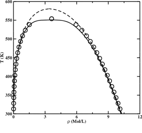
The soft-SAFT parameters obtained in this work are presented in Table 1. The DIPPR vapor pressure and temperature-density diagrams for the first three members of the family are depicted along with the soft-SAFT model with and without crossover in Figure 1. Parameter without crossover for acetonitrile come from Belkadi et al, [41].

The relative average deviation on density and vapor pressure over the entire range is around 6% for calculations without crossover and drops below 1% and 4% range respectively for calculations with crossover. Figure 1 shows that the fitting for the calculations without crossover (dotted lines) is indeed excellent, except near the critical point. This is expected since in that case density fluctuations occurring near the critical region are not explicitly expressed. As shown in these figures the crossover treatment (solid lines), brings remarkable agreement with the experimental data near to and also far away from the critical point.

An advantage of having parameters with physical meaning as in SAFT equations is that their physical trend can be investigated within the same chemical family [13, 39-40]. Therefore, as in previous works [35,37], the three molecular parameters m, mσ3 and

mε and the crossover parameters L and  are linearly correlated (correlation coefficient

higher than 0.99) with the molecular weight MW of the first three members of the n-nitriles: 1083 . 1 0083 . 0   M_W m (21) 878 . 13 1143 . 2 3 _{ } w M m (22) 53 . 263 025 . 3 /k_B  M_W  m (23) 5491 . 8 0603 . 0   M_W m (24) 2904 . 1 0127 . 0 /  M_W  mL  (25)

Units of σ and ε/kB are Å and K, respectively.

The first three correlations were already proposed by Belkadi et al [41] and kept valid. The molecular parameters obtained in this work show the expected trends corresponding to their physical meaning: the value of LJ diameter  obtained for the nitriles series is higher than the corresponding one obtained for alkanols [37] for the same carbon number (indeed the –CN group with a mean C-N bond length of 1.136Å [42] occupies a larger volume than the –OH group with a mean O-H bond length around 0.97Å [43]). Moreover, the energy parameter, ε is slightly greater for nitriles than for the alkanols series [37]. The segment number m is lower than those of the alkanols. Since the length of the chain should not affect the strength of the association bonds, except for very short molecules, the parameters of the association sites are set at constant values, except for those of acetonitrile.

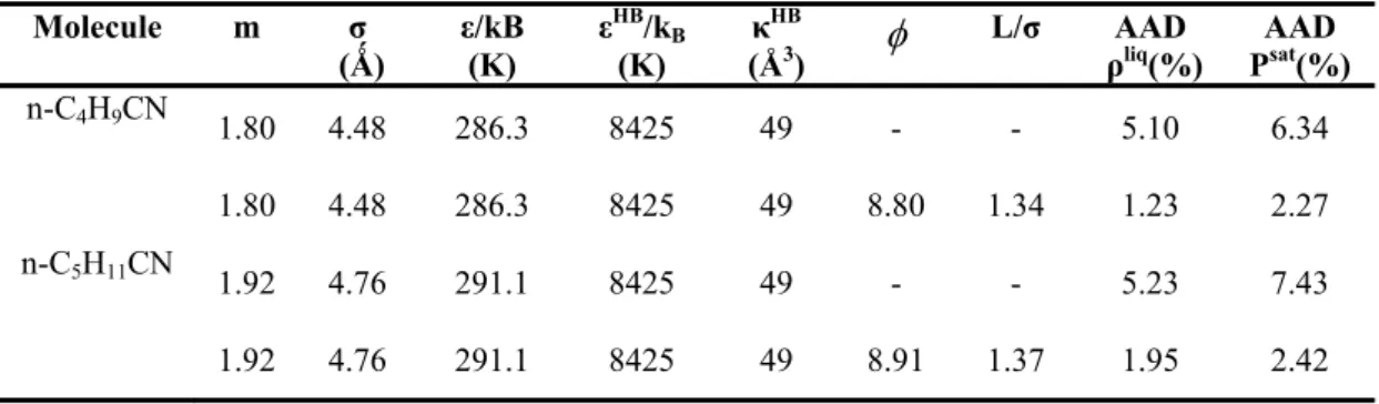
Using the parameter correlations (Eqns. 21- 25), without any further fitting on additional experimental data, VLE properties of heavier linear nitriles of the same family (valeronitrile (C4H9CN) and hexanonitrile (C5H11CN)) are predicted using the

soft-SAFT equation with and without crossover (Table 3), calculations without crossover are taken from ref [41]. The maximum absolute average deviation to density

is obtained for hexanonitrile (0.88%) with an absolute average deviation to the vapor pressure near 3% for both molecules leading to a very good agreement comparing to the DIPPR data as highlighted in Figure 2. The overall agreement with DIPPR data is very good using the original soft-SAFT equation (dashed line), while results in the critical region are improved with the crossover term (solid line), proving the transferability of the parameters used for these predictions.

Finally, soft-SAFT is also able to provide results for isomers; we have investigated the performance for normal and iso butyronitrile.

Results of the fitting show that m and σ parameters (Table 4), that are related to the spatial description of the molecule, are slightly different and in a meaningful way regarding their tridimensional configuration difference: the m value is smaller for the smaller iso-butyronitrile but the σ value is larger as expected because iso-butyronitrile is bulkier. The dispersive energy and the association parameters are kept to be the same than those of n-butyronitrile for both isomers, as the difference between the isomers stands for the structural organization, already taken into account by m and σ.

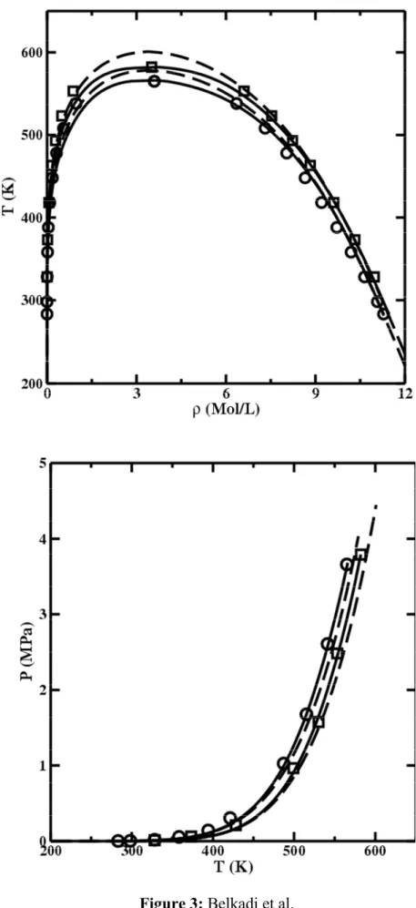
Again, DIPPR data vapor pressure and density diagrams (Figure 3) are well fitted by the soft-SAFT equation without crossover and better with crossover in the critical region. Notice that the critical temperature of iso-butyronitrile is higher than the n-butyronitrile, and the critical pressure is lower. This observation is expected since that the iso-butyronitrile is bulkier than n-butyronitrile.

3.2. Mixtures of nitriles with benzene, carbon tetrachloride and carbon dioxide.

We present here the performance of the crossover-soft-SAFT equation for some mixtures of acetonitrile with benzene (C6H6), carbon tetrachloride (CCl4) and carbon

molecular parameters for each component participating in them are needed. For the three components mixed with acetonitrile we use the parameters already available in the literature, or we fitted them if needed.

The benzene parameters used here, which explicitly include the quadrupole, are taken from the most recent work of Vega et al. [20]. They are used here in a transferable manner and their values are provided in Table 5 for completeness.

Carbon tetrachloride has been modeled in this work as a homonuclear chainlike molecule of m Lennard-Jones segments with equal diameter , and the same dispersive energy ε, bonded tangentially to form the chain. This is exactly the same approach used for n-alkanes and prefluoroalkanes in previous works [19, 27,44] These three molecular parameters plus the crossover parameters L and  are listed in the Table 5. Figure 4 depicts the soft-SAFT coexistence curve for carbon tetrachloride with and without the crossover compared to the DIPPR data. As expected the crossover treatment gives the best results with a relative average deviation around 1% according to Table 5.

The carbon dioxide model, explicitly taking into account the quadrupolar interactions, was taken from the work of Belkadi et al. [38]. The molecular parameters are used here in a transferable manner and their values are also provided in Table 5 for completeness.

Once the molecular parameters of the pure components are available, soft-SAFT can be used to study the behavior of their mixtures. Predictions of the mixtures VLE by using the crossover soft-SAFT equation without any binary interaction parameters were first attempted. Results are displayed in Figures 5 to 9 (see the dashed lines), showing that it is not possible to give an accurate description of the experimental data just from pure component parameters. In particular, the azeotrope point is not predicted for the

mixtures acetonitrile – benzene and acetonitrile – carbon tetrachloride. Hence, one or two binary parameters are needed to accurately describe the mixture behavior.

The use of one or two binary interaction parameters for mixtures involving compounds for which SAFT models are accurate is common, as it takes into account the differences in the size of the two molecules or in their energy of interaction. This is due to the fact that the equation uses the van der Waals one-fluid theory for the mixture, an approximation by which the mixture is considered to be composed of molecules of average size and energy between those of the two components. This is also frequently encountered when modeling mixtures with other popular thermodynamic approaches, either cubic equation of state or activity coefficient models.

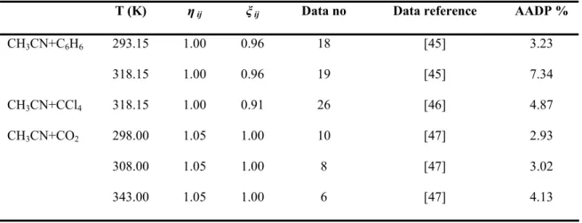
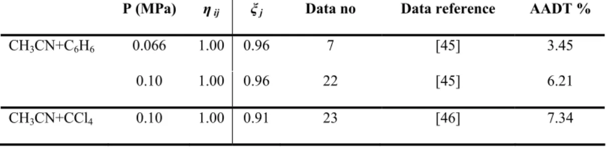
Therefore, the acetonitrile mixtures were modeled with a unique energy binary parameter, introduced by fitting the experimental isotherms data to the percentage average relative deviation on pressure and temperature. Calculations are presented in the Table 6 for the isotherms and Table 7 for isobars. The absolute average deviation from the calculated pressure and temperature is obtained from the Eq. (26):

2 1 exp exp 100



100



















_T

T

T

N

AADT

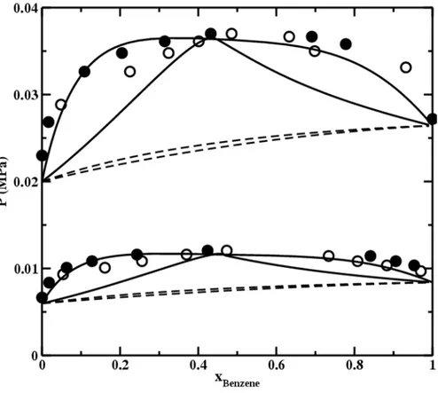
Figure 5 shows a pressure-composition diagram of the benzene - acetonitrile mixture at 293.15K and 318.15K with experimental information taken from the DECHEMA data base [45]; the full lines represent the crossover soft-SAFT calculations with and without binary parameter. The value of the binary parameter ξ = 0.96 is

enough to give quantitative agreement for the whole composition range with AADP around 7%. The azeotrope composition and temperature are well reproduced.

Predictions by using the crossover soft-SAFT equation with the same binary parameter value are done for the benzene - acetonitrile isobars at 0.066 MPa and 0.1MPa with experimental data taken from DECHEMA data base [45]. Results are shown in Figure 6 and good agreement is obtained with a moderate error (see Table 6). The use of the original soft-SAFT equation without crossover (not shown) gives similar results. This is expected since at these conditions the mixture is far away from the critical temperature and pressure of both benzene and acetonitrile.

A second mixture is considered, namely, the tetrachloromethane – acetonitrile mixture. The use of a binary parameter, ξ = 0.91, enables to describe both isotherms at 318.15K (Figure 7) and isobar at 0.1MPa (Figure 8). The relative average deviation is kept below 7% (Table 6 and Table 7). The experimental data are taken from [46]

The last example is the test of the acetonitrile parameters for its mixture with the carbon dioxide. Results of the isotherms at four temperatures are given in Figure 9 with the use of the binary parameter η = 1.05, while keeping ξ = 1. The agreement with the experimental data [47] is good. The choice of size binary parameter η, is the most appropriate for this mixture. We can obtain good results by using the energy binary parameter ξ but its value is then greater than unity. That would differentiate from previous works [35,37] for CO2 in mixtures calculations where when used, the

energy binary parameter ξ was always ξ<1, and with η>1.

4. Conclusions

A molecular model for the n-nitrile chemical family with the soft-SAFT approach was developed. Nitriles were modeled as LJ chains with one associating site mimicking the strong interactions of the –CN group, taking into account in an effective manner the

polarity of the molecules. Once molecular parameters for the first members of the family were obtained by fitting to available VLE equilibrium data, a correlation of these parameters with the molecular weight of the compounds was proposed, used in a predictive manner for heavier members of the family.

The soft-SAFT equation showed its capability to model DIPPR density and vapor pressure data with small discrepancies near the critical region when the original equation was used, while equally accurate results were obtained far from and close to the critical point when the crossover term was taken into account.

The heavier nitriles prediction using the linear correlations were successful, highlighting the reliability of the model. Besides, soft-SAFT was able to make distinction between normal and iso butyronitrile isomers when the appropriate chain length and segment molecular parameters were used.

Finally mixture calculations with benzene, carbon tetrachloride and carbon dioxide showed excellent results compared to experimental isotherms and isobars, with the help of a single temperature-independent binary parameter. For the benzene – acetonitrile mixture, the predictive capacity using a binary parameter regressed on isotherms was shown.

5. ACKNOWLEDGEMENTS

A. Belkadi acknowledges the Ministère de l’Enseignement Supérieur et de la Recherche de France (MESR) for its grants. This research has been possible due to the financial support received from the Spanish Government (project CTQ2008-05375/PPQ), and from the Generalitat de Catalunya (2009SGR-666 and project ITT2005-6/10.05) and from the Région Midi Pyrénées, programme CTP 2005 Région N° 05018784.

List of symbols

AADP Absolute average deviation from the pressure AADT Absolute average deviation from the temperature

a Helmholtz energy density (mol/L) and vdW attractive parameter

g radial distribution function

kB Boltzmann constant (J/K)

L cutoff length in the crossover soft-SAFT equation (m)

m chain length parameter for the soft-SAFT equation

Navog Avogadro’s Number

Np Number of experimental points

P pressure (bar)

Q quadrupolar moment

T absolute temperature (K)

w range of the attractive potential

x integral variable, molar composition

X fraction of not bonded molecules y molar composition

Greek letters

μ chemical potential

 phase density (mol/L)

 crossover constant

 density fluctuation for the short-range and the long-range attraction.

α associating site, interaction volume in the crossover term

 associating site

 mixture binary interaction parameter

 segment diameter parameter for the soft-SAFT equation  dispersive energy parameter for the soft-SAFT equation υ stoechiometric coefficient

κHB volume of association parameter for the soft-SAFT equation

HB _{energy of association parameter for the soft-SAFT equation}

∆ related to the strength of the association interaction

Subscripts 0 zero-order variation c critical i constituent reference max maximum min minimum n nth-order variation r reduced Superscripts s short-range attraction l long-range attraction

 short or long-range attraction

assoc association cal calculated chain chain exp experimental id ideal LJ Lennard-Jones polar polar qq quadrupolar ref reference

6. References

[1] J. Vidal, Thermodynamics: Applications in Chemical Engineering and the Petroleum Industry, Editions Technip, 2003, ISBN2710808005.

[2] J.O. Valderrama, IECR, 42 (2003) 1603-1618.

[3] M.K. Hadj-Kali, V. Gerbaud, X. Joulia, C. Dufaure-Lacaze, C. Mijoule, P. Ungerer, J. Molec. Mod. 14(7) (2008) 571-580.

[4] W.G. Chapman, G. Jackson, K.E. Gubbins, Mol. Phys. 65 (1988) 1057-1079.

[5] W.G. Chapman, K.E. Gubbins, G. Jackson, M. Radosz, Ind. Eng. Chem. Res. 29 (1990), 1709-1721.

[6] S.H. Huang, M. Radosz, Ind. Eng. Chem. Res. 29 (1990) 2284-2294. [7] M.S. Wertheim, J. Stat. Phys. 35 (1-2) (1984) 19-34.

[8] M.S. Wertheim, J. Stat. Phys. 35 (1-2) (1984) 35-47. [9] M.S. Wertheim, J. Stat. Phys. 42 (3-4) (1986) 459-476. [10] M.S. Wertheim, J. Stat. Phys. 42 (3-4) (1986) 477-492. [11] F.J. Blas, L.F. Vega, Molec. Phys. 92 (1997) 135-150.

[12] F.J. Blas, L.F. Vega, Ind. Eng. Chem. Res. 37 (1998) 660-674. [13] J.C Pamies,. L.F. Vega, Ind. Eng. Chem. Res. 40 (2001) 2532-2543.

[14] A.Gil-Villegas, A. Galindo, P.J. Whitehand, S.J. Mills, G. Jackson, J. Chem. Phys. 106 (1997) 4168-4186.

[15] J. Gross, G. Sadowski, Ind. Eng. Chem. Res. 40 (2001) 1244-1260. [16] E.A. Müller, K.E. Gubbins, Ind. Eng. Chem. Res. 40 (2001) 2193-2211. [17] I.G. Economou, Ind. Eng. Chem. Res. 41 (2002) 953-962.

[18]S. P. Tan, H. Adidharma, M. Radosz, Ind. Eng. Chem. Res. 47 (2008) 8063-8082. [19] F. Llovell, J.C. Pàmies, L.F. Vega, Journal of Chemical Physics. 121 (21) (2004), 10715-10724.

[21] K. Johnson, J.A. Zollweg, K.E. Gubbins, Molec. Phys. 78 (1993) 591-618. [22] K.E. Gubbins, C.H. Twu, Chemical Engineering Science. 33 (7) (1978) 863-878. [23] W. Cong, Y. Li, J. Lu, Fluid Phase Equilibria. 124 (1-2) (1996) 55-65.

[24] J.C. Liu, J.F. Lu, Y.G. Li, Fluid Phase Equilibria. 142 (1-2) (1998) 67-82.

[25] L.J. Florusse, J.C. Pàmies, L.F. Vega, C.J. Peters, H. Meijer, AIChE J. 49(12) (2003) 3260-3269.

[26] A.M.A. Dias, J.C. Pàmies, I.M. Marrucho, J.A.P. Coutinho, L.F. Vega, Journal of Physical Chemistry B. 118 (2004) 1450-1457.

[27]J. S. Andreu and L. F. Vega, Journal Of Physical Chemistry B. 112 (2008) 15398-15406

[28] A. White, Fluid Phase Equilibria. 75 (1992) 53-64. [29] K.G. Wilson, Phy. Rev. B. 4 (1971) 3174-3183.

[30] J. Cai, J. M. Prausnitz, Fluid Phase Equilibria. 219 (2004) 205-217. [31] S. Kiselev and D. Friend, Fluid Phase Equilibria. 162 (1999) 51-82.

[32] B.L. Larsen, P. Rasmussen, A. Fredenslund, Ind. Eng. Chem. Res., 26 (1987) 2274-2286

[33] O. Spuhl, S. Herzog, J. Gross, I. Smirnova, and W. Arlt. Ind. Eng. Chem. Res. 43 (2004) 4457-4464

[34] K. Jackowski and E. Wielogorska,. Journal of Molecular Structure. 355 (1995) 287-290.

[35] N. Pedrosa, J. C. Pàmies, J. A. P. Coutinho, I. M. Marrucho, and L. F. Vega, Ind. Eng. Chem. Res. (2005) 44 7027-7037

[36] DIPPR (Design Institute for Physical Property Data) from Simulis® Thermodynamics.

[37] F. Llovell, L.F. Vega, J. Phys. Chem. B. 121 (110) (2006) 1350-1362.

[38] A.Belkadi, F. Llovell, V. Gerbaud, L.F. Vega, Fluid Phase Equilibria. 266 (2008) 154-163.

[39] D. NguyenHuynh , A. Falaix , J.P. Passarello , P. Tobaly , J.C. de Hemptinne Fluid Phase Equilibria. 264 (2008) 184–200.

[40] D. NguyenHuynh, J.P. Passarello, P. Tobaly, J.C. de Hemptinne, Fluid Phase Equilibria 264 (2008) 62–75.

[41] A. Belkadi, V. Gerbaud, M.K. Hadj-Kali, X. Joulia, L.F. Vega, F. Llovell Computer Aided Chemical Engineering. 25(2008) 739-744.

[42] F.H. Allen, O. Kennard, D.G. Watson, A. Brammer, A.G. Orpen, J. Chem. Soc. Perkin Trans. II 1987, S1-S19.

[43] CRC Handbook of chemistry and physics, 89th _{edition. D.R. Lide editor in chief.}

Taylor and Francis eds. Section 9, 2736 pages. ISBN: 142006679X (2009), 9.1- 9.29. Available at http://www.hbcpnetbase.com/.

[44] J.C. Pàmies, L.F. Vega, Molecular Physics. (2002) 100(15) 2519-2529.

[45] J. Gmehling, U. Onken, W. Arlt, Vapor- Liquid Equilibrium Data Collection, Aromatic Hydrocarbons, DECHEMA Chemistry Data Ser., 1980, Vol. I, Part 7, DECHEMA, Frankfurt am Main, Germany.

[46] J. Gmehling, U. Onken, W. Arlt, Vapor Liquid Equilibrium Data Collection, Halogen, Nitrogen, Sulfur and other Compunds, DECHEMA Chemistry Data Ser., 1984, Vol. I, Part 8, DECHEMA, Frankfurt am Main, Germany.

List of captions

Table 1 Original and crossover soft-SAFT optimized parameters for light nitriles (C1 to

C3).

(*) from [41]

Table 2 Comparison of soft-SAFT association parameters for alkanols, nitriles and NO2

Molecule m σ (Ǻ) ε/kB (K) εHB_/k B (K) κHB

(Å3₎  L/σ AAD _ρliq_{(%) P}AAD sat_(%)

CH3CN * 1.45 3.70 268.0 8425 69 - - 5.10 7.24 1.45 3.70 268.0 8425 69 8.47 1.25 0.70 2.83 C2H5CN 1.57 3.98 274.0 8425 49 - - 6.13 5.51 1.57 3.98 274.0 8425 49 8.57 1.27 0.42 2.73 C3H7CN 1.66 4.25 280.0 8425 49 - - 4.54 6.50 1.66 4.25 280.0 8425 49 8.75 1.28 0.95 3.92 molecule εHB_/k B (K) κ HB (Å3₎ Reference

n-alkanols (except methanol) 3600 2300 [37]

acetonitrile other n-nitriles 8425 8425 69 49 This work NO2 – N2O4 6681 1 [38]

Table 3 Original and Crossover soft-SAFT parameters for valeronitrile and hexanonitrile obtained from the correlations. See text for details.

Table 4 Original and Crossover soft-SAFT optimized parameters for normal and iso

butyronitrile.

Table 5 soft-SAFT optimized parameters for benzene from [20], carbon tetrachloride

(this work) and carbon dioxide from [38]. Molecule m σ (Ǻ) ε/kB (K) ε HB_/k B (K) κ HB

(Å3₎  L/σ AAD _ρliq_{(%) P}AAD sat_(%)

n-C4H9CN _{1.80 4.48 286.3 8425 49 - - 5.10 6.34} 1.80 4.48 286.3 8425 49 8.80 1.34 1.23 2.27 n-C5H11CN _{1.92 4.76 291.1 8425 49 - - 5.23 7.43} 1.92 4.76 291.1 8425 49 8.91 1.37 1.95 2.42 molecule m σ (Ǻ) ε/kB (K) ε HB_/k B (K) κ HB

(Å3₎  L/σ AAD _ρliq_{(%) P}AAD sat_(%)

n-C3H7CN 1.66 4.25 280.0 8425 49 - - 4.54 6.50 1.66 4.25 280.0 8425 49 8.75 1.28 0.95 3.92 i-C3H7CN 1.59 4.44 280.0 8425 49 - - 5.28 7.23 1.59 4.44 280.0 8425 49 8.52 1.31 1.05 2.45 Molecule Trange (K) m σ (Ǻ) ε/kB (K) Q

(C.m2₎  L/σ AAD _ρliq_{(%) P}AAD sat_(%)

C6H6(*) 273.0-560.0 2.343 3.754 304.7 -5. 10-40 7.20 1.195 3.34 3.05 C6H6(*) 273.0-560.0 2.333 3.754 299.3 -5. 10-40 - - 1.53 1.05 CO2(+) 220.0-290.0 1.606 3.174 158.5 4.4 10-40 5.70 1.130 0.55 0.82 CO2(+) 220.0-290.0 1.606 3.174 158.5 4.4 10-40 - - 3.54 3.86 CCl4(X) 280.0-600.0 2.225 3.933 308.1 - 6.96 1.200 1.10 0.85 CCl4(X) 280.0-600.0 2.225 3.933 308.1 - - - 4.10 3.85

(*) from [20] (+) from [38] (X) This work

Table 6 Relative average deviation of the calculated pressure for isotherms.

T (K) η ij ξ ij Data no Data reference AADP %

CH3CN+C6H6 293.15 1.00 0.96 18 [45] 3.23 318.15 1.00 0.96 19 [45] 7.34 CH3CN+CCl4 318.15 1.00 0.91 26 [46] 4.87 CH3CN+CO2 298.00 1.05 1.00 10 [47] 2.93 308.00 1.05 1.00 8 [47] 3.02 343.00 1.05 1.00 6 [47] 4.13

Table 7 Relative average deviation of the calculated temperature for isobars.

P (MPa) η ij ξ j Data no Data reference AADT %

CH3CN+C6H6 0.066 1.00 0.96 7 [45] 3.45

0.10 1.00 0.96 22 [45] 6.21

Figure 1 Experimental vapor-liquid equilibrium diagram for acetonitrile [circle], propiontitrile [square] and butyronitrile [cross] with calculation by using the original soft-SAFT (dashed line) and the crossover soft-SAFT (solid line). NIST experimental data are taken from [36]. (a) temperature – density diagram, (b) temperature – vapor pressure diagram. Calculations for acetonitrile without crossover from ref [41].

Figure 2 Experimental vapor-liquid equilibrium diagram for valeronitrile [triangle up]

and hexanonitrile [triangle down] with calculation by using the original soft-SAFT (dashed line) and the crossover soft-SAFT (solid line). NIST experimental data are taken from [36]. (a) temperature – density diagram, (b) temperature – vapor pressure diagram. Calculations for acetonitrile without crossover from ref [41].

Figure 3 Experimental vapor-liquid equilibrium diagram for iso-butyronitrile

[rectangle] and n-butyronitrile [circle] with calculation by using the original soft-SAFT (dashed line) and the crossover soft-SAFT (solid line). NIST experimental data are taken from [36]. (a) temperature-density diagram, (b) temperature- pressure diagram.

Figure 4 Experimental vapor-liquid equilibrium diagram for carbon tetrachloride

[circle] with calculation by using the original soft-SAFT (dashed line) and the crossover soft-SAFT (solid line). NIST experimental data are taken from [36]. (a) temperature - density diagram, (b) temperature- pressure diagram.

Figure 5 Pressure – benzene molar fraction diagram of the acetonitrile + benzene

mixture at 293.15K (square) and 318.15K (circle) are compared with crossover soft-SAFT calculations with a binary parameter used ξ=0.96 (solid line) and without (dashed line). Experimental data from [45].

Figure 6 Temperature – benzene molar fraction diagram of the acetonitrile + benzene

with a binary parameter used ξ=0.96 (solid line) and without (dashed line). Experimental data from [45].

Figure 7 Pressure – tetrachloromethane molar fraction diagram of the acetonitrile +

tetrachloromethane mixture at 318.15K (circle) are compared with crossover soft-SAFT calculations with a binary parameter used ξ=0.91 (solid line) and without (dashed line). Experimental data from [46].

Figure 8 Temperature – tetrachloromethane molar fraction diagram of the acetonitrile +

tetrachloromethane mixture at 0.1MPa are compared with crossover soft-SAFT predictions with a binary parameter used ξ=0.91 (solid line) and without (dashed line). Experimental data from [46].

Figure 9 Pressure – carbon dioxide molar fraction diagram of the acetonitrile + carbon

dioxide mixture at 298.00K (circle), 308.00K (square) and 343.00K (triangle up) are calculations with crossover soft-SAFT predictions with a binary parameter used η=1.05 (solid line) and without (dashed line). Experimental data from [47].

Figure 5: Belkadi et al.

Figure 6: Belkadi et al.

Figure 7: Belkadi et al.

Figure 8: Belkadi et al.