HAL Id: lirmm-00269510
https://hal-lirmm.ccsd.cnrs.fr/lirmm-00269510
Submitted on 6 Jul 2016
HAL is a multi-disciplinary open access
archive for the deposit and dissemination of
sci-entific research documents, whether they are
pub-lished or not. The documents may come from
teaching and research institutions in France or
abroad, or from public or private research centers.
L’archive ouverte pluridisciplinaire HAL, est
destinée au dépôt et à la diffusion de documents
scientifiques de niveau recherche, publiés ou non,
émanant des établissements d’enseignement et de
recherche français ou étrangers, des laboratoires
publics ou privés.
Experimental Dynamic Identification of a Fully Parallel
Robot
Oscar Andrès Vivas, Philippe Poignet, Frédéric Marquet, François Pierrot,
Maxime Gautier
To cite this version:
Oscar Andrès Vivas, Philippe Poignet, Frédéric Marquet, François Pierrot, Maxime Gautier.
Experi-mental Dynamic Identification of a Fully Parallel Robot. ICRA: International Conference on Robotics
and Automation, Sep 2003, Taipei, Taiwan. pp.3278-3284. �lirmm-00269510�
Experimental dynamic identification of a fully parallel robot
Andrès Vivas* Philippe Poignet* Frédéric Marquet* François Pierrot* Maxime Gautier§
*Laboratoire d’Informatique, Robotique et Microélectronique de Montpellier - UMR CNRS 5506, 161 Rue Ada, 34392 Montpellier cedex 5, France
§Institut de Recherche en Communication et Cybernétique de Nantes, UMR CNRS 6597, 1 rue de la Noë, 44321 Nantes cedex 03, France
{vivas, poignet}@lirmm.fr
Abstract - This paper deals with the experimental identification of the dynamic parameters of parallel machines. The dynamic parameters are estimated by using the weighted least squares solution of an over determined linear system obtained from the sampling of the dynamic model along a closed loop exciting trajectory. Experimental results are exhibited for the H4 robot, a fully parallel structure providing 3 degrees of freedom (dof) in translation and 1 dof in rotation. A comparative study is performed depending on the available measurements i.e. different sensor locations (motor, end effector).
1. INTRODUCTION
After the works in parallel mechanisms introduced by Gough [1] or Steward [2], Clavel [3] proposed the Delta structure, a parallel robot dedicated to high-speed applications. In the same way, the “hexapod” [4], [5] has been used intensively in industry. This is due to the exceptional simplicity of the Delta 3-dof solution and the enormous research effort dedicated to the “hexapod”. Many alternate designs have been proposed like the HexaM [6], which is an evolution of the Hexa robot [7]. For most pick-and-place applications, at least four dof are required (3 translations and 1 rotation to arrange the carried object in its final location). For the Delta robot, this is achieved thanks to an additional link between the base and the gripper, but it seems not to be as efficient as a parallel arrangement. On the other hand, 6-dof fully-parallel machines currently used in machining suffer from their complexity (they need at least 6 motors while the cutting process requires only 5 controlled axis plus the spindle rotation) and from their limited tilting angle. As an intermediate solution to these drawbacks, a 4-dof parallel mechanism – the H4 robot - have been proposed [8], [9]. Fig. 1 shows a photography of the H4 parallel robot. This machine is based on 4 independent active chains between the base and the nacelle; each chain is actuated by a brushless direct drive motor fixed on the base and equipped with an incremental position encoder. Thanks to its design, the mechanism is able to provide high performances. In order to achieve high speed and acceleration for pick-and-place applications or precise motion in machining tasks, an accurate dynamic modeling is required to increase the quality of their simulation in order to improve their design and to compute advanced model based robust controllers such as moving horizon control schemes. However the first difficulty is to estimate the physical parameters (mass, inertia and
frictions), especially when the only available measurements are given by the incremental sensors located on the actuators.
Therefore, in this paper, we focus on the estimation of the dynamic parameters of the rigid multi body model. The parameters are estimated by a classical technique of weighted least squares [11], [14]. We mainly discuss two identification results depending on the available measurements. We compare the influence of the sensor locations on the estimation results of physical parameters: i) first, the nacelle acceleration is estimated through the computation of the kinematic model and its derivative ii) secondly, additional sensors (rotation and 3-axis acceleration sensors) located on the end effector provide further measurements.
The paper is organized as follows : Section 2 is dedicated to the geometric, kinematic and dynamic modelling. Section 3 recalls the basis of the identification method. Section 4 exhibits and discuss experimental identification results of the H4 robot. Finally, conclusions are given in section 5.
2. MODELING
A. Geometric and kinematic modelling
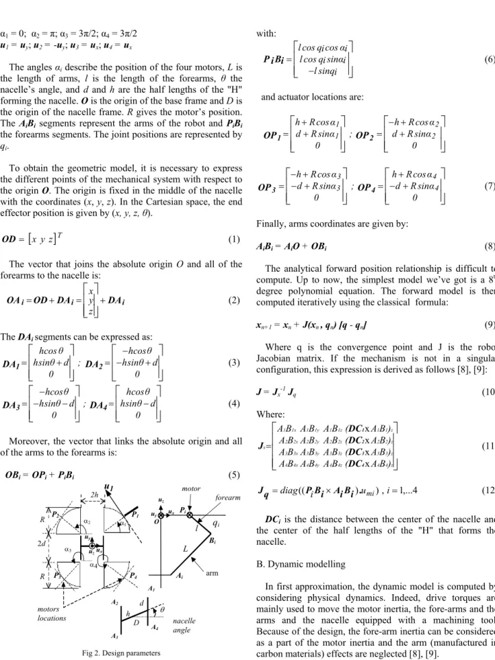
The Jacobian matrix and the forward geometric model are needed to compute the dynamic model (see section 2.2). Therefore we briefly present the way of computing the different relationship necessary to obtain these model and matrix. The design parameters of the robot are described on Fig. 2 where the following parameters have been chosen:
Proceedings of the 2003 IEEE
International Conference on Robotics & Automation Taipei, Taiwan, September 14-19, 2003
α1 = 0; α2 = π; α3 = 3π/2; α4 = 3π/2
u1 = uy; u2 = -uy; u3 = ux; u4 = ux
The angles αi describe the position of the four motors, L is
the length of arms, l is the length of the forearms, θ the nacelle’s angle, and d and h are the half lengths of the "H" forming the nacelle. O is the origin of the base frame and D is the origin of the nacelle frame. R gives the motor’s position. The AiBi segments represent the arms of the robot and PiBi
the forearms segments. The joint positions are represented by
qi.
To obtain the geometric model, it is necessary to express the different points of the mechanical system with respect to the origin O. The origin is fixed in the middle of the nacelle with the coordinates (x, y, z). In the Cartesian space, the end effector position is given by (x, y, z, θ).
[
x y z]
T=
OD (1)
The vector that joins the absolute origin O and all of the forearms to the nacelle is:
OAi=OD+DAi= +DAi (2)
z y xThe DAi segments can be expressed as:
+ −− = + = 0 d sinθ h θ cos h ; 0 d sinθ h θ cos h DA DA1 2 (3)
− = − −− = 0 d sinθ h θ cos h ; 0 d sinθ h θ cos h DA DA3 4 (4)Moreover, the vector that links the absolute origin and all of the arms to the forearms is:
OBi = OPi + PiBi (5)
Fig 2. Design parameters
with: (6)
− = i sinq l i sinα i q cos l i α cos i q cos l i B i Pand actuator locations are:
++ − = + + = 0 sinα R d α cos R h ; 0 sinα R d α cos R h 2 2 1 1 OP OP1 2
+ −+ = + − + − = 0 sinα R d α cos R h ; 0 sinα R d α cos R h 4 4 3 3 OP OP3 4 (7)Finally, arms coordinates are given by:
AiBi = AiO + OBi (8)
The analytical forward position relationship is difficult to compute. Up to now, the simplest model we’ve got is a 8th
degree polynomial equation. The forward model is then computed iteratively using the classical formula:
xn+1 = xn + J(xn , qn) [q - qn] (9)
Where q is the convergence point and J is the robot Jacobian matrix. If the mechanism is not in a singular configuration, this expression is derived as follows [8], [9]:
J = Jx-1 Jq (10) Where:
= z 4 4 4z 4 4y 4 4x 4 z 3 3 3z 3 3y 3 3x 3 z 2 2 2z 2 2y 2 2x 2 z 1 1 1z 1 1y 1 1x 1 x ) B A ( B A B A B A ) B A ( B A B A B A ) B A ( B A B A B A ) B A ( B A B A B A x x x x 4 3 2 1 DC DC DC DC J (11) 4 ,... 1 , ) ) (( ×.
= =diag PiBi AiBi umi i q J (12)DCi is the distance between the center of the nacelle and
the center of the half lengths of the "H" that forms the nacelle.
B. Dynamic modelling
In first approximation, the dynamic model is computed by considering physical dynamics. Indeed, drive torques are mainly used to move the motor inertia, the fore-arms and the arms and the nacelle equipped with a machining tool. Because of the design, the fore-arm inertia can be considered as a part of the motor inertia and the arm (manufactured in carbon materials) effects are neglected [8], [9].
uz 1 u motor 2h u z forearm ux Pi uy P2 P1 O R α2 α1 α3 P4 P3 uy ux A3 A2 A1 L l Bi qi 2d α4 arm Ai R d h θ motors locations D nacelle angle A4
3279
If Γmot is the (4x1) actuator torque vector, the basic
equation of dynamics can be written as :
) sign( G) ( v c mot mot I q JTMx Fq F q
Γ = &&+ &&− + & + & (13) where Imot represents the motor’s inertia matrix including the
forearm’s inertia, M a matrix containing the mass of the nacelle and its inertia, q is the (4x1) joint velocity vector, is (4x1) the joint acceleration vector , is the vector of cartesian accelerations, and G the gravity constant. Thanks to the design, the forearm’s inertia is taken into account in the motor’s inertia. F
& q&&
x&&
v are the viscous friction coefficients and Fc
are the Coulomb friction. With:
= mot4 mot3 mot2 mot1 mot I 0 0 0 0 I 0 0 I 0 0 0 0 0 0 II
(14)
=
bc I nac M nac M nac M 0 0 0 0 0 0 0 0 0 0 0 0 M (15)It is first assumed that the nacelle acceleration and the motor position
are directly measured. The dynamic equation can be rewritten in a relation linear to the dynamic parameters. By introducing
[
Tθ z y x&& && && && && = x
[
q1 q2 q3 q = q]
]
T 4[
T T]
T 41 43J
J
J
=
, it follows:X
q
q
J
J
q
Γ
−
=
43 41&&
&
(
&
)
&&
&&
&&
&&
sign
G
z
y
x
T T motθ
(16)where X is the vector of parameters:
bc nac mot mot mot mot I I I M I I 1 2 3 4 [ = X T c c c c v v v v
F
F
F
F
F
F
F
F
1 2 3 4 1 2 3 4]
(17)If acceleration measurement & is not available, & can be
evaluated by: x& x&
[
Tq q q q y z
x&& && && θ&&
& & && &&=Jq+Jq=
x
]
(18)where depends on x and q, is computed using a central difference algorithm.
J
J&
Then, the second identification dynamic model is given by :
X − = sign( ) G zy x q q q q q θ J J q 43 41 q
Γ && & &
&&&& &&
&& T T
mot (19)
Both models are expressed in a general form: X
D
Y= (20)
where Y is the torque measurement vector, D is called the regressor and X is the vector of unknown parameters.
III. IDENTIFICATION METHOD
The identification technique, classically developed for robot manipulators, is applied for the parallel robot. Usually X is estimated as the least squares (LS) solution of an over-determined linear system obtained by sampling and filtering the dynamic model (20) along a trajectory ( , considering that ρ is a zero mean additive independent noise, with a standard deviation σ
) , , qq q & && ρ such that: Cρρ = E(ρTρ) = σρ2Ir (21)
where E is the expectation operator. Ir is the (rxr) identity
matrix. The over-determined system is written as follows:
Y = W X + ρ (22)
where Y is the (rx1) measurement vector, W is the (rxN) observation matrix, N is the number of parameters to identify. In fact Y is obtained by concatenation of n measurements vectors Yj of the n motor torques with different error standard
deviations. A better solution is to calculate the WLS solution of the global system (22). The rj rows, corresponding to joint
j equation, are weighted by the coefficient of the diagonal
matrix of the error covariance matrix defined as follows: Cρρ = (GT G)-1 G = diag(S) (23)
G is a (rxr) diagonal matrix composed of the elements of S.
[
]
= = 1 n j j ρ σ 1 ρ σ 1 , S S ˆ ˆ K K Sj S (24)Sj is a (lxrj) row matrix. An unbiased estimation
ρ
σˆ j is used
from the regression on each joint j subsystem:
2 j j j j j 2 j p N r Θ Φ Y ρ σ
− − = ˆ ˆ (25) j j j j j Φ Θ r NpY , , , , are the measurement vector, the
of minimum parameters for each joint j subsystem respectively.
The WLS vector solution minimizes the Euclidean norm of the vector of weighted errors ρ:
w Xˆ
[
ρ G Gρ]
X Arg.min T T = w Xˆ (26) wXˆ and the corresponding standard deviations σ are calculated as the LS solution of (22) weighted by G:
wi Xˆ
Yw = WwX + ρw
(27) Yw = GY, Ww = GW, ρw = Gρ
Complete details concerning the WLS identification technique and its practical implementation can be found in [10], [11], [12].
IV. EXPERIMENTAL RESULTS A. Determination of the amplifier gain
For industrial robots, torques are usually estimated using a linear relation between torque and voltage applied to the amplifier: T T m = G V Γ (28)
where VT is the current reference of the amplifier current loop
and GT the gain of the joint drive chain. A good estimation of
GT is important to obtain a good estimation of the physical
parameters.
A force sensor, located on the nacelle, is used to measure directly the force produced at the arm end. Applying different input tensions to the amplifier, the resulting torques are measured and the gain is estimated (Table 1). In [10], other techniques to estimate the GT values are given.
B. Dynamic parameters estimation
In this work, we are focused in the estimation of the following dynamic parameters:
bc nac mot mot mot mot I I I M I I 1 2 3 4 [ = X
]
4 3 2 1 4 3 2 1 v v v c c c c vF
F
F
F
F
F
F
F
(29) TABLE 1 AMPLIFIERS GAINSMotor 1 Motor 2 Motor 3 Motor 4
GT (N.m/V) 2.85 2.65 2.70 2.87
For computing the regressor, joint velocities and accelerations are estimated by a band pass filtering of the position. The band pass filtering is obtained by the product of a low pass filter in both the forward and the reverse direction (Butterworth) and a derivative filter obtained by a central difference algorithm, without phase shift. A parallel filtering is implemented to reject the high frequency ripples of the measured motor torques. Practical aspects of the derivative estimation and data filtering are completely detailed in [13] and [14].
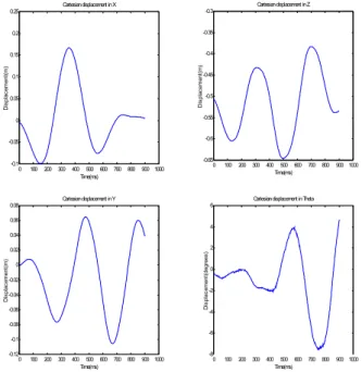
In order to get good identification results, exciting trajectories containing slow motions (in such a case, friction will be preponderant) and high dynamic motions (inertia phenomena become preponderant) are generated. Finally, concatenation of these trajectories is used. Examples of generated trajectories are presented in Fig. 3.
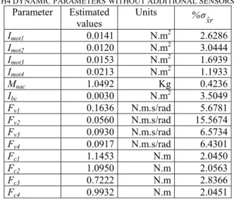
1) Identification without additional sensor: Initially, the Cartesian accelerations are computed thanks (18), where the actuator velocities and accelerations have been computed from the actuators positions. Table 2 shows the obtained parameters of the dynamics model (19). The relative standard deviation ( %σxˆr) is given.
The physical parameters are quite well estimated in comparison to the prior values of nacelle mass and the motor inertia (0.975 Kg and 0.012 N.m2 respectively). However
additional measurements are provided to improve estimation accuracy.
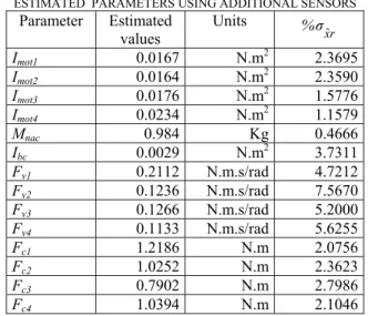
2) Identification using additional sensors: An accelerometer located on the nacelle gives the Cartesian accelerations on the
0 100 200 300 400500 600 700 800 900 1000 -0.65 -0.6 -0.55 -0.5 -0.45 -0.4 -0.35 -0.3 Cartesian displacement in Z D isp la ce m en t( m ) Time(ms) 0 100 200 300 400500 600 700 800 900 1000 -0.12 -0.1 -0.08 -0.06 -0.04 -0.02 0 0.02 0.04 0.06 0.08 Cartesian displacement in Y D isp la ce m en t( m ) Time(ms) 0 100 200 300 400500 600 700 800 900 1000 -8 -6 -4 -2 0 2 4
6 Cartesian displacement in Theta
Time(ms) D is pl ac em ent (degr ees ) 0 100 200 300 400 500 600 700 800 900 1000 -0.1 -0.05 0 0.05 0.1 0.15 0.2 0.25 Cartesian displacement in X Time(ms) D isp la ce m en t( m )
Fig. 3 Typical trajectories in the Cartesian space
TABLE 2
H4 DYNAMIC PARAMETERS WITHOUT ADDITIONAL SENSORS Parameter Estimated values Units %σxˆr Imot1 0.0141 N.m2 2.6286 Imot2 0.0120 N.m2 3.0444 Imot3 0.0153 N.m2 1.6939 Imot4 0.0213 N.m2 1.1933 Mnac 1.0492 Kg 0.4236 Ibc 0.0030 N.m2 3.5049 Fv1 0.1636 N.m.s/rad 5.6781 Fv2 0.0560 N.m.s/rad 15.5674 Fv3 0.0930 N.m.s/rad 6.5734 Fv4 0.0917 N.m.s/rad 6.4301 Fc1 1.1453 N.m 2.0450 Fc2 1.0950 N.m 2.0563 Fc3 0.7222 N.m 2.8366 Fc4 0.9932 N.m 2.0451
three axes (x, y and z) and a rotation sensor gives the central bar rotation. We use them to perform the identification straight with the model of (19). Fig. 4 shows the comparison of measured data obtained from the accelerometer and rotation sensor and those provided by (16). Rotation acceleration is numerically computed by a finite central difference.
Table 3 shows the fourteen estimated parameters of the dynamic model (16). In case of the rigid multi body model identification, additional sensors located on the end effector mainly improve the estimation of the viscous friction coefficients and their relative standard deviations.
C. Experimental validation
The validation of the identification results consists in comparing the measured torques with those obtained by computing the inverse dynamic model with the estimated parameters. Fig. 5 exhibits cross validations with new trajectories that have not been used previously for the identification. Simulation and measurements are very close. The dynamic parameters are quite well estimated.
These experiments show good results of the dynamic identification. The use of the accelerometer and rotation sensor are not very necessary for the rigid model.
V. CONCLUSION
In this paper experimental results related to the identification of physical dynamic parameters of a fully parallel robot are presented. Estimated values depending on the available measurements at the end effector are exhibited. The cross validation shows good identification results.
0 100 200 300 400 500 600 700 800 900 1000 -10 -8 -6 -4 -2 0 2 4 6
8 A x e X: - M eas ured ac c elerations -- Calc ulated ac c elerations
Tim e(m s ) A cce le ra tio ns( m /s2 ) 0 100 200 300 400 500 600 700 800 900 1000 -40 -30 -20 -10 0 10 20 30
40 A x e Y : - M eas ured ac c elerations -- Calculated ac celerations
A cce le ra tio ns( m /s2 ) Tim e(m s) 0 100 200 300 400 500 600 700 800 900 1000 -150 -100 -50 0 50 100
150 A x e Theta: - M eas ured ac c elerations -- Calc ulated ac c elerations
A cce le ra tio ns( m /s2 ) Tim e(m s ) 0 100 200 300 400 500 600 700 800 900 1000 -50 -40 -30 -20 -10 0 10 20 30 40 50
A x e Z: - M eas ured ac c elerations -- Calc ulated ac c elerations
Tim e(m s ) A cce le ra tio ns( m /s2 )
Fig. 4 Calculated and measured accelerations
However this structure working with high speed and acceleration presents important flexibility and slight differences during validation may be due to flexibility. Therefore, we are currently working on the introduction of lumped elasticities in the dynamic model. In the future, we will compare the results with other estimation methods and this complete dynamic model will be used in model based control scheme with moving horizon for machining tasks.
TABLE 3
ESTIMATED PARAMETERS USING ADDITIONAL SENSORS Parameter Estimated values Units %σxˆr Imot1 0.0167 N.m2 2.3695 Imot2 0.0164 N.m2 2.3590 Imot3 0.0176 N.m2 1.5776 Imot4 0.0234 N.m2 1.1579 Mnac 0.984 Kg 0.4666 Ibc 0.0029 N.m2 3.7311 Fv1 0.2112 N.m.s/rad 4.7212 Fv2 0.1236 N.m.s/rad 7.5670 Fv3 0.1266 N.m.s/rad 5.2000 Fv4 0.1133 N.m.s/rad 5.6255 Fc1 1.2186 N.m 2.0756 Fc2 1.0252 N.m 2.3623 Fc3 0.7902 N.m 2.7986 Fc4 1.0394 N.m 2.1046 VI. REFERENCES
[1] V.E. Gough, “Contribution to discussion of papers on research in automotive stability, control and tyre performance”, Proc. Auto Div., Inst. Mechanical
Engineers, 1956-1957.
[2] D. Stewart, “A plataform with 6 degrees of freedom”,
Proc. of the Ins. of Mech. Engineers, 180 (Part 1, 15), pp.
371-386, 1965.
[3] R. Clavel, “Une nouvelle structure de manipulateur parallèle pour la robotique légère”, APII, 23 (6), pp. 501-519, 1989.
[4] J.-P. Merlet, Les robots parallèles, 2nd Edition, Hermes,
1997.
[5] H. K. Tönshoff, “A systematic comparison of parallel kinematics”, Keynote in proceedings of the first forum on
parallel kinematic machines, Milan, Italy, August 31 –
September 1, 1998.
[6] F. Pierrot, T. Shibukawa, “From Hexa to HexaM”, Proc.
IPK’98: Internationales Parallelkinematik-Kolloquium,
Zürich, June 4, pp. 75-84, 1998.
[7] F. Pierrot, P. Dauchez and A. Fournier, “Fast parallel robots”, Journal of robotics systems, 8 (6), pp. 829-840, 1991.
[8] O. Company, F. Pierrot, “A new 3T-1R parallel robot”,
ICAR’99, Tokyo, Japan, October 25-27, pp. 557-562,
1999.
[9] F. Pierrot, F. Marquet, O. Company, T. Gil, "H4 Parallel Robot,: Modeling, Design and Preliminary Experiments",
Proc. of the 2001 IEEE International Conference one Robotics & Automation, Seoul, Korea, May 21-26, 2001.
[10] P. Restrepo, “Contribution à la modélisation, identification et commande des robots à structures fermées: application au robot ACMA SR400”, Ph.D
Thesis, Ecole Centrale de Nantes, France, 1996.
[11] Ph. Poignet, M. Gautier, "Extended kalman filtering and weighted least squares dynamic identification of robots”,
Control Engineering Practice, 2001, vol. 9/12, pp. 1361-
0 1 0 0 2 0 0 3 0 0 4 0 0 5 0 0 6 0 0 7 0 0 8 0 0 9 0 0 1 0 0 0 -8 -6 -4 -2 0 2 4 6 M o t o r 1 : - C a lc u la t e d t o rq u e -- M e a s u re d t o rq u e T im e (m s ) To rq ue (N .m ) 0 1 0 0 2 0 0 3 0 0 4 0 0 5 0 0 6 0 0 7 0 0 8 0 0 9 0 0 1 0 0 0 -8 -6 -4 -2 0 2 4 M o t o r 2 : - C a lc u la t e d t o rq u e -- M e a s u re d t o rq u e T orq ue (N .m ) T im e (m s ) 0 1 0 0 2 0 0 3 0 0 4 0 0 5 0 0 6 0 0 7 0 0 8 0 0 9 0 0 1 0 0 0 - 8 - 6 - 4 - 2 0 2 4 6 8 T i m e (m s ) T orq ue (N .m ) M o t o r 3 : - C a lc u la t e d t o r q u e - - M e a s u re d t o r q u e 0 1 0 0 2 0 0 3 0 0 4 0 0 5 0 0 6 0 0 7 0 0 8 0 0 9 0 0 1 0 0 0 - 8 - 6 - 4 - 2 0 2 4 6 8 M o t o r 4 : - C a lc u la t e d t o r q u e -- M e a s u r e d t o r q u e T orq ue (N .m ) T im e ( m s )
Fig. 5 Calculated and measured torques 1372.
[12] C. Canudas de Wit, B. Siciliano, G. Bastin, Theory of
robot control, Springer, 1996.
[13] W. Khalil, E. Dombre, Modeling, Identification and
Control of Robots, Hermes Penton Science, London,
2002.
[14] M.T. Pham, M. Gautier, Ph. Poignet, “Dynamic identification of high speed machine tools”, Proc. of the II
International Seminar on Improving Machine Tools Performance, La Baule, France, 2000.