Assessment of Spatial Variability of the corrosion of steel infrastructures from Ultrasonic measurements: application to coastal infrastructures

HAL Id: hal-01007914

https://hal.archives-ouvertes.fr/hal-01007914

Submitted on 28 Aug 2018

HAL is a multi-disciplinary open access archive for the deposit and dissemination of sci-entific research documents, whether they are pub-lished or not. The documents may come from teaching and research institutions in France or abroad, or from public or private research centers.

L’archive ouverte pluridisciplinaire HAL, est destinée au dépôt et à la diffusion de documents scientifiques de niveau recherche, publiés ou non, émanant des établissements d’enseignement et de recherche français ou étrangers, des laboratoires publics ou privés.

Assessment of Spatial Variability of the corrosion of

steel infrastructures from Ultrasonic measurements:

application to coastal infrastructures

Franck Schoefs, Trung-Viet Tran

To cite this version:

Franck Schoefs, Trung-Viet Tran. Assessment of Spatial Variability of the corrosion of steel infrastruc-tures from Ultrasonic measurements: application to coastal infrastrucinfrastruc-tures. International Conference on Structural Safety & Reliability (ICOSSAR’11), 2013, New York, United States. pp. 2697-2704. �hal-01007914�

1 INTRODUCTION

Steel structures in sea or estuary area are subjected to corrosion process. The phenomenon is very com-plex due to the nature of the environment and mate-rial, and the type of the structure. This phenomenon needs to be characterized and modeled for structural analysis which accounts for the loss of thickness. Moreover, due to the randomness of the corrosion process, probabilistic models are needed for struc-tural reliability (Boéro 2012). Ultrasonic residual measurements allow determining profiles of loss of thickness, identifying the areas which are the most affected by corrosion and stating the assumptions for modeling the random corrosion process. Several in-spection campaigns have been performed during the three last decades in some French harbours. Thus a great number of ultrasonic residual measurements are now available for structures in various environ-ments. The protocol is recommended by the CET-MEF (French Center for Maritime and Fluvial Tech-nical Studies :Engineering centre of the French Ministry of Public Works): at a given level, this pro-tocol suggest to perform three geometrical meas-urements at a given location to assess the loss of thickness as the average of these three readings. Generally, the amount of data is more than 1000 per structure and allows performing a statistical analysis of the spatial distribution of the loss of thickness ac-cording to the different areas (mainly tidal and im-mersion areas). Moreover environmental parameters (temperature, PH, oxygen, salinity, conductivity, nu-trients) have been measured since a decade and are available.

This study began within the MEDACHS frame-work (Marine Environment Damage to Atlantic Coast Historical and transport works or Structures-Interreg IIIB Project funded by EC 2005-2007) and is performed now in the GEROM framework (Risk management of French harbor structures: stakes, current practices and needs – Experience feedback of owners). The steel structures are sheet-piles, on-pile and on-sheet-on-pile wharves. This paper focuses on sheet-piles seawalls and coffer-dams. More than 35 000 data are available: they correspond to meas-urements in 4 harbours and concern more than 20 quays (Boero et al. 2009a, 2009b). This paper focus-es on the spatial dependence of the corrosion procfocus-ess and we present only results of three of them where the distance between data is small (0.20 m horizon-tally and 0.10 m vertically).

In the first part, the paper presents the data avail-able (Euromarcorr data base) to study the spatio(-temporal) fields of corrosion for steel sheet-piles.

The next part presents the geo-statistical model-ing of the spatial variability of the steel sheet piles corrosion; and more particularly the study of the sta-tionary of the process of corrosion according to the length.

We suggest a three scale modeling of spatial vari-ability of corrosion base on a study case.

Finally, from identification of parameters of a sta-tionary stochastic field, we suggest an optimization of the inspection.

Assessment of Spatial Variability of the corrosion of steel infrastructures

from Ultrasonic measurements: application to coastal infrastructures

F. Schoefs & T.V. Tran

LUNAM Université, Université de Nantes, Institute for Research in Civil and Mechanical Engineering, CNRS UMR 6183, Nantes, France

ABSTRACT: Corrosion is one of the major causes of degradation for harbor structures. The time variant modeling is still a challenge due to the complexity of phenomena and the number of physical and electro-chemical equations that govern the corrosion process and that are competing with each other. That emphasiz-es the role of condition assemphasiz-essment from on-site measurements as the unique input for maintenance decision. The cost of inspection of marine structures being prohibitive, owners required decision aid-tool for optimizing this step of the maintenance process. After a brief description of the existing data-base in France, this paper is devoted to the optimization of ultra-sonic measurements by considering the spatial variability measured from real data for each zone of corrosion.

2 EUROMARCORR DATA BASE

2.1 Medium and long-term orrosion data -base Corrosion measurements are collected on two types of marine structures: on-pile wharves and on-sheet pile wharves. Structures are located on the French coasts, i.e. Atlantic, Channel and Mediterranean coasts. In this paper, only corrosion measurements associated to steel sheet piles are presented.

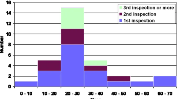
Almost all the studied structures were built be-tween 1955 and 1985. Only three structures are older than 1955 and none is more recent than 1985. The owners began NDT measurements of residual thick-nesses from 1990. Consequently most of the struc-tures are 10 to 40 years old at the inspection time: medium an long-term corrosion can be analysed. Figure 2 presents the distribution of the age of the structures at the first, second, third and more inspec-tion times.

Figure 2. Age distribution of the studied structures at inspec-tion time.

Four harbours are considered and called BO, HA, PL, SE. The distribution of the structures within the studied harbours and according to the type of water variation (dock at constant seawater level, wet dock and tidal dock) is presented on figure 3.

Figure 3. Harbours and docks distribution.

Over a total amount of 23 structures, 11 are locat-ed in docks at constant seawater level, 9 in tidal docks and 3 in wet docks. In this last case the water

level changes with the same period as the tide but with lower amplitude.

The variation of the seawater level in the various docks is detailed on figure 4.

The tide level corresponds to the range between the HAT (Highest Astronomical Tide) and the (LAT (Lowest Astronomical Tide).

Figure 4. Harbours and docks distribution.

The variation of the height of water is important in tidal docks of BO and HA harbours. The variation is of course weaker in harbours located along the Med-iterranean coast (i.e. PL and SE harbours).

Most of the measurements are made in the im-mersed zone, including the zone of low seawater level and the mud zone. Only the HA harbour began some measurements in the tidal/spray and in the at-mospheric zones. The amount of data according to the studied harbours and for the various exposure zones is detailed on the figure 5.

zones is detailed on the figure 5.

Figure 5. Distribution of data (loss of thickness) in the various exposure zones.

The structure of the BO harbour was alone the sub-ject of large campaign of measurements: it repre-sents 99 % of all the available measurements.

2.2 Corrosion measurements

Corrosion of steel structures is classically assessed by ultrasonic non destructive testing. In France, a protocol is given by the CETMEF and classically used by several companies to perform inspections of coastal steel structures. The CETMEF is part of the

French ministry of building. It is devoted to the dif-fusion of knowledge, to provide technical and search studies as well as engineering and expert's re-ports. This protocol consists in performing residual thickness measurements for several heights of the structure using ultrasonic testing. The corrosion products are removed by grinding. By using this technique and considering the harsh conditions for marine inspections, the error on the measurements at a given point on the structure cannot be neglected. Error comes both from the physical measurement (around 0.1 mm) and from the protocol (grinding, link diver-operator, etc.). Thus three measurements are performed on a given location: the three meas-urements are distributed on a circle, with diameter of about 5 cm, every 120° as shown on figure 1. The average of these three readings is considered as the “true” loss of thickness. For on-pile wharves, in view to analyze the corrosion around the pile, meas-urements are performed at several cardinal positions of the pile's section (see figure 1). For on-sheet-pile-wall wharves, they are performed along the length of the wharf around every 10 meters, which is classi-cally the mean distance between two piles for on-pile wharves. Starting from these residual thickness values, and knowing the initial thickness of piles or sheet-piles, we deduce the thickness loss mainly due to corrosion. This protocol involves recommenda-tions only and in some cases, this protocol is not fol-lowed because of the experience of owners or the re-sults of the risk based inspection analysis. That is the case for structures considered in the lat part of the structures where the distance between measurements is closer.

Figure 1. CETMEF protocol: cardinal points for pile (left) and location for sheet pile (right).

2.3 Selected structures for spatial variability

The study of the spatial variability of corrosion is performed from the data of three structures extracted from the database. This selection is based on the fact that the distance between horizontal or vertical measurements are much weaker than everywhere else. Consequently, the quantity of information is consequent to perform a spatial analysis of the cor-rosion process.

In the three cases, it is important to remind that these specific campaigns were devoted to the discovery of perforations on steel sheet piles. In the case of the structure HA7d, the control was also started after the observation of accidental acids discharges.The main technical characteristics of these structures are de-tailed in tables 1. Table 2 gives more details con-cerning the type of sheet piles and the auscultation strategy.

Table 1. Characteristics of the selected structures. ______________________________________________ Structure BO1 HA7d HA8b ______________________________________________ Function General General General

cargo cargo cargo Type Cofferdam Seawall Seawall Sheet piles Flat U-sections U- sections Width (m) 0.5 0.5 0.5 Length (m) 758 (1230*) 345 187 Age (Years) 25 28 26 Sea Channel Channel Channel Dock type Tidal Constant Constant

seawater seawater level level Seawater

variation level 9.1 0.6 0.6 _____________________________________________ *wrap around distance for Cofferdam

Table 2. Corrosion measurements strategies of the selected structures.

______________________________________________ Structure BO1 HA7d* HA8b ______________________________________________ Location of measurements

on steel sheet piles - In & out Out-pans pans

Length of the measured

part of the structure (m) 991.3 35.0 123.0 Height of the measured

part of the structure (m) 3.0 9.6 6.1 Number of measurements

following length 5988 71 36 Mean horizontal spacing

between measurements (m) 0.15 0.5 3.5 to 0.2

Number of measurements

following depth 7 13 48 Mean vertical spacing

between measurements (m) 0.5 0.8 0.1 Number of loss thickness

measurements 32238 685 504 Measurements location in

several exposure zones** T, L, I L, I L, I ______________________________________________ Tidal zone ZT

______________________________________________ Number of measurements

following depth 2 - - Number of loss thickness

Measurements 11073 - - Percentage of

the total amount of

measurements 34 - - ______________________________________________ Low seawater zone ZL

______________________________________________ Number of measurements

following depth 1 4 2 Number of loss thickness

Measurements 5350 220 24 Percentage of

the total amount of measurements 17 32 4 ______________________________________________ Immersion zone ZI ______________________________________________ Number of measurements following depth 4 9 46 Number of loss thickness

Measurements 15815 465 480 Percentage of

the total amount of

measurements 49 68 96 _____________________________________________ *Measurements alternatively on in and out -pans of U-shape sheet piling.

** ZT = Tidal zone; ZL = Low seawater zone; ZI = Immersion zone.

2.4 Environment of selected structures

The physico-chemical parameters of seawater near the studied structures are described on table 3. Most of them were measured between 1997 and 2007.

Table 3. Mean values and ranges of physico-chemical parame-ters of seawater near the studied structures.

______________________________________________ Structure BO1 HA7d & HA8b _______________ ______________ Parameter Mean Min Max Mean Min Max ______________________________________________ Temperature (°C) 13.3 7.2 19.5 13.7 8.1 20.7 pH 8.0 7.8 8.1 8.1 7.7 8.5 Conductivity (mS/cm) 49.0 46.8 50.5 37.2 33.7 41.4 Salinity (g/l) 32.9 31.5 33.7 25.4 23.9 27.7 O2 (mg/l) 8.7 6.4 11.2 8.7 6.9 11.0 SM* (mg/l) 9.9 4.7 17.7 8.3 3.3 15.0 NH4 (mg/l) 0.5 0.2 0.9 0.3 0.1 0.6 NO2 (mg/l) 0.2 0.1 0.3 NO3 (mg/l) 6.4 2.6 8.8 PO4 (mg/l) 0.4 0.1 0.6 _____________________________________________ *SM = Suspended materials.

The physico-chemical parameters of seawater for the structures HA7d and HA8b are identical because they are located in the same dock.

3 MODELING SPATIAL VARIABILITY FROM MEASUREMENTS

3.1 Data pre-processing

The loss of thickness on each location is computed by averaging the three readings corresponding to three positions occupied by the ultrasonic transducer inside the required location (see figure 1).

Sometimes, for technical reasons, a single basic measurement is realized in a location. In that case, the loss of thickness which characterizes this loca-tion was removed from the database because the er-ror can be significant.

Moreover, perforations were observed on steel sheet piles. The loss of thickness cannot be meas-ured in that case and the corresponding data were al-so removed for the statistical analysis.

To analyze the influence of the physico-chemical parameters on the corrosion mechanism in marine environment, the following hypotheses will be veri-fied in the future:

! The temporal series of the physico-chemical pa-rameters of the seawater follow a stationarity pro-cess (no trend or jump). The hypothesis of the stationarity or non-stationarity can be verified by an appropriate test;

! The absence or low influence of the depth on the physico-chemical parameters. We don’t have any measure of these parameters along the wharf length;

! The homogeneous distribution of the measures of the seawater quality during the various seasons is necessary to make sure that the statistical charac-teristics of the parameters are not biased. It can easily be verified or corrected.

3.2 Analysis of the spatial variability of the

corrosion process

The “loss of thickness” due to the corrosion is con-sidered here as a stochastic field indexed by the space at the inspection time. Due to the corrosion process, we consider here that the principal direc-tions are known: x, along the wharf length and z, along the wharf depth.

From the available distances between measure-ments, the objective is here to analyse if the corro-sion is or not a second-order stationarity process in R ! i.e. according to the two coordinates x and z (see figure 6).

figure 6).

Figure 6. Study of the stationarity of the corrosion process ac-cording to the direction x (a) and the direction z (b).

For that purpose, three conditions are to be verified: ! (i) The arithmetic mean of the marginal variables

must be constant according to the studied direc-tion;

! (ii) The variance of the marginal variables must be constant according to the studied direction too. If not, the random process is not stationary. If yes and if the first condition is not verified, the field can be centered and the further analysis is made on the remainder;

! (iii) The covariance depends only on the distance between points according to the studied direction_!"

3.3 Spatial variation according to z

This question is under investigation since a dec-ade now in France first by Memet (2000) and more recently by Boéro (2010). It was identified already in the 50’s by Larrabee and LaQue in USA (LaQue 1948, Larrabee 1958). This is described more in de-tail in Boéro et al. (2009c). For the moment, the complexity of phenomena involved has been identi-fies in each of the 7 zones i.e. from top to bottom: Aerial, High level of tide, Tide, Low level of tide, Immersion, Mud, and Soil. Due to the number of random influencing factors varying with time no complete modeling is actually available: for in-stance, in the area “low level of tide” the abrasion can be due to the sand mining during a specific length of time. Phenomenological models suggested by Melchers (1999) and Melchers & Jeffrey (2008) or statistical models suggested by Boéro (2012) are probably the best ones for long term modeling of the corrosion of harbor structures. Figure 7 provides the usual form of the corrosion (Boéro et al. 2012) with 6 area from the 7 presented upon: only “High level of tide” is absent (around depth -2m). Note that due to the lack of knowledge of the modeling in each ar-ea a piecewise stationary process can be suggested, except in the immersion area (from depth 6 to -11.5m) for which we now that the corrosion is de-creasing with depth due to the diminished dissolved di-oxygen availability. As the corrosion peak loca-tions are known and the depth limited to several me-ters, the inspection with depth is not so challenging than the inspection along the length for structures of several hundred meters length. That is why we focus on this aspect mainly in the following.

!24 !22 !20 !18 !16 !14 !12 !10 !8 !6 !4 !2 0 0 1 2 3 4 5 6 7 8 9 10 D ep th 1(m ) Loss1of1thickness1(mm) Mean1! t10 Mean1! t25 Mean1! t50 Quant.195%1! t10 Quant.195%1! t25 Quant.195%1! t50

Figure 7. Mean value and 95% quantiles of steel thickness loss in each zone at time 10, 25 and 50 years.

3.4 The 3 scales spatial variation according to x Three scales of spatial variation have been identified (Boéro et al. 2009c): the scale of the shape of the sheet pile (U type), the regular part of the wall and special areas as the joints area between cofferdams or ends of the wharf. We focus in this paper on the regular part.

3.5 Assessment of stochastic field properties from

measurements

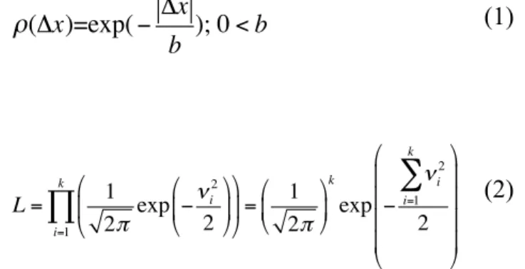
Properties (i) and (ii) have already been proved in Boéro et al. 2009c and we focus in this paper on the assessment of the auto-correlation ρTT. In view to optimize the inspection we need to model the field. If the stationarity is confirmed (first studies by Boéro et al. 2009c) several methods are available to identify the parameters of a correlation function. Two major procedures have been reported in the lit-erature for the estimation of δ for a spatially variable property from a digitized record of data. In the first procedure, reported by Li (2004), the Maximum Likelihood Estimate method (MLE) is used in which different values for the model parameter of the pro-posed ACF model is assumed and the value that maximizes the corresponding MLE is taken as the model parameter. In the second procedure, proposed by Vanmarcke (1983) and applied in Schoefs et al. (2011b), a proposed ACF model can be adjusted to provide the best fit to the actual sample correlation coefficients ρ(Δx) thereby providing estimates of the corresponding model parameter (i.e. b in (1)). This last one can lead to a biased estimation when data are lacking. In this paper, we select an exponential ACF (Eq. (1)) and we use the MLE for the estima-tion of b (2). ρ(Δx)=exp( − Δx b ); 0 < b (1) L = 1 2π exp − νi 2 2 " # $ % & ' " # $ % & ' i=1 k

∏

∑

where νi is the ith component of the vector of

in-dependent standard values obtained from equation: ν = C−1 T − µˆ _Tˆ σ_Tˆ " # $$ % & '' (3)

where _Tˆ _{is the vector of realizations after}

inspec-tion of the random variable Z and C a lower triangu-lar matrix such that CCT= ρ and ρ the autocorrela-tion matrix. Beside, maximize L is equivalent to minimize L1:

∑

4 PRACTICAL STUDY CASE FOR STOCHASTIC FIELD MODELLING 4.1 Identification of a regular part

We select here the cofferdam BO1 structure due to the low spacing between measurements (15 to 20 cm), 25 years old for which long-term corrosion mechanisms is installed, the its length of 1000 me-ters and the flat shape of the sheet-piles: that avoid the local effects due to U-shape sheet piles. A sketch map is presented on Figure 9 where we highlight in the red box an end-effect. Figure 10 pots the corro-sion measures along the whole wharf in the Tidal zone where we observe this end-effect in the red box.

Figure 8. Sketch map of cofferdam BO1.

-1.0 0.0 1.0 2.0 3.0 4.0 5.0 6.0 7.0 8.0 9.0 10.0 0 50 100 150 200 250 300 350 400 450 500 550 600 650 700 750 800 850 900 950 1000 1050 1100 1150 1200 1250 Abscisse x (m) P ert e d'épa is se ur ( m m ) G01 à G50 G101 à G106 Loss of thickness [mm] Abscissa m [m]

Figure 9. Measurements of the loss of thickness along wharf BO1 and end effect (red box).

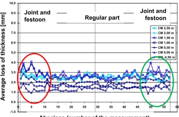
Let us focus on the rest of the structure. It is 22 meters high and is built with 42 gabions of steel sheet-piles and 42 joints between them, called fes-toons (Fig. 10). When analyzing the corrosion in the tidal and immersion zones on a gabion, we observe end-effects too. Figure 11 gathers the average corro-sion trajectories T(x, 25, $i) at 7 positions i in depth for a gabion. The position of the Low seawater zone (ZL) is +1,50 m and the Immersion zone (ZI) is be-low +1 m. It appears (in green and red circles of Figure 10 and 11) that ends-effects due to joint and presence of festoons are particularly pronounced in ZL, which is the zone of higher level of corrosion. Due to the complexity of corrosion phenomena in this area (current, intensive abrasion,…) we dismiss

its analysis in this paper and we focus on what we can now name regular part presented on Figure 10. can now name regular part presented on Figure 10.

Gabion Feston Eau de mer Jonction Parties centrales Parties intermédiaires Gabion Feston Eau de mer Jonction Parties centrales Parties intermédiaires Sea water Regular part festoon Joint

Figure 10. Current part of the cofferdam with gabions, festoons and joints. -1.0 0.0 1.0 2.0 3.0 4.0 5.0 6.0 7.0 8.0 9.0 10.0 0 5 10 15 20 25 30 35 40 45 50 55 60 Abscisse (n° de mesure) Mo ye nne de la per te d'épa is se ur ( m m ) CM 2,50 m CM 2,00 m CM 1,50 m CM 1,00 m CM 0,50 m CM 0,00 m CM -0,50 m

Jonction Partie centrale Jonction

A

verage loss of thickness [mm]

Regular part Joint and

festoon

Joint and festoon

Abscissa (number of the measurement)

Figure 11. Average corrosion along gabions at 7 positions along z-axis.

Note that the mean and the standard deviation can be assumed as constant from the number of meas-urement 10 to 45: that represents 2/3 of the wharf and a length of about 7 meters for the regular part. 4.2 Identification of the stochastic field T

We focus on the auto-correlation in the following. It is plotted on Figure 12 for each of the 7 trajectories presented upon. The shape presents a decreasing with x and can be fitted by a function of x leading to the conclusion that the third property (iii) in section 3.2 is verified.

Figure 12. Experimental auto-correlation at 7 positions along z-axis.

Table 1. Gives the values of b obtained from the fitting of the auto-correlation plots according to sec-tion 3.5. It shows values of similar order of magni-tude from 0.3 to 0.6 with an average value of 0.4.

!"#$% "% "#$% "#&% "#'% "#(% )% *"#""% *)#""% *$#""% *+#""% *&#""% **#""% *'#""% !"#$%&$''()*+$,-. !/ - 012#*,34-.35/-,-./0123-4%$5*% ,-./0123-4%$% ,-./0123-4%)5*% ,-./0123-4%)% ,-./0123-4%"5*% ,-./0123-4%"5"% ,-./0123-4%!"5*%

Table 1. Estimated value of b with depth.

Traj. -0.5 0.0 +0.5 +1.0 +1.5 +2.0 +2.5

b[m] 0.5 0.3 0.4 0.6 0.4 0.4 0.3

5 OPTIMIZATION OF INSPECTION OF A CORROSION STOCHASTIC FIELD 5.1 Method of optimization

After the previous identification part, the objec-tive of this part is to reach the best inspection strate-gy in the regular part for a given goal. The stochastic field being second order stationary we consider a Karhunen–Loève decomposition to generate trajec-tories and simulate inspections on these trajectrajec-tories. We select in this paper a confidence interval of both the mean µ and the standard deviation % expressed as a percentage & of µ and % respectively. We carry out Monte-Carlo simulations to estimate the bounds of the confidence interval for a target probability for the inspection respectively Pti,µ and Pti,%. In a

reliabil-ity study, Pti will be provided by the requirements on the accuracy of the probability of failure assessment. Thus we aim to find the minimum number of inspec-tion along a trajectory and the number of trajectories that allow us to reach the objectives:

P_Tˆ µ = P(!_Tˆ ! (1"#$ "µ)!T;(1+"µ)!T%& (4) P_Tˆ ! = P(!_Tˆ ! (1"

[

]

In the application, target probabilities

Pti,µ=Pti,%=0.85, &µ=0.1 and &%=0.2. These objectives

can be reached only if enough measurements are performed (statistical limitation) and if independant measurements are obtains (correlation limitation). The first one is well known and we focus here on the second one. By knowing the correlation function fit-ted on experimental data in the previous section, the objective will be to get fairly correlated measure-ments in view to obtain a sample: that allows to compute (4) and (5). In view to sample independent events for T, we need to inspect the trajectories with a “sufficiently high distance Lc” to get fairly corre-lated events (Schoefs et al. Unpubl.): it is called IDT for Inspection Distance Threshold. Thus Lc should satisfy: Lc # ]IDT, L[ where L is the potential length of the trajectory, i.e. the maximum inspecta-ble length .

The condition L> Lb is essential to characterize the spatial variability. According to the length of the regular part and results on Table 1, that is the case for the present application. The IDT is defined by assuming that after a given distance, the events measured from an inspection can be assumed as

sta-tistically independent. A Spatial Correlation Thresh-old SCT of the spatial correlation gives this weak correlation. We consider in the following SCT=0.3 that is shown to be optimal by Schoefs et al. (Un-publ.) and seems to be consistent with Figure 12. According to (1), we have the relationship (6) and we obtain IDT=1.2 m and we take Lc=IDT in the fol-lowing.

IDT = b. ln(SCT ) (6)

5.2 Results and analysis

The objective is now to get the optimal quantity of inpections that allows us to reach the objectives of 5.1. We will have to optimize the total number of discrete inspections N=Np*Ns*Nt where Np is the number of repetitive tests for reducing the error of inspection, Ns is the number of inspected sections and Nt the number of trajectories. Here the error of inspection is neglected and Np is not consider. In view to satisfy (4) and (5), the optimal number Nopt is solution of equation (7).

Nopt= argmin

N

max(N!_µ; N !"

(

)

Figure 13 gives the couple of minimum required values for Ns and Nt for the mean value (5) on two positions and the second in the immersion area (-0.5 m) and the second in the tide zone (+2.5 m). Corre-lations function being similar (Table 1), the curves are very close.

Figure 13. Number of required Ns and Nt to ensure Pti,µ =

Pti," = 0.95 (Lc =1.2 m)..

Figures 14 and 15 present the number of total in-spections required as a function of available trajecto-ries (several position along z-axis with a distance of $z if available: $z >Lc) respectively for the

condi-tion on µ (Eq. (4), Fig. 14) and % (Eq. (5), Fig. 15). For z=-0.5, we obtain a total number of 48 with 6 trajectories imposed by the condition on µ and veri-fied by the condition on %. For z=+2.5, we obtain a total number of 44 with 4 trajectories imposed by the condition on µ and verified by the condition on %. For this structure, the effect of the corrosion mecha-nism along z is of minor influence (10 %). Future developments should integrate specific requirements for Pti governed by a reliability analysis that

inte-0 10 20 30 40 50 60 70 80 0 2 4 6 8 10 12 14 Ns N_t !µ=10% Position -0,5 Position 2,5

grates the influence of the position of corrosion (see Boéro et al. 2012).

Figure 14. Required total number of inspection as function of

Nt to ensure Pti,µ = 0.95 (Lc =1.2 m)..

Figure 15. Required total number of inspection as function of

Nt to ensure Pti," = 0.95 (Lc =1.2 m).. 6 CONCLUSION

This paper investigates the scale of corrosion for sheet piles on harbour structures and the requirement for an optimal inspection strategy that accounts for spatial variability.

Two directions of spatial variability are high-lighted: the position in depth with several zones from sol to spray and the position along the length of the wharf. We focus in this paper on this last one were 3 scales of variability are identified: the scale of the sheet-pile (except for flat-shape), scale of the structure (identification of a regular part) and scale of the wharf with end-effects. By focusing on the regular part, it is shown that the stochastic field is second order. This property allows us to generate easily trajectories of this field and simulate inspec-tions. A probabilistic-oriented criteria of the quality of inspection is suggested on the form of a confi-dence interval for both the mean and the standard deviation. Virtual inspection are then carried out and their minimum number required to reach this goal is suggested.

7 REFERENCES

Boéro, J., Schoefs, F., Capra, B., & Rouxel, N. 2009a. Tech-nical management of French harbor structures. Part 1: De-scription of built assets. PARALIA, 2: 6.1–6.11.

Boéro, J., Schoefs, F., Capra, B., & Rouxel, N. 2009b. Tech-nical management of French harbor structures. Part 2: Cur-rent practices, needs – Experience feedback of owners. PARALIA,2: 6.13–6.24.

Boéro, J., Schoefs, F., Melchers, R., & Capra, B. 2009c. Statis-tical analysis of corrosion process along French coast.

ICOSSAR’09. Paper no. 528. Mini-symposia MS15. System

identification.

Boéro, J. 2010. Port infrastructure reliability: innovative ap-proach of analysis and probabilistic modeling of inspection data – Application to the corrosion of metallic structures (in French). Phd thesis. 26 October 2010, University of Nantes. France, p. 450.

Boéro J., Schoefs F., Yáñez-Godoy H., Capra B. 2012. Time-function reliability of harbour infrastructures from stochas-tic modelling of corrosion, European Journal of

Environ-mental and Civil Engineering, 16:10/Nov.2012, 1187-1201.

LaQue, F.L. 1948. Behaviour of metals and alloys in sea water, in: H.H. Uhlig (Ed.). The Corrosion Handbook, John Wiley & Sons, New York, p. 391.

Larrabee, C.P. 1958. Corrosion-Resistant Experimental Steel for Marine Applications, Corrosion, 14, No. 11, 501. Li, Y. 2004. Effect of spatial variability on maintenance and

repair decisions for concrete structures. PhD thesis, Delft University, Delft, Netherlands.

Melchers, R.E., 1999. Corrosion uncertainty modelling for steel structures. Journal of Constructional Steel Research 52: 3-19.

Melchers, R.E. & Jeffrey, R. 2008. The critical involvement of anaerobic bacterial activity in modelling the corrosion be-haviour of mild steel in marine environments.

Electro-chimica Acta. 54: 80-85.

Memet, J.B. 2000. La corrosion marine des structures métal-liques portuaires : étude des mécanismes d’amorçage et de croissance des produits de corrosion, PhD thesis. Université de La Rochelle, France, p. 164.

Schoefs, F., Tran, T.V., Bastidas-Arteaga, E., Villain, G., De-robert, X. Unpubl. Optimization of Geo-positioning of NDT measurements for Modelling spatial field of defects: a two stages procedure, under review. 20 pages.

Vanmarcke, E. 1983. Random fields: analysis and synthesis.

MIT Press, Cambridge, Mass; London. 1983.

40 50 60 70 80 90 0 2 4 6 8 10 N Nt !_µ=10% Position -0,5 Position 2,5 35 40 45 50 55 60 65 0 2 4 6 8 10 N N_t !"=20% Position -0,5 Position 2,5