HAL Id: hal-01007383
https://hal.archives-ouvertes.fr/hal-01007383
Submitted on 16 Jun 2014
HAL is a multi-disciplinary open access
archive for the deposit and dissemination of
sci-entific research documents, whether they are
pub-lished or not. The documents may come from
teaching and research institutions in France or
abroad, or from public or private research centers.
L’archive ouverte pluridisciplinaire HAL, est
destinée au dépôt et à la diffusion de documents
scientifiques de niveau recherche, publiés ou non,
émanant des établissements d’enseignement et de
recherche français ou étrangers, des laboratoires
publics ou privés.
Distributed under a Creative Commons Attribution| 4.0 International License
Three-dimensional passive earth pressures by
kinematical approach
Abdul-Hamid Soubra, Pierre Regenass
To cite this version:
Abdul-Hamid Soubra, Pierre Regenass. Three-dimensional passive earth pressures by kinematical
approach. Journal of Geotechnical and Geoenvironmental Engineering, American Society of Civil
Engineers, 2000, 126 (11), pp.969-978. �10.1061/(ASCE)1090-0241(2000)126:11(969)�. �hal-01007383�
T
HREE
-D
IMENSIONAL
P
ASSIVE
E
ARTH
P
RESSURES BY
K
INEMATICAL
A
PPROACH
By Abdul-Hamid Soubra,
1Member, ASCE, and Pierre Regenass
2ABSTRACT: The 3D passive earth pressure problem is investigated by the upper-bound method in limit analysis. Three kinematically admissible failure mechanisms referred to as M1, Mn, and Mnt are considered for the calculation schemes. The M1 mechanism is an extension into three dimensions of the classical 2D Coulomb mechanism. The Mn mechanism is a generalization of the M1 mechanism and is composed of a sequence of rigid blocks. Finally, the Mnt mechanism is a more elaborate mechanism in which the final block of the Mn mechanism is truncated by two portions of right circular cones. The lowest upper-bound solutions given by the present analysis are compared with other authors’ results and presented in a form of design tables relating the geometrical parameters, soil properties, and the 3D passive earth pressure coefficients.
INTRODUCTION
The problem of the passive earth pressures acting on rigid retaining walls has been widely studied in the literature. Most of the research effort has concentrated on a refinement of 2D analyses with little attention given to 3D aspects. The calcu-lation schemes are based on either the limit-equilibrium method (Coulomb 1773; Terzaghi 1943; Shields and Tolunay 1972, 1973; Rahardjo and Fredlund 1984; Zakerzadeh et al. 1999), the slip line method (Caquot and Ke´risel 1949; Soko-lovski 1960), or the limit analysis methods (Lysmer 1970; Lee and Herington 1972; Chen and Rosenfarb 1973; Soubra et al. 1999; Soubra 2000).
In this paper, the 3D nature of the passive earth pressure problem is investigated by the upper-bound method of the limit analysis theory. Three kinematically admissible failure mechanisms are considered for the calculation schemes. The analysis will consider the general case of a frictional and co-hesive ( and c) soil with an eventual surcharge loading q on the ground surface. The numerical results of the 3D passive earth pressures are presented in the form of dimensionless co-efficients Kp␥, Kpc, and Kpq representing the effect of soil
weight, cohesion, and surcharge loading, respectively. THEORETICAL ANALYSIS
It is well known that the 3D nature of the passive earth pressure problem has the favorable effect of increasing the passive earth pressures exerted on the wall. In this paper, the increase of the passive pressures due to the decrease of the wall breadth is investigated using the kinematical approach of the limit analysis theory. The following assumptions have been made in the analysis:
• The wall of dimensions b⫻ h (b = breadth; h = height) is vertical, and the backfill is horizontal.
• A translational soil-wall movement is assumed.
• The soil is homogeneous and isotropic. It is assumed to be an associated flow rule Coulomb material obeying Hill’s maximal work principle.
1
Prof., IUP Ge´nie Civil et Infrastructures, LGCNSN, Bd. de l’universite´, BP 152, 44603 Saint-Nazaire cedex, France; formerly, EN-SAIS, 24, Bld de la Victoire, 67084 Strasbourg cedex, France. E-mail: [email protected]
2
Asst., ENSAIS, 24, Bld de la Victoire, 67084 Strasbourg cedex, France. E-mail: [email protected]
• The angle of friction ␦ at the soil-structure interface is assumed to be constant. This hypothesis is in conformity with the translational kinematics assumed in this paper. • A tangential adhesive force Pa is assumed to act at the
soil-structure interface. The intensity of this force is c(tan
␦/tan )bh.
• The velocity at the soil-structure interface is assumed tan-gential to the wall (Chen 1975). Other investigators (Col-lins 1969, 1973; Mroz and Drescher 1969) assumed that the interfacial velocity is inclined at␦ to the wall in order to respect the normality condition. Both hypotheses lead to the same result of the limit load (Drescher and De-tournay 1993; Michalowski 1999). [For more details, the reader may refer to Soubra (2000).]
Upper- and Lower-Bound Theorems of Limit Analysis As is well known, the limit theorems of the limit analysis theory enable us to determine upper- and lower-bound solu-tions for the stability problems of a rigid perfectly plastic ma-terial. Whereas the lower-bound method is complex due to the fact that it requires the construction of a complete stress field, the upper-bound method is simpler: Equating the rate of ex-ternal work to the inex-ternal rate of energy dissipation for a kinematically admissible velocity field gives an unsafe solu-tion of the collapse or limit load. A kinematically admissible velocity field is one that satisfies the flow rule, the velocity boundary conditions, and compatibility. Note that the velocity field at collapse is often modeled by a mechanism consisting of rigid blocks that move with constant velocities. Because no general plastic deformation of the soil mass is permitted to occur, the energy is dissipated solely at the interfaces between adjacent blocks that constitute velocity discontinuities. This kind of velocity field will be used herein.
It should be noted that the limit load calculated from limit analysis is based on the normality condition, which is not true for granular material. However, recent theoretical considera-tions made on translational failure mechanisms (Drescher and Detournay 1993; Michalowski and Shi 1995, 1996) allow one to conclude that, for a nonassociative material, the limit load can be obtained by the use of the flow rule associated with a new yield condition in which c and are replaced by c* and
* as follows: cos sin tan* = (1) 1⫺ sin sin cos cos c* = (2) 1⫺ sin sin
where = dilatancy angle. Hence, the results presented in the present paper can be used for nonassociative material provided
FIG. 2. VelocityFieldofM1Mechanism xOy
FIG. 3. (a) Failure Mechanism Mn; (b) Vertical Section through FIG. 1. (a) Failure Mechanism M1; (b) Vertical Section through
xOy
that the internal friction angle and the cohesion c are re-placed with * and c* calculated from (1) and (2), respec-tively.
Failure Mechanisms
In this paper, three translational failure mechanisms referred to as M1, Mn, and Mnt are considered for the calculation schemes. These mechanisms are presented in the following sections.
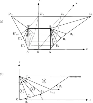
One-Block Mechanism M1
A simple failure mechanism for a rectangular vertical wall is shown diagrammatically in Fig. 1(a). This mechanism is an extension into three dimensions of the 2D well-known Cou-lomb mechanism. The horizontal movement of the wall
AA⬘BB⬘ is accommodated by movement of the material AA⬘BB⬘DD⬘. The Cartesian coordinate system is selected so
that the plane of symmetry coincides with z = 0. Fig. 1(b) shows the vertical section through xOy.
As shown in Fig. 1(a), the M1 mechanism is composed of a single rigid block AA⬘BB⬘DD⬘ bounded by the vertical plane
AA⬘BB⬘, the lower plane AA⬘DD⬘, and the lateral planes ABD
and A⬘B⬘D⬘; it outcrops on the ground surface by the trape-zoidal area BB⬘DD⬘. This mechanism is defined by a single angular parameter1, the dihedral angle between the
horizon-tal plan and the lower plan AA⬘DD⬘.
As in the case of the 2D analysis, the soil mass AA⬘BB⬘DD⬘ moves with velocity V1inclined at an angle of 1⫹ to the
horizontal direction (Fig. 2); the wall moves with velocity V0
and V0,1representing the relative velocity at the soil-structure
interface. All of these velocities are parallel to the vertical symmetrical plane xOy. Note that the velocity V1should also
make an angle with the lateral plane ABD (respectively,
A⬘B⬘D⬘) in order to respect the normality condition. This
im-poses that the angle between the vector V1and its orthogonal
projection on the lateral plane ABD (respectively, A⬘B⬘D⬘) must be equal to . This condition yields the orientation of the lateral planes ABD and A⬘B⬘D⬘ for a given inclination 1
of the lower plane AA⬘DD⬘. It can be shown that the dihedral angle1[cf. Fig. 1(a)] between the lateral plane ABD
(respec-tively, A⬘B⬘D⬘) and the vertical plane xOy can be expressed as
sin
tan =1 2 2 (3)
cos ⫺ sin ( ⫹ )
兹 1
where 1 僆 ]0, /2 ⫺ 2[. The condition 1 < /2 ⫺ 2
ensures that the lateral planes are at maximum in the plane of the wall.
Multiblock Mechanism Mn
A better upper-bound solution would require a more elab-orate failure mechanism Mn [cf. Fig. 3(a)] composed of n rigid blocks. Note that in Fig. 3(a) only five blocks are shown; how-ever, the formulation is applicable to any number of blocks. In this improved mechanism, the horizontal movement of the wall AA⬘BB⬘ is accommodated by movement of n rigid blocks. Fig. 3(b) shows the vertical section through xOy.
TABLE 2. Values of Kpqand Corresponding Geometrical Parameters (M1 Mechanism) (deg) (1) b/h = 0.25 Kpq (2) 1 (3) AGS/bh (4) b/h = 1 Kpq (5) 1 (6) AGS/bh (7) b/h = 10 Kpq (8) 1 (9) AGS/bh (10) 15 9.03 32.76 5.60 4.12 30.36 2.86 2.58 26.14 2.19 20 20.39 27.14 10.80 7.83 25.79 4.48 3.98 22.51 2.72 25 51.63 21.72 22.24 17.25 21.04 7.79 6.81 18.72 3.58 30 160.18 16.39 52.08 47.86 16.09 15.47 13.99 14.68 5.26 35 736.18 11.04 159.28 201.78 10.95 44.18 41.21 10.31 9.76 40 9,108.49 5.60 977.12 2,348.34 5.59 252.79 319.89 5.45 35.58 45 — — — — — — — — —
TABLE 1. Values of Kp␥and Corresponding Geometrical Parameters (M1 Mechanism) (deg) (1) b/h = 0.25 Kp␥ (2) 1 (3) vol/bh2 (4) b/h = 1 Kp␥ (5) 1 (6) vol/bh2 (7) b/h = 10 Kp␥ (8) 1 (9) vol/bh2 (10) 15 6.86 32.31 2.16 3.56 29.46 1.29 2.52 25.77 1.09 20 14.82 26.86 4.00 6.42 25.21 1.90 3.83 22.15 1.33 25 36.36 21.59 7.92 13.41 20.70 3.10 6.41 18.38 1.72 30 110.27 16.33 18.00 35.36 15.93 5.98 12.71 14.40 2.44 35 498.68 11.02 54.04 142.38 10.89 15.70 35.20 10.13 4.26 40 6,103.99 5.60 327.60 1,597.19 5.58 86.16 244.60 5.40 13.79 45 — — — — — — — — —
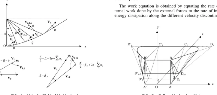
FIG. 5. Failure Mechanism Mnt FIG. 4. Velocity Field of Mn Mechanism
adjacent to the vertical wall and is bounded by the radial plane
the lower plane and the lateral planes
BB⬘D D⬘,1 1 AA⬘D D⬘,1 1
ABD1 andA⬘B⬘D⬘.1 An intermediate block i is limited by two radial planes BB⬘D D⬘i⫺1 i⫺1 and BB⬘D D⬘,i i the lower plane
and the lateral planes BDi⫺1Di and
Di⫺1D⬘ D D⬘,i⫺1 i i B⬘D⬘ D⬘.i⫺1 i
The last block outcrops on the ground surface by a trapezoidal areaBB⬘D D⬘.n n This mechanism is defined by 2n⫺ 1 angular parameters␣i (i = 1, . . . , n ⫺ 1) and i (i = 1, . . . , n) [cf.
Fig. 3(b)].
As shown in Fig. 4, the block velocities Vi and the
inter-block velocitiesVi⫺1,i are parallel to the vertical symmetrical plane xOy. The kinematics of the first block adjacent to the wall is similar to that of the M1 mechanism. For the remaining blocks, the orientation of the lateral plane BDi⫺1Di (respec-tively,B⬘D⬘ D⬘)i⫺1 i is defined by the dihedral anglei between
the planeBB⬘D D⬘i⫺1 i⫺1 and the lateral planeBDi⫺1Di (respec-tively,B⬘D⬘ D⬘).i⫺1 i This angle is determined by orthogonal pro-jection of vector Vi (cf. Fig. 4) on planes BB⬘D D⬘i⫺1 i⫺1 and
(respectively, The calculation details are
BDi⫺1Di B⬘D⬘ D⬘).i⫺1 i
given in Regenass (1999). As for the M1 mechanism,1</
2 ⫺ 2. However, the condition 1 > 0 does not hold in the
present mechanism.
Truncated Multiblock Mechanism Mnt
Further improvement in the upper-bound solution may be obtained by a volume reduction of the final block in the Mn mechanism. In this improved mechanism (cf. Fig. 5), the lower plane and the lateral planes of the last block of the Mn mech-anism are truncated by two portions of right circular cones with vertices at Dn⫺1 and D⬘ ,n⫺1 respectively. The right (re-spectively, left) cone is tangent to the lateral plane BDn⫺1Dn
(respectively,B⬘D⬘ D⬘)n⫺1 n and the lower planeD Dn ⬘Dn n⫺1D⬘ .n⫺1 These cones have axes collinear with the velocity Vn of the
last block. They are characterized by an opening angle equal to 2 in order to satisfy the normality condition for an asso-ciated flow rule Coulomb material. The present mechanism is kinematically admissible because it verifies all of the kine-matical and velocity boundary conditions. The velocity ho-dographs of this mechanism are identical to the ones of the
Mn mechanism. Work Equation
The work equation is obtained by equating the rate of ex-ternal work done by the exex-ternal forces to the rate of inex-ternal energy dissipation along the different velocity discontinuities.
TABLE 3. Values of Kpcand Corresponding Geometrical Parameters (M1 Mechanism) (deg) (1) b/h = 0.25 Kpc (2) 1 (3) Adis/bh (4) b/h = 1 Kpc (5) 1 (6) Adis/bh (7) b/h = 10 Kpc (8) 1 (9) Adis/bh (10) 15 29.84 32.76 14.38 11.50 30.36 6.15 5.78 26.14 3.66 20 53.09 27.14 22.17 18.59 25.79 8.35 8.01 22.51 4.21 25 108.36 21.72 37.70 34.63 21.04 12.62 12.25 18.72 5.14 30 275.44 16.39 75.03 80.90 16.09 22.62 22.24 14.68 6.97 35 1,049.62 11.04 199.69 286.43 10.95 55.14 57.11 10.31 11.87 40 10,853.5 5.60 1,086.06 2,797.09 5.59 280.84 379.68 5.45 39.36 45 — — — — — — — — —
TABLE 4. Ratios Kp␥(3D)/Kp␥(2D) for␦/ ⴝ1 from M1
Mecha-nism (deg) (1) Kp␥(3D)/Kp␥(2D) b/h = 0.25 (2) b/h = 1 (3) b/h = 10 (4) 20 4.20 1.82 1.09 30 10.92 3.50 1.26 40 65.93 17.25 2.64
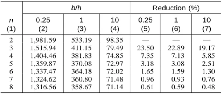
TABLE 5. Kp␥versus Number of Rigid Blocks n from Mn
Mech-anism ( ⴝ45ⴗ;␦/ ⴝ1; and b/hⴝ0.25, 1, and 10) n (1) b/h 0.25 (2) 1 (3) 10 (4) Reduction (%) 0.25 (5) 1 (6) 10 (7) 2 1,981.59 533.19 98.35 — — — 3 1,515.94 411.15 79.49 23.50 22.89 19.17 4 1,404.46 381.83 74.85 7.35 7.13 5.85 5 1,359.87 370.08 72.97 3.18 3.08 2.51 6 1,337.47 364.18 72.02 1.65 1.59 1.30 7 1,324.62 360.80 71.48 0.96 0.93 0.76 8 1,316.56 358.67 71.14 0.61 0.59 0.48
FIG. 6. Comparison of Kp␥and Kpqbetween M1 and Mn
Mech-anisms (␦/ ⴝ1)
The external forces contributing to the rate of external work consist of the passive earth force Pp, the weight of the soil
mass in motion, and the surcharge q on the ground surface. The total rate of external work is given by
˙ ˙ ˙ ˙ W = WPp⫹ W ⫹ W␥ q (4) where ˙ WPp= P cosp ␦ cos( ⫹ )V1 1 (5) n ˙ W =␥ ⫺␥
冘
vol sin(i  ⫹ )Vi i (6) i =1 ˙ Wq⫺ qA sin( ⫹ )VGS n n (7)where voli= volume of block i; and AGS = area of the failure
mechanism at the ground surface.
Energy is dissipated at the soil-wall interface, at the lower and lateral planes between the material at rest and the material in motion, at the radial plane(s) separating the rigid block(s), and at the conical surfaces between the lateral and the lower planes in the Mnt mechanism. The total rate of energy dissi-pation is given by ˙ ˙ ˙ D = Dw⫹ Dlow⫹lat⫹rad⫹con (8) where ˙ D = (P sinw p ␦ ⫹ P )Va 0,1 (9) ˙ Dlow⫹lat⫹rad⫹con n n⫺1
= c cos V
冋 冘
i (Alowi⫹ A ) ⫹ V A ⫹ Vlati n con i⫺1,i冘 册
Aradii =1 i =1 (10)
By equating the total rate of external work to the total rate of energy dissipation along the different velocity discontinui-ties, one obtains
2 h
P = Kp p␥⭈␥⭈ ⭈b ⫹ K ⭈c⭈h⭈b ⫹ K ⭈q⭈h⭈bpc pq (11) 2
TABLE 6. Ratios Kp␥(3D)/Kp␥(2D) for␦/ ⴝ1 from Mn Mecha-nism (deg) (1) Kp␥(3D)/Kp␥(2D) b/h = 0.25 (2) b/h = 1 (3) b/h = 10 (4) 20 3.95 1.75 1.08 30 8.33 2.85 1.19 40 20.12 5.79 1.48
TABLE 7. Kp␥ versus Number of Rigid Blocks n from Mnt
Mechanism ( ⴝ45ⴗ;␦/ ⴝ1; and b/hⴝ0.25, 1, and 10) n (1) b/h 0.25 (2) 1 (3) 10 (4) Reduction (%) 0.25 (5) 1 (6) 10 (7) 2 784.56 235.81 69.14 — — — 3 728.41 217.45 61.53 7.16 7.79 11.01 4 717.13 213.71 59.84 1.55 1.72 2.74 5 713.09 212.36 59.22 0.56 0.63 1.04 6 711.21 211.74 58.92 0.26 0.30 0.50 7 710.18 211.39 58.76 0.14 0.16 0.28
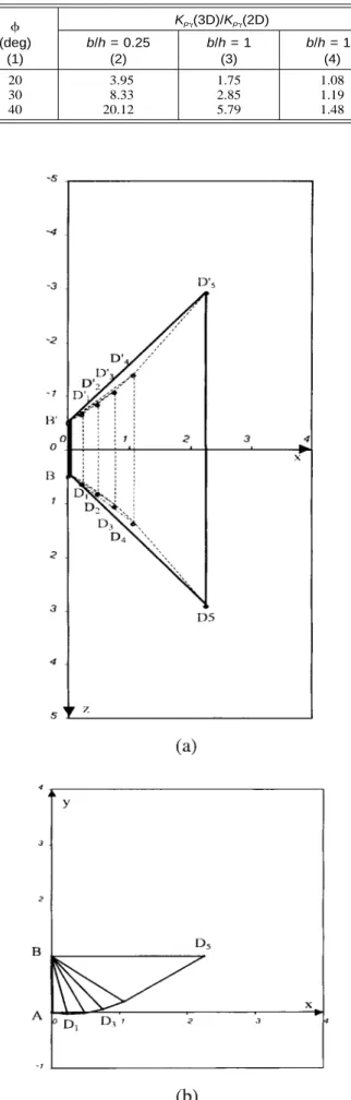
FIG. 7. Traces of Mn Mechanism: (a) Plan View; (b) Vertical Section through xOy ( ⴝ30ⴗ,␦/ ⴝ1, and b/hⴝ1)
where Kp␥, Kpc, and Kpq = passive earth pressure coefficients
due to soil weight, cohesion, and surcharge loading, respec-tively. These coefficients are function of , ␦, and b/h. NUMERICAL RESULTS
The most critical passive earth pressure coefficients can be obtained by a minimization procedure of these coefficients with respect to the angular parameters describing the different failure mechanisms. Three computer programs using the VBA programming language that resides in Microsoft Excel have been written to define the coefficients of passive earth pres-sures as function of the mechanisms’ parameters. The mini-mization procedure is performed using the Solver optimini-mization tool of Microsoft Excel. The method of minimization used is the general reduced gradient method. The programs give the minimal passive earth pressure coefficients and the corre-sponding critical slip surfaces. In the following sections, one first presents the Kp␥, Kpq, and Kpc coefficients obtained from
the three failure mechanisms. Then, in the spirit of the upper-bound approach, the lesser of the three solutions is given in the form of design tables for practical use in geotechnical en-gineering.
Results from M1 Mechanism
Some results from the M1 mechanism are presented in Ta-bles 1 – 3 where the values of Kp␥, Kpq, and Kpc are tabulated
for ranging from 15⬚ to 45⬚, for ␦/ = 1, and for three values of b/h (b/h = 0.25, 1, and 10). The optimum values of the parameter 1 and the corresponding normalized critical
ge-ometry of the potentially sliding mass (i.e., vol/bh2
for Kp␥,
AGS/bh for Kpq and Adis/bh for Kpc) are also listed against the
coefficients of passive earth pressures K where vol = total vol-ume of the soil mass in motion; and Adis = area of velocity
discontinuities.
Note that for = 45⬚, there is no solution since the restric-tive condition concerning angle1 implies that1= 0 in that
particular case. Tables 1 – 3 clearly shows that the passive earth pressure coefficients and the corresponding optimal geometry (i.e., volume or surface) increase with increasing. This in-crease is significant for great values. For instance, for b/h = 1 and␦/ = 1, an increase in the soil internal friction angle from 20⬚ to 25⬚ increases the coefficient Kp␥by a factor of 2.1 and the volume vol/bh2
by 1.6. However, an increase in from 35⬚ to 40⬚ increases Kp␥ by a factor of 11.2 and the volume vol/bh2
by 5.5. Hence, the present mechanism seems to greatly overestimate the passive earth pressure coefficients for great
values.
Of particular interest in Tables 2 and 3 is the same optimal parameter1 obtained from the minimization of both Kpqand
Kpc coefficients. It is also interesting to note that these
coef-ficients are related by the following relationship [cf. theorem of corresponding states of Caquot (Caquot and Ke´risel 1949)]:
SectionthroughxOy( ⴝ 30ⴗ, ␦/ ⴝ 1,andb/h ⴝ 1)
FIG. 9. Traces of Mnt Mechanism: (a) Plan View; (b) Vertical TABLE 8. Ratio Kp␥(3D)/Kp␥(2D) for␦/ ⴝ1 from Mnt
Mecha-nism (deg) (1) Kp␥(3D)/Kp␥(2D) b/h = 0.25 (2) b/h = 1 (3) b/h = 10 (4) 20 3.39 1.64 1.07 30 6.16 2.36 1.15 40 12.08 3.86 1.33
FIG. 8. Comparison of Kp␥and Kpqbetween Mn and Mnt
Mech-anisms (␦/ ⴝ1) 1 Kpq⫺ cos␦ Kpc= (12) tan
Thus, in the following sections, only Kp␥and Kpqcoefficients
will be presented; Kpcmay be computed using (12).
Table 4 presents the ratios Kp␥(3D)/Kp␥(2D) for ranging
from 20⬚ to 40⬚, for ␦/ = 1, and for three values of b/h (b/h = 0.25, 1, and 10).
FIG. 10. Traces in Plan View of Mnt Mechanism for ⴝ20ⴗ, 30ⴗ, 40ⴗ;␦/ ⴝ0 and 1; and b/hⴝ1
FIG. 11. Kp␥versusfor␦/ ⴝ0, 1/2, and 1 when b/hⴝ1 Notice that as the length b/h increases, the ratio Kp␥(3D)/
Kp␥(2D) decreases; that is, the end effect decreases. It should be emphasized that, when 2D problems (i.e., large values of
b/h) are used, the passive earth pressure coefficients predicted
based on the current analysis are identical to those of 2D anal-ysis given by Chen (1975). As shown in Table 4, the end effects are most pronounced for great values. For instance, for b/h = 10, the ratio Kp␥(3D)/Kp␥(2D) is equal to 1.09 when
= 20⬚ and attains 2.64 when = 40⬚.
Results from Mn Mechanism
Table 5 presents the Kp␥ coefficient obtained from the Mn mechanism for various values of n (the number of rigid blocks) when = 45⬚; ␦/ = 1; and b/h = 0.25, 1, and 10. This table shows that the upper-bound solution can be im-proved by increasing the number of rigid blocks. The reduc-tion in the Kp␥value decreases with the n increase (1.59% for
n = 6 and b/h = 1). Hence, all subsequent results are given for n = 5 blocks.
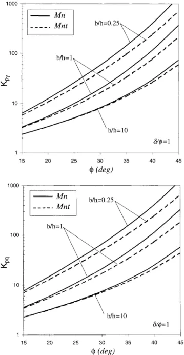
Some results of Kp␥and Kpq obtained from the Mn
mecha-nism are compared to those given by the M1 mechamecha-nism in Fig. 6 for ranging from 15⬚ to 45⬚, for ␦/ = 1, and for three values of b/h (b/h = 0.25, 1, and 10).
As expected, the Mn mechanism gives better results than the M1 mechanism. This may be explained by the fact that the geometry of the Mn mechanism is less restrictive than that of
the M1 mechanism. For instance, when = 40⬚, ␦/ = 1, and
b/h = 1, the improvement of the solution attains 92.8%.
Table 6 presents the ratios Kp␥(3D)/Kp␥(2D) for ranging from 20⬚ to 40⬚, for ␦/ = 1, and for three values of b/h (b/h = 0.25, 1, and 10). This table exhibits trends similar to those
TABLE 9. Kp␥Values for Various Governing Parameters,␦, and b/h b/h (1) (deg) (2) ␦/ 0 (3) 1/3 (4) 1/2 (5) 2/3 (6) 1 (7) 0.25 15 3.633 3.634 3.635 3.636 3.637 20 5.399 5.400 5.401 5.402 5.403 25 7.983 7.984 7.985 7.986 7.987 30 11.886 11.887 11.888 11.889 11.890 35 20.044 20.045 20.046 20.047 20.048 40 50.430 50.431 50.432 50.433 50.434 45 215.455 215.456 215.457 215.458 215.459 0.5 15 2.673 3.062 3.282 3.524 4.054 20 3.726 4.538 5.041 5.629 6.994 25 5.229 6.849 7.963 9.379 12.776 30 7.443 10.604 13.096 16.634 25.085 35 11.984 17.354 22.855 32.487 54.064 40 28.594 40.954 53.74 79.700 131.753 45 114.009 148.475 178.689 224.310 379.494 1 15 2.190 2.490 2.658 2.841 3.191 20 2.887 3.487 3.853 4.279 5.139 25 3.850 5.001 5.779 6.760 8.798 30 5.221 7.391 9.067 11.418 16.273 35 7.954 11.518 15.150 21.308 33.202 40 17.676 25.317 31.218 49.269 77.015 45 63.152 82.517 99.555 125.324 212.364 2 15 1.946 2.189 2.340 2.492 2.737 20 2.466 2.956 3.252 3.593 4.171 25 3.159 4.069 4.677 5.435 6.746 30 4.111 5.777 7.038 8.787 11.764 35 5.939 8.600 11.279 15.683 22.607 40 12.218 17.499 22.962 32.329 49.371 45 37.520 49.289 59.708 75.515 128.306 5 15 1.798 2.022 2.145 2.256 2.451 20 2.211 2.633 2.885 3.133 3.561 25 2.743 3.505 4.006 4.542 5.456 30 3.444 4.801 5.808 6.965 8.948 35 4.73 6.849 8.938 11.519 16.035 40 8.942 12.808 16.806 21.145 32.361 45 21.743 28.869 35.262 45.043 76.983 10 15 1.748 1.962 2.069 2.169 2.352 20 2.125 2.524 2.748 2.954 3.348 25 2.604 3.315 3.770 4.178 5.004 30 3.222 4.473 5.394 6.209 7.958 35 4.327 6.266 8.150 9.870 13.730 40 7.851 11.244 14.754 17.226 26.424 45 16.153 21.665 26.684 34.430 59.215 Strip 15 1.698 1.891 1.987 2.080 2.250 20 2.040 2.393 2.579 2.768 3.127 25 2.464 3.080 3.427 3.794 4.529 30 3.000 4.052 4.692 5.402 6.905 35 3.690 5.484 6.677 8.075 11.242 40 4.599 7.698 9.992 12.863 19.938 45 5.828 11.350 16.019 22.313 39.644
TABLE 10. KpqValues for Various Governing Parameters,␦,
and b/h b/h (1) (deg) (2) ␦/ 0 (3) 1/3 (4) 1/2 (5) 2/3 (6) 1 (7) 0.25 15 4.588 5.315 5.735 6.201 6.983 20 7.068 8.704 9.736 10.960 13.015 25 10.736 14.202 16.635 19.770 24.817 30 16.329 23.415 29.140 37.382 49.352 35 28.104 40.698 53.606 77.039 104.684 40 72.265 103.502 135.815 170.861 243.616 45 221.247 283.828 336.637 412.522 646.788 0.5 15 3.153 3.628 3.900 4.198 4.625 20 4.563 5.583 6.219 6.967 8.057 25 6.606 8.690 10.135 11.984 14.599 30 9.664 13.810 17.113 21.829 27.909 35 16.014 23.190 30.545 43.615 57.371 40 39.512 56.591 74.259 91.492 130.190 45 115.741 148.661 176.444 216.319 338.705 1 15 2.432 2.777 2.972 3.182 3.419 20 3.307 4.014 4.449 4.956 5.543 25 4.540 5.926 6.873 8.073 9.445 30 6.332 8.999 11.084 13.951 17.124 35 9.969 14.436 19.006 25.670 33.627 40 23.136 33.136 43.481 51.724 73.351 45 62.912 80.988 96.248 118.102 184.474 2 15 2.068 2.345 2.499 2.620 2.798 20 2.677 3.223 3.554 3.848 4.256 25 3.505 4.536 5.229 5.902 6.819 30 4.666 6.585 8.055 9.562 11.656 35 6.946 10.059 13.218 16.622 21.638 40 14.947 21.408 26.666 31.723 44.748 45 36.374 47.008 55.993 68.811 107.059 5 15 1.848 2.081 2.185 2.271 2.409 20 2.296 2.741 2.969 3.148 3.453 25 2.882 3.694 4.176 4.533 5.189 30 3.666 5.127 6.147 6.865 8.277 35 5.133 7.433 9.615 11.077 14.269 40 10.034 13.923 16.376 19.515 27.268 45 20.194 26.327 31.524 38.875 60.019 10 15 1.773 1.986 2.072 2.152 2.274 20 2.168 2.577 2.746 2.906 3.173 25 2.673 3.410 3.748 4.060 4.620 30 3.333 4.637 5.316 5.924 7.100 35 4.528 6.558 7.951 9.155 11.708 40 8.263 10.838 12.821 15.303 21.219 45 14.571 19.177 23.101 28.599 43.854 Strip 15 1.698 1.878 1.956 2.027 2.133 20 2.040 2.365 2.516 2.655 2.881 25 2.464 3.026 3.302 3.565 4.021 30 3.000 3.947 4.443 4.937 5.846 35 3.690 5.278 6.173 7.105 8.949 40 4.599 7.286 8.928 10.750 14.643 45 5.828 10.486 13.657 17.367 26.168
observed in Table 4. On the other hand, for b/h = 10 and = 40⬚, the present value of the ratio Kp␥(3D)/Kp␥(2D) = 1.48 may
be compared with the previous value of Kp␥(3D)/Kp␥(2D) = 2.64 obtained from the M1 mechanism. One may conclude that the present mechanism gives better predictions of the 3D effect.
Fig. 7 shows the plan view and the cross section through
xOy of the Mn mechanism as obtained from the minimization
of Kp␥when = 30⬚, ␦/ = 1, and b/h = 1.
It can be observed that the volume of the last block is significant in comparison to the remaining
BD D B4 5 ⬘D⬘D⬘4 5
blocks.
Results from Mnt Mechanism
Table 7 presents the Kp␥coefficient obtained from the Mnt mechanism for various values of n when = 45⬚; ␦/ = 1; and b/h = 0.25, 1, and 10.
The reduction in the Kp␥ value is equal to 7.8% when n = 3 and attains 0.3% when n = 6 for b/h = 1. One may conclude
that the present mechanism rapidly converges to the optimal solution. Hence, in the following section, only five rigid blocks are used, which means that the minimization procedure is made with respect to nine angular parameters.
The results of Kp␥and Kpqobtained from the present
mech-anism are compared to those given by the Mn mechmech-anism in Fig. 8.
As expected, the Mnt mechanism gives better results than the Mn mechanism. For instance, when = 45⬚, ␦/ = 1, and
b/h = 1, the improvement of the solution attains 42.6%.
Table 8 presents the ratios Kp␥(3D)/Kp␥(2D) for ranging from 20⬚ to 40⬚, for ␦/ = 1, and for three values of b/h (b/h = 0.25, 1, and 10).
As shown in Table 8, the Mnt mechanism gives better pre-dictions of the 3D effect because, for the same case considered in the preceding sections (i.e., b/h = 10 and = 40⬚), the present value of the ratio Kp␥(3D)/Kp␥(2D) = 1.33 is smaller than the one obtained from the Mn mechanism (cf. Table 6).
FIG. 13. Comparison with Blum (1932) for: (a) ⴝ15ⴗ; (b)= 35ⴗ
FIG. 12. Blum’s Failure Mechanism
xOy of the Mnt mechanism as obtained from the minimization
of Kp␥when = 30⬚, ␦/ = 1, and b/h = 1.
In the plan view, the Mnt mechanism is bounded by the traces of the lateral planes BM and B⬘M⬘, the trace of the lower plane NN⬘, and the traces of the conical sectors MN and M⬘N⬘. As is the case with Mn, the present failure mechanism mobi-lizes a great volume for the last block.
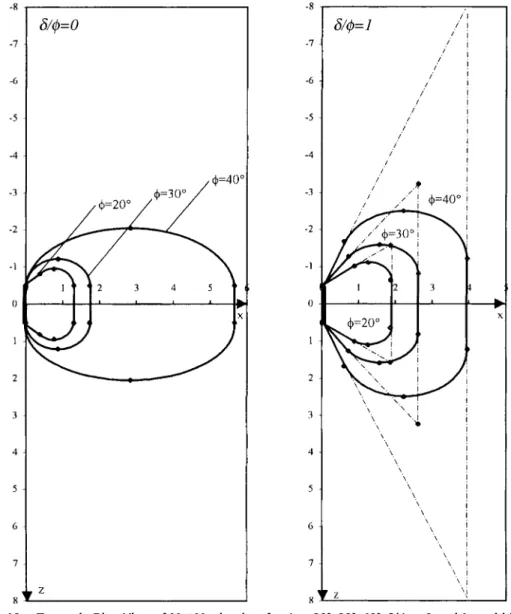
Fig. 10 shows the traces in the plan view of the Mnt mech-anism for = 20⬚, 30⬚, and 40⬚ when ␦/ = 0 and 1 and b/h = 1.
For ␦/ = 0, one can observe a significant change in the failure surface between = 30⬚ and 40⬚. This can be explained by the fact that, for a smooth wall and when < 30⬚, the critical failure mechanism as given by the numerical minimi-zation is obtained for n = 1 (i.e., one-block truncated mecha-nism). The five-block mechanism is of interest only for great
and ␦ values.
Finally, it should be mentioned that the trace of the present failure mechanism in plan view is smooth as observed exper-imentally by Meksaouine (1993).
Discussion of Results
As shown before, the Mnt mechanism gives the least upper-bound solution to the 3D passive earth pressure problem.
Fig. 11 shows the variation of Kp␥with for ␦/ = 0, 1/2, and 1 when b/h = 1.
For a rough wall (␦/ > 2/3), the critical Kp␥ values are obtained with the maximal allowable number of blocks (i.e., five blocks in the present case). However, when␦/ < 2/3 and
< 40⬚, the critical failure mechanism as obtained from the
numerical minimization is reduced to the one-block truncated mechanism. On the other hand, it should be mentioned that for b/h > 7 the maximal number of blocks is needed to obtain the optimal solution. This is to be expected because, in that case (i.e., 2D analysis), the one-block mechanism greatly over-estimates the passive earth pressure coefficients for great and␦ values.
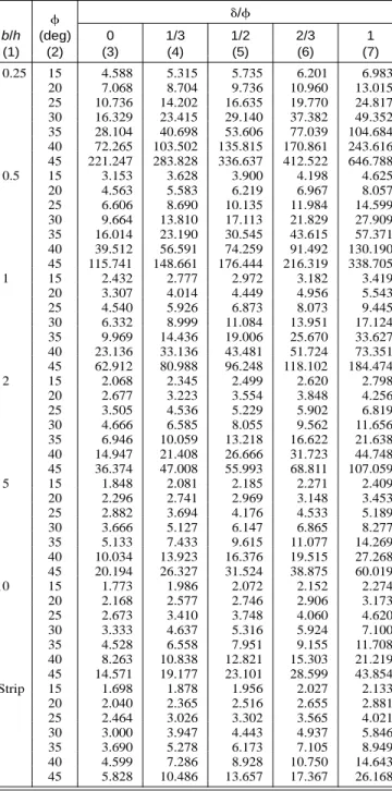
Finally, extensive numerical results of Kp␥ and Kpq as
ob-tained from the Mnt mechanism for various governing param-eters are given in Tables 9 and 10 for practical use in geo-technical engineering.
Comparison with Existing Solutions
Although the 2D passive earth pressure problem has been widely treated in the literature using different approaches, the 3D passive earth pressure problem has received little attention apart from the work of Blum (1932) using the limit-equilib-rium method. As shown in Fig. 12, Blum’s mechanism is an extension into three dimensions of the traditional one-block Coulomb mechanism in which the frictional forces at the
lat-eral planes are neglected. According to Blum (1932), the 3D passive earth force is given by
3
1 2 2 h 2
P =p ␥h b tan
冉 冊
⫹ ⫹ ␥ tan冉 冊
⫹ (13)2 4 2 6 4 2
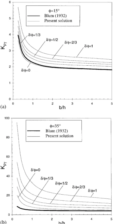
Figs. 13(a and b) show the comparison between the present results and those given by Blum (1932) for = 15⬚ and 35⬚; for ␦/ = 0, 1/3, 1/2, 2/3, and 1; and for different values of
b/h.
These figures clearly show that Blum’s solutions are in good agreement with the present solutions only for loose sand and a smooth wall. However, for dense sand and rough wall, Blum’s solutions greatly underestimate the passive earth pres-sure coefficients. This difference may be explained by the fact that the lower slip surface in Blum’s mechanism is assumed to be planar. Furthermore, Blum made an a priori assumption
concerning the length of DC at the ground level (cf. Fig. 12). Finally, Blum neglected the frictional forces on the lateral planes AED and BFC.
CONCLUSIONS
Similar to the 2D analysis, the one-block 3D failure mech-anism M1 greatly overestimates the passive earth pressures for great and ␦ values.
The multiblock mechanism Mn improves the results given by the M1 mechanism due to the flexibility of this mechanism especially for great values of and ␦. It gives better predic-tions of the 3D effect. However, the trace of the failure mech-anism in the plan view is not as smooth as observed experi-mentally by Meksaouine (1993).
Finally, the truncated multiblock mechanism is more effi-cient than the Mn mechanism because it gives smaller upper-bound solutions and leads to a critical slip surface in the plan view that is similar to that observed experimentally.
The numerical results have shown that the truncated mul-tiblock mechanism is reduced to the truncated one-block mechanism for␦/ < 2/3 and < 40⬚; otherwise, the truncated five-block mechanism is needed to obtain the optimal upper-bound solutions.
The comparison of the results obtained from the Mnt mech-anism with those given by the classical Blum solutions has shown that this author greatly underestimates the passive earth pressure coefficients for a rough wall and a dense sand.
Finally, numerical results based on the Mnt mechanism for various governing parameters are given for practical use.
APPENDIX. REFERENCES
Blum, H. (1932). ‘‘Wirtschaftliche Dalbenformen und deren Berech-nung.’’ Bautechnik, 10(5), 122–135 (in German).
Caquot, A., and Ke´risel, J. (1949). Traite´ de me´canique des sols, Gau-thier-Villars, Paris (in French).
Chen, W. F. (1975). Limit analysis and soil plasticity, Elsevier Science, Amsterdam.
Chen, W. F., and Rosenfarb, J. L. (1973). ‘‘Limit analysis solutions of earth pressure problems.’’ Soils and Found., Tokyo, 13(4), 45–60. Collins, I. F. (1969). ‘‘The upper-bound theorem for rigid/plastic solids
to include Coulomb friction.’’ J. Mech. Phys. Solids, 17, 323–338. Collins, I. F. (1973). ‘‘A note on the interpretation of Coulomb’s analysis
of the thrust on a rough retaining wall in terms of the limit theorems of plasticity theory.’’ Ge´otechnique, London, 24(1), 106–108.
Coulomb, C. A. (1773). ‘‘Sur une application des re`gles de maximis et minimis a` quelques proble`mes de statique relatifs a` l’architecture.’’ Acad. R. Sci. Me´m. Math. Phys., 7, 343–382 (in French).
Drescher, A., and Detournay, E. (1993). ‘‘Limit load in translational fail-ure mechanisms for associative and non-associative materials.’’ Ge´o-technique, London, 43(3), 443–456.
Lee, I. K., and Herington, J. R. (1972). ‘‘A theoretical study of the pres-sures acting on a rigid wall by a sloping earth on rockfill.’’ Ge´otech-nique, London, 22(1), 1–26.
Lysmer, J. (1970). ‘‘Limit analysis of plane problems in soil mechanics.’’ J. Soil Mech. and Found. Div., ASCE, 96(4), 1311–1334.
Meksaouine, M. (1993). ‘‘Etude expe´rimentale et the´orique de la pousse´e passive sur pieux rigides.’’ PhD thesis, Institut National des Sciences Applique´es de Lyon, Lyon, France (in French).
Michalowski, R. L. (1999). ‘‘Closure on ‘Stability of uniformly reinforced slopes.’ ’’ J. Geotech. and Geoenvir. Engrg., ASCE, 125(1), 81–86. Michalowski, R. L., and Shi, L. (1995). ‘‘Bearing capacity of footings
over two-layer foundation soils.’’ J. Geotech. Engrg., ASCE, 121(5), 421–428.
Michalowski, R. L., and Shi, L. (1996). ‘‘Closure on ‘Bearing capacity of footings over two-layer foundation soils.’ ’’ J. Geotech. Engrg., ASCE, 122(8), 701–703.
Mroz, Z., and Drescher, A. (1969). ‘‘Limit plasticity approach to some cases of flow of bulk solids.’’ J. Engrg. Ind. Trans. Am. Soc. Mech. Engrs., 91, 357–364.
Rahardjo, H., and Fredlund, D. G. (1984). ‘‘General limit equilibrium method for lateral earth force.’’ Can. Geotech. J., Ottawa, 21(1), 166–175.
Regenass, P. (1999). ‘‘Application de la me´thode cine´matique de l’analyse limite au calcul de la bute´e tridimensionnelle et de la charge limite de plaques d’ancrage superficielles.’’ PhD thesis, Universite´ Louis Pasteur, Strasbourg, France (in French).
Shields, D. H., and Tolunay, A. Z. (1972). ‘‘Passive pressure coefficients for sand by the Terzaghi and Peck method.’’ Can. Geotech. J., Ottawa, 9(4), 501–503.
Shields, D. H., and Tolunay, A. Z. (1973). ‘‘Passive pressure coefficients by methods of slices.’’ J. Soil Mech. and Found. Div., ASCE, 99(12), 1043–1053.
Sokolovski, V. V. (1960). Static of granular media, Butterworth’s, Lon-don.
Soubra, A.-H. (2000). ‘‘Static and seismic passive earth pressure coeffi-cients on rigid retaining structures.’’ Can. Geotech. J., Ottawa, 37(2), in press.
Soubra, A.-H., Kastner, R., and Benmansour, A. (1999). ‘‘Passive earth pressures in the presence of hydraulic gradients.’’ Ge´otechnique, Lon-don, 49(3), 319–330.
Terzaghi, K. (1943). Theoretical soil mechanics, Wiley, New York. Zakerzadeh, N., Fredlund, D. G., and Pufahl, D. E. (1999). ‘‘Interslice
force functions for computing active and passive earth force.’’ Can. Geotech. J., Ottawa, 36(6), 1015–1029.
![Dissociative ionization of neon clusters Ne[sub n], n=3 to 14: A realistic multisurface dynamical study](data:image/gif;base64,R0lGODlhAQABAIAAAP///wAAACH5BAEAAAAALAAAAAABAAEAAAICRAEAOw==)