Non-incremental strategies for simulating thermomechanical models with uncertainty

HAL Id: hal-02424650

https://hal.archives-ouvertes.fr/hal-02424650

Submitted on 27 Dec 2019

HAL is a multi-disciplinary open access

archive for the deposit and dissemination of

sci-entific research documents, whether they are

pub-lished or not. The documents may come from

teaching and research institutions in France or

abroad, or from public or private research centers.

L’archive ouverte pluridisciplinaire HAL, est

destinée au dépôt et à la diffusion de documents

scientifiques de niveau recherche, publiés ou non,

émanant des établissements d’enseignement et de

recherche français ou étrangers, des laboratoires

publics ou privés.

Non-incremental strategies for simulating

thermomechanical models with uncertainty

Francisco Chinesta, Etienne Prulière, Amine Ammar, Elías Cueto

To cite this version:

Francisco Chinesta, Etienne Prulière, Amine Ammar, Elías Cueto. Non-incremental strategies for

simulating thermomechanical models with uncertainty. International Journal of Material Forming,

Springer Verlag, 2009, 2 (S1), pp.563-566. �10.1007/s12289-009-0422-z�. �hal-02424650�

____________________

* Corresponding author: 1 rue de la Noë, BP 92101, 44321 Nantes - France, (33) 2 40 37 16 00, Etienne.Pruliere@ec-nantes.fr

NON-INCREMENTAL STRATEGIES FOR SIMULATING

THERMOMECHANICAL MODELS WITH UNCERTAINTY

F. Chinesta

1

, E. Prulière

1*

, A. Ammar

2

, E. Cueto

3

1

_{Ecole Centrale de Nantes, EADS Corporate International Chair, Nantes, France}

2

_{Université Joseph Fourier, Laboratoire de Rhéologie, UMR CNRS, Grenoble, France}

3

_{I3A, Universidad de Zaragoza, Spain.}

ABSTRACT: Description of complex materials involves numerous computational challenges. Thus, the analysis of transient models needs for intensive computation. In some of our former works we proposed a technique based on the separated representation of the unknown field able to circumvent the curse of dimensionality in the treatment of highly multidimensional models. In this work, we are addressing the challenge related to the transient behaviour. For this purpose we propose a separated representation of transient models leading to a non-incremental strategy, allowing to impressive CPU time savings. The use of separated representations allows computing the solution of transient parametric models (the parameters are assumed as additional coordinates). The parameters include thermal coefficients but also thermal sources and/or initial conditions. The resulting curse of dimensionality is circumvented by using the separated representation that implies a complexity that scales linearly with the dimension of the space.

KEYWORDS: Reduced representation, Parametric model, Multi-dimensional models, Separated representation.

1 INTRODUCTION

The complexity of coupled thermomechanical models defined in domains involving very fine space and time meshes induce computational issues. On the other hand, some times the parametric nature of such models (because of different uncertainties) induces additional difficulties. The use of explicit incremental methods is restricted to very short time steps because of the stability requirements. On the other hand, implicit incremental methods need the solution of a linear system at each time step in the general non-linear case. In any case, the treatment of parametric models requires the solutions of many direct models. To circumvent these difficulties one could use reduced approximation bases within the incremental framework. Another possibility lies in the use of an alternative non-incremental technique. This work explores the use of a particular non-incremental technique based on the separated representation of the unknown field.

2 SOLVING PROBLEMS WITH

UNCERTAINTY

Let’s consider the general heat equation:

( , )

_{( , )}

_{( , )}

u t

_k

_{u t}

_{f t}

t

∂

∂



∂



−

_

_

=

∂

∂



∂



x

_x

_x

x

x

(1)

with the following initial condition:

0

( 0, )

( )

u t

=

x u x

=

(2)

where u is the temperature field and k the thermal conductivity. In general the thermal conductivity depends on the temperature, but in what follows we are assuming that the conductivity is constant but unknown. 2.1 ON A SEPARATED REPRESENTATION To solve multidimensional problems with a low calculation cost, an efficient method has been recently developed. This technique was successfully applied for treating some multi-dimensional models encountered in the kinetic theory description of complex fluids [1] [2] [3] and for treating high resolution thermal homogenization [5]. For the sake of simplicity the method is described here in the 1D transient case defined by: 2 2

( , )

_{( , ) 0}

u t x

_k

u t x

t

x

∂

∂

−

=

∂

∂

(3)

For that purpose let us consider the weak formulation of the heat equation:

2 * 2

0

u

u

u

k

t

x

Ω



∂

∂



−

=





∂

∂





∫

(4)

where

Ω =

]

0,

t

_max

] ]

×

x

_min

,

x

_max

[

= Ω ×Ω

_{t x}

The main idea is the assumption that the solution can be written in the following separated form:

0 1

( , )

N i

( ) ( )

i i

u t x

T t X x u

=

≈

∑

+

(5)

The introduction of u0 in the previous expression enables

to enforce an homogeneous initial condition, i.e.:

( 0) 0

i

T t

=

=

∀ ≤

i N

(6)

Building-up such a solution needs an iterative procedure. At the iteration n we assume that the function Ti and Xi

are known

∀ ≤

i n

. Then we are looking for:

0 1

( ) ( )

( ) ( )

n i i i

u

T t X x R t S x u

=

≈

∑

+

+

(7)

where R and S have to be determined. We assume the weighting field:

* *

_{( ) ( )}

_{( ) ( )}

*

u

=

R t S x R t S x

+

(8) Thus, the resulting weak formulation writes:

(

)

2 2 2 * * 0 2 2 2 1 0 n i i i i i dT d X dR d S d u R S RS X kT S kR k d dt dx dt dx dx Ω ₌     + _{ } − _+ − − _ Ω =   ∑  ∫ (9)

that defines a non-linear problem which needs an iterative process to be solved. An alternate directions strategy has given excellent results in our former studies [1],[2],[6]. This method is performed in two steps: Step 1: R being known, we are looking for S. Step 2: S being known, we are looking for R.

Starting with an arbitrary tentative function R, we perform step 1 and then step 2, and again both steps until reaching convergence. Only step 1 will be described now, step 2 being very similar. Thus, R is assumed known and then

R =

*

0

. It results:

2 * * 2 1 2 2 * 2 * * 0 2 2 0 t x t x t x t x t x n i i i i i dT d X R S X kRT S dt dx d u dR d S R S S kR S kR S dt dx dx Ω Ω Ω Ω = Ω Ω Ω Ω Ω Ω   − +     − − =

∑ ∫

∫

∫

∫

∫

∫

∫

∫

∫

∫

(10) The integrals on

Ω

_t can be computed numerically. We denote by

α

_i,

β

_i and

γ

these integrals, leading to:

2 2 * * * 0 0 0 2 2 2 * * 2 1 x x x x x n i i i i i

d u

d S

S S

S

S

dx

dx

d X

S X

S

dx

α

β

γ

α

β

Ω Ω Ω Ω Ω =

−

=





−

_

−

_





∫

∫

∫

∑ ∫

∫

(11)

This is a 1D steady-state weak formulation (3D in the general case) which can be solved for instance with the

finite elements method, but if we extract the strong form, then it could be solved using any discretization technique.

2.2 ADRESSING PARAMETRIC MODELS 2.2.1 Introducing new coordinates

In this section, we consider a model in which there is an uncertainty on one or many parameters. For illustration purposes, we want to solve the heat equation where the thermal conductivity k is a badly known, but constant, parameter. A way to overcome this difficulty is to take k as a new coordinate belonging to the uncertainty interval. The transient solution for a particular value of the conductivity can then be computed by restricting the general solution to each particular value of this extra-coordinate. Obviously, the price to be paid is the increase of the model dimensionality. However, this is not a serious issue when one proceeds within the separated representation framework just described. The solution is now assumed as:

0 1

( , , )

N i

( ) ( ) ( )

i i i

u t x k

T t X x K k u

=

≈

∑

+

(12)

The iterative method described in the previous section is then used to compute the solution.

2.2.2 Results

We consider the heat problem in the domain

] [

1,1

x

Ω = −

with, for the sake of simplicity, homogeneous essential boundary conditions. The initial condition is:

u x

₀

( ) 1

= −

x

2 and we want to compute the temperature until tmax=0.5s. and for

1

≤ ≤

k

10

.

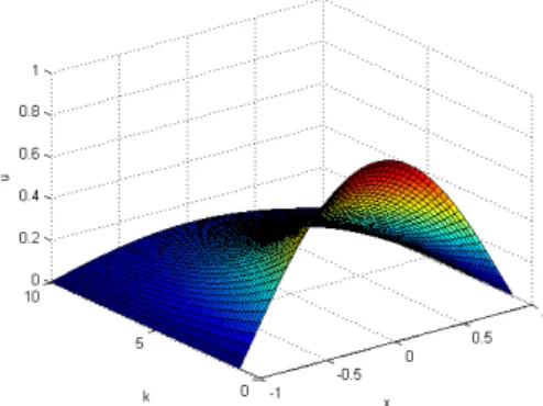
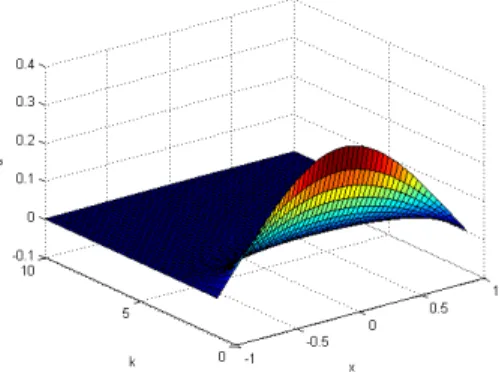
The temperature field versus the thermal conductivity is depict in Figure 1 at time t=0.1s. and in Figure 2 at time

t=0.5s. A reduced number of sums allow computing the

solution with a reasonable accuracy. Obviously, the accuracy can be improved by using more sums in the separated approximation. In the limit case, the computed solution approaches the one computed by using the standard finite element method.

Figure 1: Temperature versus thermal conductivity and

Figure 2: Temperature versus thermal conductivity and

position at time t=0.5s.

3 TOWARDS FURTHER REDUCTION

3.1 REDUCED SEPARATED REPRESENTATION Though the separated representation allows considerable time savings, one could envisage additional CPU time savings. For instance the heat equation defined in large 2D or 3D domains needs the solution of large linear systems at step 1 of the iterative strategy presented above. We analyze the solution of the space step:

1

( )

nx i

( )

i i

S x

B x s

=

=

∑

(13)

where Bi are the basis functions whose number is nx and si are the weights associated with these basis functions.

With this approximation, the virtual field yields:

* * 1

( )

nx i

( )

i i

S x

B x s

=

=

∑

(14)

Introducing these notations in Eq. (11) it results:

(

)

2 * * 0 0 2 , 1 , 1 2 * 0 2 1 2 * 2 1 1 x x x x x x x x x n n j i i j j i i j i j i j n i i i n n j i j i j j i i j

d B

s

B B s

s

B

s

dx

d u

s

B

dx

d X

s

B X

B

dx

α

β

γ

α

β

Ω Ω = = Ω = Ω Ω = =





−



_



_

=









=

_

_

−













−





_

−



_















∑

_∫

∑

_∫

∑ ∫

∑ ∑ ∫

∫

(15)

that leads to the linear system:

=

Ms V

(16)

where M is a

n n

_x

×

_x matrix. If nx is smaller than the

number of nodes distributed in the space, then significant CPU time savings can be accomplished.

Remark: Such an approximation may also be performed on the time space for the function R(t).

3.2 BUILDING-UP THE APPROXIMATION The main remaining question is how to build-up an optimal approximation basis. A solution is to build the basis functions by invoking the proper orthogonal decomposition as was performed in [4]. The main issue is the necessity to perform some previous simulations. We have opted for an “a priori” strategy. The idea is to check (at each iteration of the computation of S (respect.

R)) if the basis needs to be enriched, and if that is the

case, to propose an optimal enrichment. 3.2.1 Checking the accuracy of the basis

We assume that the basis functions are known for

x

i n

≤

. The computation of S requires the resolution of Eq. (15). The weights si in that basis are assumed known.

To check the accuracy of the basis, we compute the residual function that can be easily derived from Eq. (15): 2 0 0 2 1 1 2 2 0 2 2 1

Res

nx nx i i i i i i n j j j j j

d B

B s

s

dx

d X

d u

_X

dx

dx

α

β

γ

α

β

= = =

=

−

−





+



_

−



_





∑

∑

∑

(17)

If the residual norm is greater than a given small enough value: 2

Res

Res

x

ε

S

Ω

=

_∫

>

(18)

the basis must be enriched. On the contrary, if the norm of the residual is small enough, we continue to the next iteration keeping the same reduced basis.

3.2.2 Enrichment of the basis

The main aim is to define the enriched function

B′

and the corresponding weight

s′

in order to cancel the residual. From Eq. (17) we can write:

2 2 0 0 2 2 1 1 2 2 0 2 2 1

0

x x n n i i i i i i n j j j j j

d B

d B

B s B s

s

s

dx

dx

d X

d u

_X

dx

dx

α

β

γ

α

β

= = =







′ 

′ ′

′

+

−

+





















−

+



_

−



_

=





∑

∑

∑

(19)

that taking into account Eq. (17) leads to:

2 0 0 2

Res

d B

B s

s

dx

α

′ ′

−

β

′

′

= −

(20) which is an ordinary differential equation, that could be solved under the normality constraint

B′ =

1

. Obviously, the solution of that equation implies the solution of a linear system whose size corresponds to the number of nodes used in the discretization, however, this solution is only performed when the reduced basis needs for an enrichment, and not at each iteration as in the standard scheme. As soon as the new function B’ is

computed, it is added to the approximation basis, s’ is added to the weights list and nx is increased of one unit.

In the worst case, in which an enrichment must be performed at each iteration, the CPU time would be the same than the standard strategy. However, the analyzed cases prove that the CPU time can be reduced in one order of magnitude.

3.3 EXAMPLES

Let’s consider the same example as in section 2.2.2 but with tmax=1 and k varying linearly in time such as k=2t.

Both, the time and the physical spaces are approximated employing 1000 nodes. The basis enrichment criterion in Eq. (18) is set to

_ε

₌

₁₀

−3_{. The computed solution is}

depicted in Figure 3.

Figure 3: Temperature versus time and position

computed using a reduced separated representation

A reference solution uref was computed using an implicit

finite differences scheme. The finite difference scheme needed 120 seconds to achieve the results, whereas the standard separated representation required 13 seconds. The reduced separated representation only needed 7 seconds. The error (in the usual Lebesgue norm) is depicted Figure 4. In general the error is lower than 1% except in the boundaries neighbourhood where the solution being close to 0, the error in percent is artificially higher.

Figure 4: Error of the reduced separated representation

method versus time and position

In this case the CPU time saving is not significant because the space domain is 1D, but the higher is the dimension of the space, the more significant will be the expected CPU time savings when one proceed within the reduced separated representation framework.

4 CONCLUSIONS

The separated representation has been successfully applied as a general solver for parametric linear and non-linear transient models. A further reduction was accomplished by using reduced bases for accounting each model coordinate. This technique opens new possibilities to perform efficient simulations of complex thermomechanical models.

REFERENCES

[1] A. Ammar, B. Mokdad, F. Chinesta, R. Keunings. A New Family of Solvers for Some Classes of Multidimensional Partial Differential Equations Encountered in Kinetic Theory Modeling of Complex Fluids. J. Non-Newtonian Fluid Mech. 139:153-176, 2006.

[2] A. Ammar, B. Mokdad, F. Chinesta, R. Keunings. A New Family of Solvers for Some Classes of Multidimensional Partial Differential Equations Encountered in Kinetic Theory Modeling of Complex Fluids. Part II: Transient Simulation Using Space-Time Separated Representation. J. Non-Newtonian Fluid Mech. 144:98-121, 2007.

[3] B. Mokdad, E. Prulière, A. Ammar, F. Chinesta. On the Simulation of Kinetic Theory Models of Complex Fluids Using the Fokker-Planck Approach. Applied Rheology.

[4] D. Ryckelynck, F. Chinesta, E. Cueto, A. Ammar. On the A Priori Model Reduction: Overview and Recent Developments. Archives of Computational Methods in Engineering. 13(1):91-128, 2006. [5] F. Chinesta, A. Ammar, F. Lemarchand, P.

Beauchene, F. Boust, Alleviating mesh constraints: Model reduction, parallel time integration and high resolution homogenization, Comput. Methods Appl. Mech. Engrg. 197:400-413, 2008.

[6] E. Prulière, A. Ammar, N. El Kissi, F. Chinesta. Recirculating flows involving short fiber suspensions: numerical difficulties and efficient micro-macro solvers. Archives of Computational Methods in Engineering, to be published.