HAL Id: halshs-00348822
https://halshs.archives-ouvertes.fr/halshs-00348822
Submitted on 22 Dec 2008
HAL is a multi-disciplinary open access archive for the deposit and dissemination of sci-entific research documents, whether they are pub-lished or not. The documents may come from
L’archive ouverte pluridisciplinaire HAL, est destinée au dépôt et à la diffusion de documents scientifiques de niveau recherche, publiés ou non, émanant des établissements d’enseignement et de
Cardinal extensions of EU model based on the Choquet
integral
Alain Chateauneuf, Michèle Cohen
To cite this version:
Alain Chateauneuf, Michèle Cohen. Cardinal extensions of EU model based on the Choquet integral. 2008. �halshs-00348822�
Documents de Travail du
Centre d’Economie de la Sorbonne
Maison des Sciences Économiques, 106-112 boulevard de L'Hôpital, 75647 Paris Cedex 13
Cardinal extensions of EU model based on
the Choquet integral
Alain C
HATEAUNEUF, Michèle C
OHENCardinal extensions of EU model
based on the Choquet integral
Alain Chateauneuf and Michèle Cohen
Paris School of Economics and
CES-University Paris I Panthéon-Sorbonne
Résumé
Ce chapitre d’ouvrage collectif vise à présenter les extensions du modèle EU, basées sur l’intégrale de Choquet, qui permettent de tenir compte des comportements observés comme dans le paradoxe d’Allais dans le risque ou le paradoxe d’Ellsberg dans l’incertain, où il y a violation du modèle d’espérance d’utilité. Sous l’axiome clé d’indépendance comonotone, Schmeidler dans l’incertain, et Quiggin et Yaari dans le rique ont réussi à caractériser des préférences qui généralisent le modèle EU, à l’aide d’une fonctionnelle qui s’avère être une intégrale de Choquet. Ces modèles expliquent la plupart des paradoxes observés et permettent des comportements plus diversi…és à la fois dans l’incertain et dans le risque.
Mots clé: Incertain, Risque, Comonotonie, Capacité de Choquet, Inté-grale de Choquet.
JEL: D81
Abstract
This chapter of a collective book aims at presenting cardinal extensions of the EU model, based on the Choquet integral, which allow to take into account observed behaviors as in Allais’ paradox under risk or Ellsberg’s paradox under uncertainty, where the expected utility model is violated.
Under a key axiom, the comonotonic independence axiom,Schmeidler un-der uncertainty, and Quiggin and Yaari unun-der risk, succeeded to characterize preferences which generalize the EU model, by means of a functional that turned out to be a Choquet integral. These models not only explain most of the observed paradoxes but also allow for more diversi…ed patterns of behavior under uncertainty as well under risk.
Key words: Uncertainty, Risk, Comonotony, Choquet capacity, Choquet integral.
1 Introduction
The classical model of decision under risk, the Expected Utility model (von Neumann and Morgenstern (1947)), and under uncertainty, the Subjective Expected Utility model (Savage, (1954)) have been proved to be often violated by observed behaviors, the most famous evidence being Allais paradox under risk and the Ellsberg paradox under uncertainty.
Among others, these two paradoxes have called into question these classical models.
To take into account these behaviors, Schmeidler (1982,1989) under un-certainty, and Quiggin (1982) and Yaari(1987) under risk have built new ax-iomatizations of behavior for which the EU (or SEU) model is a particular case.
Under a key axiom, namely the comonotonic independence axiom, an ap-pealing and intuitive axiom requiring that the usual independence axiom holds only when hedging e¤ects are absent, Schmeidler, Quiggin and Yaari have, independently, succeeded to characterize the preferences by means of a func-tional that turned out to be a Choquet integral, under uncertainty as well as under risk. Choquet integral thus proved to be an important tool for decision making under risk and uncertainty.
Moreover, not only these models - with the generic term of Choquet Ex-pected Utility (CEU) - explain most of the observed paradoxes but they also o¤er simple but ‡exible representations, allow for more diversi…ed patterns of behavior under uncertainty as well as under risk, and especially allow to separate perception of uncertainty or of risk from the valuation of outcomes.
The aim of this paper is mainly to emphasize the role of the models of behavior based on Choquet integral.
1.1 Notations and de…nitions
Let us recall some notations of the previous chapters.
S is the set of states of nature, E ½ 2S a sigma-algebra of subsets of S, A2 E an event and C the set of consequences. A decision is identi…ed to an act, which is a mapping from S to C.
The set of acts will be denotedV when the set of consequences is a set C. The preferences between acts are represented by a binary relation denoted % on the set of acts V: Strict preference will be denoted  and indi¤erence ». The preference relation onV induces (thanks to constant acts) a preference relation on the set C of consequences. Abusing notation, we equally denote % this preference relation on C.
An act f is a simple step act if there exists a …nite partition fAi; i2 Ig of
S , with Ai 2 E for all i 2 I, such that f(Ai) =fcig - a singleton. When f is
a simple step act, we will denote f = (c1; A1; :::; cn; An) where c1 - ::: - cn:
In the sequel we will need to di¤erentiate the two following particular cases: ² When the set of consequences is a subset of R and consequently already ordered, the set of acts will be denoted X: Furthermore, a simple step act will be denoted X = (x1; A1; :::; xn; An) where x1· ::: · xn
De…ning the characteristic function of Ai : 1Ai by : 1Ai(s) = 1 if s 2
Ai; 1Ai(s) = 0 otherwise, one denotes also by abusing notation, X =
i=nP i=1
xi1Ai.
² When the set of consequences Y is a set of lotteries (or equally, distri-butions of probability with …nite support) on a given set C of outcomes and when the set S of states of nature is …nite, the set of acts, equally the set of mappings from S to Y, will be denoted F0. In this case acts
are called ”horse lotteries”. The set of consequences Y being a mixture set (see chapter 1), one can use this structure in order to de…ne, for all f and h inF0 and all ® de [0; 1], the act ®f + (1 ¡ ®)h by :
(®f + (1¡ ®)h)(s) = ®f(s) + (1 ¡ ®)h(s) for all s in S. For this operation,F0 is also a mixture space.
1.1.1 The notion of comonotony.
The notion of comonotony appear to be crucial for the axiomatic of models that we will develop in this chapter.
De…nition 1 Two acts f and g of V are said to be comonotonic1 if there
exists no pair s; s02 S such that f(s) Â f(s0) and g(s)Á g(s0).
When the set of consequences is a subset ofR ordered with the usual order ¸, the de…nition turns out to be:
De…nition 2 Two acts X et Y of X are said to be comonotonic if for all s; s02 S,
(X (s)¡ X(s0))(Y (s)¡ Y (s0))¸ 0
If two acts X and Y are comonotonic, they both “yield” at least the same payment in state s than in state s0and consequently any positive linear
combination of these two acts will preserve this order. Thus, it is impossible to insure against the “variability” of the payments of a …nancial asset X, by purchasing an other asset Y which would be comonotonic with it. In other words: Two comonotonic acts with value in R cannot be used for hedging purposes (hedging).
Let us illustrate this notion with the help of the following example. Con-sider the …ve mappings de…ned on the space S = fs1; s2; s3g by:
s1 s2 s3 X1 1 2 3 X2 ¡5 0 9 X3 10 5 0 X4 7 3 5 X5 2 2 2
Every mapping being comonotonic with a constant mapping, X5 is
co-monotonic with all other decisions. The decisions X1 and X2 are
comono-tonic. X1 and ¡X3 are comonotonic (one also says that X1 and X3 are
anti-comonotonic). X4 presents no comonotonic relation with X1; X2 or X3.
Note that comononotonicity is not transitive: X4is comonotonic with X5, X5
is comonotonic with X1and nevertheless X4and X1are not comonotonic (for
more information on comonotony, see Denneberg (1994), Chateauneuf, Cohen and Kast (1997)).
1.1.2 The Choquet integral
In order to understand the models of decision under uncertainty that we will develop in the following section, let us give the de…nition of the Choquet integral (Choquet (1953) by …rst giving the de…nition of a capacity:
De…nition 3 A (normalized) capacity v on (S; E) is a set-function from E to [0; 1] satisfying v(Á) = 0; v(S) = 1 and monotone i.e. :
8A; B 2 E; A ½ B ) v(A) · v(B) ; A capacity is said to be convex if :
8A; B 2 E; v(A [ B) + v(A \ B) ¸ v(A) + v(B):
Another usual denomination is supermodular or monotone of order 2 ca-pacity.
When S is …nite, one considers E = 2S:
De…nition 4 For any measurable mapping X from (S; E) to R, the Choquet integralRChX dv is de…ned by:
Z Ch Xdv = Z 0 ¡1[v(X > t)¡ 1] dt + Z 1 0 v(X > t)dt (1)
² First note that Choquet formula remains unchanged if strict inequalities are replaced by weak ones.
² Note also that if v is a probability measure P,R RChXdv reduces to
² When X takes only a …nite number of values, one can write :
X = ( x1; A1; :::; xi; Ai ; :::; xn; An)where xi 2 R; x1 · ::: · xi · ::: ·
xn;and where Ai 2 E; (Ai) is a partition of S; the Choquet integral of
X is then given by: R
ChXdv = x1+ (x2¡ x1)v [X ¸ x2] + ::: + (xn¡ xn¡1)v [X ¸ xn] :
² Let C be a set of consequences, f be a mapping from S in C, u a non-decreasing mapping from C in R, by setting X = u ± f; X is a mapping from S to R, therefore one can de…ne for given u and v :
Z Ch u(f)dv = Z 0 ¡1 [v(u(f ) > t)¡ 1] dt + Z 1 0 v(u(f ) > t)dt (2) that we will call the Choquet expected utility -CEU- of the act f , CEU(f ) and that we will …nd again in the following sections.
1.2 Characterization of the Choquet integral
Schmeidler (1986) gave a characterization of functionals which are Choquet integrals and this characterization will be a crucial tool for the decision model initiated by Schmeidler and more generally for all Choquet expected utility models (CEU).
Characterization of the Choquet integral, 1986 :
Theorem 1 Let us consider the functional I : X ! R satisfying I(1S) = 1
and the two following conditions :
(i)Comonotonic additivity : X and Y of X comonotonic imply I(X +Y ) = I(X) + I(Y ) (hence I(0) = 0);
(ii) Monotonicity : X ¸ Y on S implies I(X) ¸ I(Y ); Then by setting v(A) = I(1A) onE, one gets for all X in X:
I(X) =RChXdv,or equally, I(X) =R¡10 [v(X > t)¡ 1] dt+R01[v(X > t)] dt: Conversely, any Choquet integral I : x 2 X ! I(X) = RChXdv 2 R
satis…es I(1S) = 1 and conditions (i) et (ii).
This theorem is at the root of decision models under uncertainty based on Choquet integral.
2 Decision under uncertainty
Let us recall that by decision under uncertainty, we mean, in contrast with decision under risk, situations when there does not exist a given objective probability distribution on the set S of states of the world, available to the decision maker. We saw in chapter 2 of this volume that the classical SEU
model of decision under uncertainty imposes the use of a probabilistic repres-entation , imposing that any situation of uncertainty should become a situation of subjective risk. This model contradicts the observed behaviors as shown by Ellsberg’s Paradox.
2.1 Ellsberg’s paradox
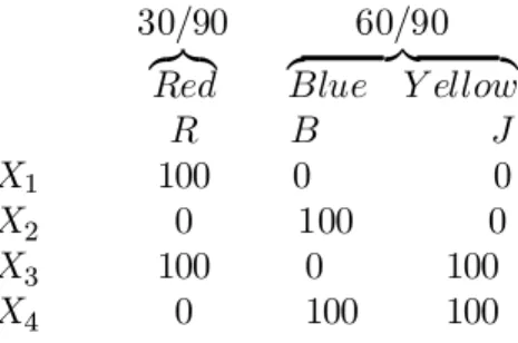
According to the importance of Ellsberg’s Paradox in order to construct ex-tensions of the classical models, we just recall it here, although it has already been made explicit in chapter 2 of this volume. Ellsberg proposes to subjects the following situation: an urn contains 90 balls, whose 30 are red (R) and whose 60 are blue (B) or yellow (Y), in unknown proportion. So the number of blue balls may be from 0 to 60 and the complement consists of yellow balls. One will draw (at random) one ball from the urn and one asks the subjects to choose between the two following decisions: bet on (R) (decision X1) or bet
on (B) (decision X2), then, independently, to choose between the following
decisions: bet on (R [ Y ) (decision X3) or bet on (B [ Y ) (decision X4).
2.1.1 Interpretation of Ellsberg’s paradox in the framework of Sav-age
Table 3.1 gives, for each decision the corresponding values of consequences (expressed in euros) of each decision according to the occurred event.
30=90 60=90
z}|{
Red zBlue Y ellow}| {
R B J
X1 100 0 0
X2 0 100 0
X3 100 0 100
X4 0 100 100
Typically a majority of subjects make the following choices : X1Â X2and
X4 Â X3, consequently, as it has been proved in the previous chapter, such
a behavior is incompatible with the Savage Sure-Thing Principle , one of the major axiom of the theory.
Moreover, as noticed by Machina and Schmeidler (1992), such subjects are not even probabilistically sophisticated : this means that they do not ascribe subjective probabilities pR; pB; pY to states of nature (i.e. elementary
events R; B; Y ) and then use …rst order stochastic dominance axiom2 - a widely
2Let us recall that, if X and Y are real random variables, the …rst order stochastic
dominance rule stipulates that if 8t 2 R; P fX ¸ tg ¸ P fY ¸ tg ; then X should be weakly preferred to Y , the preference becoming strict if P fX ¸ tg > P fY ¸ tg , for some t02 R.
accepted rule for partially ordered random variables. Otherwise, g1Â g2would
imply pR> pB and g4 Â g3 would imply pB+ pY > pR+ pY : a contradiction.
2.1.2 Interpretation of Ellsberg’s paradox in Anscomb and Au-mann framework
In the previous presentation of Ellsberg paradox, uncertainty is modelled through the set of the states of the world S0 = fR; B; Jg and bets are
in-terpreted as mappings X : S0! R:
We have seen, in chapter 2 of this volume, that Ellsberg’s paradox is robust when, as Schmeidler (1989), one considers Ellsberg’s experiment in the context of Anscombe & Aumann (1963) : actually it turns out that the independence axiom AA3 is violated.
Uncertainty now concerns the composition of the urn: the set S of states of nature is composed of 61 states : S = fs0; s1; :::; sk; :::; s60g;where a state
sk stands for a given composition of the urn : ”30 red balls, k blue balls and
60¡ k yellow balls ”.
Let us call Y the set of all lotteries on C = f0;100g, or equally of all probability distributions on C with …nite support. The uncertain prospect described by the act Xi in the Savage framework is now characterized in the
framework of Anscombe and Aumann, by the mapping gi from S to Y, gi:
S! Y in the following way:
To each state of nature sk of S, the consequence gi(sk) is the lottery :
(Xi(R); 30=90 ; Xi(B); k=90 ; Xi(J ); (60¡ k)=90 ); or equally the lottery
o¤ering Xi(R) with probability 3090, Xi(B) with probability90k, and Xi(J ) with
probability (60 ¡ k)=90 (see table 2.2 linked with the various acts in chapter 2 of this volume, paragraph 2.4.4).
If one assumes, as implicitly done by Schmeidler and Anscombe-Aumann that, under risk, the decison maker maximizes an expected utility (see Chapter 1 of this volume) with a von Neumann utility function u (which can be as-sumed without loss of generality such that u(0) = 0; u(100) = 1), one can also establish through a direct computation that, in the Anscombe-Aumann framework, the expected utility model under uncertainty cannot explain pref-erences described above : actually imagine that the decision-maker ascribes probabilities to the events sk, and that he behaves in accordance with the
Anscombe-Aumann expected utility model, i.e. prefers h to g if and only if Ppku(h(sk)) ¸ Ppku(g(sk)): Then, a simple computation shows that
g1 Â g2 would give 30 > Pkpk while g4 Â g3would give 30 < Pkpk; a
contradiction.
2.2 Schmeidler’s model in Anscombe-Aumann’s framework
In order to explain such ”paradoxes” and to separate perception of uncer-tainty from valuation of outcomes, Schmeidler (1989) has proposed a model
which relaxes the usual independence condition while o¤ering a ‡exible but simple formula. As was previously pointed out, Schmeidler (1982, 1989) has developed his model in the Anscombe-Aumann’s framework. Hence, in this section, the set S of sets of nature is …nite and the events are the elements of E = 2S. The set of consequences Y is the set of lotteries on a given set
of outcomes C (i.e. Y is the set of probability distributions on C with …nite support). The set of acts is the set of mappings F0 from S to Y also called
"horse lotteries". Let % be the preference relation of the decision-maker on the setF0.
2.2.1 Comonotonic independence
Let us recall that, in Anscombe-Aumann framework, the subjective expected utility model , SEU (see Chapter 2 of this volume), obtains mainly through the following axiom:
Axiom 1 Independence axiom (Anscombe and Aumann)
For all f; g; h inF0, and for all ® in ]0; 1[: f  g implies ®f + (1 ¡ ®)h Â
®g + (1¡ ®)h:
We have seen that a great majority of behaviors contradict such an axiom (Interpretation of Ellsberg’s paradox in Anscomb and Aumann). In order to weaken this axiom, Schmeidler introduced the de…nition of comonotonic acts and then the following weakened axiom:
Axiom 2 Axiom of comonotonic independence (Schmeidler)
For all acts f, g and h in F0 , pairwise comonotonic and for all ® in
]0; 1[: f g implies ®f + (1 ¡ ®)h  ®g + (1 ¡ ®)h:
Roughly speaking, comonotonic independence requires the direction of preferences to be retained, provided hedging e¤ects are not involved. This intuition which is crucial in Schmeidler’s model, will appear more transparent in Schmeidler’s representation theorem (1989).
By adding to this key axiom, some usual axioms as weak order and continu-ity, Schmeidler (1989) derives the characterization of his model where typical preferences observed in paragraph 3.2.1 become admissible.
2.2.2 Representation of preferences by a Choquet integral in Anscombe-Aumann’s framework
Schmeidler shows that the preference relation% on F0(the acts in
Anscombe-Aumann’s framework) satisfying the axioms previously described is represen-ted by a Choquet integral with respect to a unique capacity v. More precisely, For all f and g in F0 : f % g if and only if RChu(f (:))dv¸RChu(g(:))dv
where u is the von Neumann utility function on the set Y of lotteries on C.
Notice that capacity v is substituted to probability P in Anscombe-Aumann’s theorem.
The strategy of Schmeidler’s proof consists in …rst noting that axiom 2 entails axiom 1 on the set of constant actsFc
0, hence the existence of a vNM
utility function u on the set Y of lotteries, and therefore the ability of linking in a natural way any act f = (y1; A1; :::yn; An) =
i=nP i=1
yi1Ai;where yi 2 Y; with
the real random variable u(f) =i=nP
i=1
xi1Ai;where xi = u(yi); i = 1; ::n.
Then denoting by X0 the set of such variables, Schmeidler shows in a
second step that the preorder induced on X0, denoted%0 is representable by
a Choquet integral, equally, that there exists a capacity v on S such that: 8(X; Y ) 2 X2
0; X %0 Y () RChX dv¸RChY dv
2.3 Choquet expected utility (CEU) models in Savage’s
frame-work
By Choquet expected utility (CEU) models, we mean those non-additive mod-els directly connected with the Choquet integral which, following pioneer’s work of Schmeidler (1982, 1989) in the Anscombe-Aumann framework, have been derived in Savage framework as for example by Gilboa (1987) or Wak-ker(1990).
Savage framework seems more natural than Anscombe-Aumann one’s where consequences are lotteries but there the axiomatization becomes more soph-isticated.
Although Savage framework allows for more general consequence sets C, we will con…ne in this paragraph 2.3. to C = R, which permits a simple exposure of the main properties of CEU models.
So we consider a decision-maker making his choices inside the set X of acts consisting of all functions X : (S; E)! R, E-measurable and bounded where S is a set of states of nature and E a ¾-algebra of subsets of S. This decision-maker is in a situation of uncertainty, and% is a preference relation onX.
2.3.1 Simpli…ed version of Schmeidler’s model in Savage’s frame-work
In this framework, referred to as Savage’s framework, and which …ts the …rst and simple presentation of Ellsberg’s paradox, a simpli…ed translation of the comonotonic independence axiom of Schmeidler is as follows :
Axiom 3 Axiom of comonotonic independence (Chateauneuf, (1994)): LetX; Y; ; Z 2 V; X et Z comonotonic, Y and Z comonotonic,
where for C = R, the de…nition of comonotonic acts is the one of de…nition 2.
Axiom 3.3?? of comonotonic independence requires to maintain the dir-ection of preferences when adding the same act, as soon as no asymmetric reduction of uncertainty is involved through hedging e¤ects. On the contrary, in case of asymmetric reduction of uncertainty ( through hedging e¤ects), axiom 3.3?? allows for modifying the direction of preferences.
Example 3.1 below shows how such a behavior under uncertainty can be taken into account in a case where the acts give results depending of the realization of the event A or of the complementary event A._
Example 1 A A X 25000 15000 Y 12000 30000 Z 15000 25000 X + Z 40000 40000 Y + Z 27000 55000
Assume at the beginning indi¤erence between X and Y (X » Y ): Z is comonotonic with Y but not with X, Z may be used as a hedge against X but not against Y , and consequently an uncertain averse decision-maker may express after addition of the variable Z, the following strict preference : X + ZÂ Y + Z:
Under the key comonotonic independence axiom and other classical axioms as weak order and continuity, it is then possible to deduce from these axioms a simpli…ed version of Schmeidler’s model where preferences can be represented by a Choquet integral with respect to a capacity v, i.e.:
For all X; Y 2 X; X % Y if and only if RChXdv ¸
R
ChY dv (see
Chat-eauneuf(1994)).
Note that this model is simpli…ed in the sense that utility of outcomes is linear, a consequence of the independence axiom of Chateauneuf (1994).
Such a result is deduced from the fundamental theorem of Schmeidler (1986), which characterizes the Choquet integral (1953)), and appears as a crucial tool for Schmeidler’s model and more generally for Choquet expected utility(CEU) models .
2.3.2 Choquet expected utility model in Savage’s framework When utility of results is no longer necessarily linear, one gets the following classical de…nition of the Choquet expected utility model:
De…nition 5 A decision-maker satis…es the Choquet expected utility (CEU) model if the decision-maker’s preferences on the set of actsV can be represented
with the help of a utility function under certainty u: R ! R, non-decreasing and de…ned up to an increasing a¢ne transformation and with the help of a personal evaluation of the likelihood of events through a capacity v. Preferences representation is given by I(u(X)) =RChu(X)dv, the Choquet integral of u(X) with respect to capacity v, de…ned for X 2 X by
Z Ch u(X )dv = Z 0 ¡1 [v(u(X) > t)¡ 1] dt + Z 1 0 [v(u(X) > t)] dt (3) Note that this CEU model generalizes equation (1) with a function u which is not necessarily linear.
For a simple step act X = (x1; A1; :::; xn; An) = i=nP i=1
xi1Aiwhere xi 2 R;
Ai 2 E; (Ai) partition of S; one obtains :
R
Chu(X)dv =
u(x1) + (u(x2)¡ u(x1))v [X¸ x2] + ::: + (u(xn)¡ u(xn¡1))v [X¸ xn] :
Remark 1 One can interpret the behavior of a decision-maker using this modelRChu(X)dv as follows: The decision-maker values X by …rst evaluating the utility of the minimum result x1 he gets with certainty, and then adding
the additional increases of utility u(xi+1)¡ u(xi); 1 · i · n ¡ 1; weighted by
his personal belief v [X ¸ xi+1] of their occurence.
Example of computation of such a Choquet integral Let S = fs1; s2; s3g:
Let v be a capacity on S as below and X an act such that the values of u(X ) are given in the following table:
Á s1 s2 s3 s1[ s2 s1[ s3 s2[ s3 S
v 0 1=3 0 0 1=3 1=3 2=3 1
u(X) a b c
The evaluation of the Choquet integral I =RChu(X)dv depends of the ranking of a; b; c : ² if a < b < c,RChu(X)dv = a + (b¡ a)v(fs2; s3g) + (c ¡ b)v(fs3g) = 1=3a + 2=3b ² if c < a < b,RChu(X)dv = 2=3c + 1=3a ² if b < c < a,RChu(X)dv = 2=3b + 1=3a ² ::::
A classical integral, with an additive measure, would naturally take the same value whatever be the ranking of consequences.
2.3.3 The comonotonic sure thing principle
The main feature of the CEU model is to allow taking into account possible hedging e¤ects. For this purpose, the crucial axiom in the axiomatization of CEU, is the comonotonic sure thing principle (see for instance, Gilboa (1987), Chew and Wakker (1996)), a weakening of Savage’s sure thing principle, which can be stated in the following way :
Axiom 4 The comonotonic sure thing principle Let X = Pn i=1 xi1Ai et Y = n P i=1
yi1Ai, where fAig is a partition of S and
x1 · ::: · xi · ::: · xn ; y1· ::: · yi · ::: · yn are such that xi0 = yi0 pour
some 1 · i0· n. Then X % Y implies X0% Y0 for the acts X0et Y0obtained
from acts X and Y by merely replacing the iemeµ
0 common result by any other
common result which preserves the ranking i0for both acts X and Y .
This axiom expresses that, as long as acts remain comonotonic (i.e., no hedging e¤ect happens), there is no reason to change the direction of prefer-ences when a common outcome is modi…ed.
Note, however, that even jointly with standard axioms of weak order, con-tinuity and monotonicity, the comonotonic sure-thing principle fails to fully characterize CEU.
For instance, Wakker (1989) completes the axiomatization of the CEU model by strengthening axiom 3.4 to a ”comonotonic trade-o¤ consistency” one.
We now turn to the ability of Schmeidler’s model to handle uncertainty aversion (and symmetrically uncertainty appeal).
2.4 Uncertainty aversion
In his seminal papers, Schmeidler (1982, 1989) has shown the great ability of his model to capture the concept of uncertainty aversion. He de…ned un-certainty aversion through convexity of preferences i.e. : 8f;g 2 F0;8® 2
[0; 1] ; f » g ) ®f + (1 ¡ ®)g % f , interpreting this axiom as ”smoothing” or averaging potential outcomes makes the DM better o¤. This de…nition re-vealed as particularly meaningful since as proved by Schmeidler (1986, 1989), uncertainty aversion is equivalent to the capacity v being convex and since furthermore one has :
Proposition 2 Schmeidler(1986)
Let I :X ! R be a Choquet integral with respect to a capacity v, i.e.8X 2 X; I(X) =RChXdv, then the two following conditions are equivalent:
(i) v is convex ;
(ii) Core(v) 6= Á where core(v) = ½
simply additive probabilitiesPonE t.q. P(A) ¸ v(A); 8A 2 E
¾ and for all X inX : RChXdv = Min©RXdP; P 2 core(v)ª.
This proposition o¤ers an attractive interpretation of uncertainty aversion in terms of pessimism : in Schmeidler’s model, an uncertainty averse decision-maker, behaves in the following way: he considers for every act, among all probability distributions P in core of v, the one giving the minimum expected utility EPu(f ) of this act, and then chooses the act which maximizes this
minimum :
i.e. 8f;g 2 F0; f % g i¤ Min P2core(v) R S u(f )dP ¸ Min P2core(v) R S u(g)dP:
Such an interpretation would remain true for the CEU model (i.e. in Sav-age’s framework) since for such a model, convexity of preferences is equivalent to v convex and u concave (see Chateauneuf and Tallon (2002)).
Moreover, in the simple case of the CEU model with constant marginal utility (u(x) = x; 8x 2 R); one can give directly an interpretation in terms of hedging e¤ects, since there, convexity of preferences is equivalent to the following uncertainty aversion axiom (Chateauneuf (1994)):
Axiom 5 Uncertainty aversion3
For X; Y; Z2 X; Y et Z comonotonic, then X » Y ) X + Z % Y + Z Notice that this uncertainty aversion axiom implies the comonotonic inde-pendence axiom and therefore characterizes the simpli…ed Schmeidler’s model, where, moreover, v is convex.
This axiom allows for taking into account hedging e¤ects : since Z is not a hedge against Y but may be a hedge against X, hence X + Z may display a reduction of uncertainty with respect to Y + Z, and therefore X + Z may be preferred to Y + Z by an uncertainty averse DM.
Such an interpretation …ts particularly well for interpreting behaviors in Ellsberg’s example : let us describe uncertainty in Ellsberg’s example -in ac-cordance with paragraph 3.2.1- by : S = fR;B; Y g ;E = 2S: Let P be the
set of all probability distributions on (S; 2S) compatible with the information
(i.e. P =©probability distributions on (S; 2S) such that P (R) = 1=3ª and let
v de…ned by v(A) = Inf
P
P(A);8A 2 E ; one obtains table 3.3.??
Á R B Y R[ B R [ Y B[ Y S
v 0 1/3 0 0 1/3 1/3 2/3 1
It is straightforward to show that v is a convex capacity4 and that P =
core(v).
3a completer 4
Let us compute I(X) =RChX dv for all considered acts : I(X1) = 1=3£ 100 > I(X2) = 0£ 100; thus X1Â X2
I(X4) = 2=3£ 100 > I(X3) = 1=3£ 100; thus X4Â X3
Consequently one can explain the behaviors in Ellsberg’s paradox by uncer-tainty aversion.
2.5 The multi-prior model
We now consider the model “max-min” of Gilboa and Schmeidler (1989). In this model, the agents have a set of a priori probability laws (and not a single one as in the Bayesian paradigm ) and use the maximin criterion for evaluating decisions through this set of initial beliefs (multiple prior).
2.5.1 The axiomatic of the model
Gilboa and Schmeidler (1989) consider an Anscombe-Aumann framework (1963), where the set of consequences is a set Y of laws with …nite support over a set C. This axiomatic is very simple and leans mainly on the two following axioms. The …rst one is axiom 3.6?? of certainty independence:
Axiom 6 For all f; g of F0and h constant decision of F0, for all ® 2]0;1[
f  g =) ®f + (1 ¡ ®)h  ®g + (1 ¡ ®)h
This axiom is weaker than the usual independence axiom, since it applies only when adding a "common consequence" which is constant. This axiom is implied by the comonotonic independence axiom (axiom 3). The second axiom is the one of uncertainty aversion previously de…ned in Schmeidler’s model(1989) :
Axiom 7 For all f; g in F0 and ® 2]0;1[
f s g =) ®f + (1 ¡ ®)g % f
Proposition 3 (Gilboa and Schmeidler (1989)) Under the axiom of weak or-der, an axiom of monotony, an axiom of continuity and the axioms 6 and 7, there exists a set of probability measures P, closed and convex, and a utility function u of von Neumann: Y ! R such that:
f % g () min P2P Z u(f)dP ¸ min P2P Z u(g)dP
THe function u is unique up to a positive a¢ne transformation, while the set P is unique if closed in the weak-star topology.
The interpretation of this representation is fairly simple. The decision-maker behaves as if he had a set of a prior beliefs (instead of a unique one as in the expected utility model). In order to evaluate an act, he computes the expected utility of this act with respect to all probability distributions that he considers in P, and then takes the minimum. This last operation …ts to a pessimism attitude or uncertainty aversion. Note that by construction, this model can only take into account pessimistic behaviors and not “optimistic” behaviors or mixed behaviors.
2.5.2 Comparing multi-prior model with Choquet utility model The multi-prior model is closely linked with the Choquet utility model. With this model, it is possible to interpret the Choquet capacity in terms of beliefs. Actually, from proposition 2 :
v is convex () ½
core(v)6= ; and R
Chu(X)dv = minP2core(v)R u(X)dP for all X2 X
When the decision-maker’s capacity is convex, this decision maker behaves as in a multi-prior model whose set of probability measures is given by the core of the capacity. The multi-prior model allows to give an “objective” foundation to the (subjective) capacity of the Choquet utility model; capacity which then represents the lower envelope of the family of probability measures of the capacity of the multi-prior model. Nevertheless, one should notice that every closed and convex family of probability measures is not necessarily the core of a convex capacity and therefore that the multi-prior model is not a particular case of the Choquet utility case with a convex capacity. Moreover the behaviors described by a Choquet integral with respect to a non-convex capacity cannot be described by the multi-prior model.
Remark 2 The behavior of a decision-maker of the multi-prior type may be considered as excessively pessimistic. In fact, in the next section we present the models of Ja¤ray (1989a, 1989b) and Ja¤ray-Philippe (1997) which model less extreme behaviors.
2.5.3 CEU model and lower and upper envelopes of a family of probability distributions
Ja¤ray (1989a, 1989b) and Ja¤ray and Philippe (1997) have proven that, under some conditions, it was possible to write a Choquet integral with respect to any capacity v as a linear combination ?? of two terms :respectively the minimum and the maximum of expected utilities with respect to a family of probability distributions, the weight between the two representing an index of pessimism.
As we showed previously, in the Ellsberg experiment, the uncertainty can be summarized by the lower envelope v(:) = Inf
P2P
P (:), and in this case, this capacity v is convex, allowing thus simpler formula, as we showed in propos-ition 2. ; indeed, if v is a convex capacity on (S; E), then 8X 2 X, min ©R
XdP; P 2 core(v)ª=RChXdv:
Such situations of uncertainty, summarized by a lower envelope (i.e. a convex capacity) have been de…ned by Ja¤ray (1989a, 1989b) as being "regular uncertainty"
De…nition 6 We are in a situation of regular uncertainty when the situation of uncertainty, de…ned by a family of probability distributions P on (S; E) is completely characterized by its lower envelope c where c(A) = Inf
P2PP(A) and c
is convex, meaning that P ={ P on (S; 2S); P ¸ cg. We will denote by C the
upper envelope of P : C = Sup
P2PP (:) and C(A) = 1¡ c( _
A); 8A 2 E):
This "regular uncertainty" can be encountered in natural situations as shown by Dempster (1967). Let us assume (as in Dempster) that (-; 2-; ¼) is a
…nite probability space and that ¡ is a correspondence from - to E¤=E ¡fÁg,
where E = 2S and S is a …nite state space. Let us interpret ¡ as informing us
that if $ 2 - occurs, then the true state s belongs to ¡($) (such a state space (-; 2-; ¼) is called a message space) ; one can then states that each event A2 E
occurs with a probability at least equal to v(A) where v(A) = P
B½A
m(B), and
m(B) = P
f$2-;¡($)=Bg
¡(f$g); it can be shown that v is a belief function (i.e. a particular case of a convex capacity (see for instance Shafer (1976) and chapter 3 in …rst volume??).
Now, in such situations of regular uncertainty ; it can be the case that a CEU decision maker don’t have necessarily uncertainty aversion ( i.e. does not have necessarily a subjective assessment of events represented by a capacity v = c, but by a subjective assessment of events represented by a capacity v = ®c + (1¡ ®)C with ® 2 [0; 1] ; c being convex.
Such a behavior where the value of ® can be interpreted as the pessimism index due to Hurwicz, has been studied and axiomatized by Ja¤ray and Phil-ippe (1997) who have shown that this behavior was compatible both with the CEU model and with the Ja¤ray (1989a,1989b).
3 Decision under risk
From now, we assume that there is an "objective" probability distribution P on (S; E) and that the decision maker knows it ; we say then that the decision maker is facing a problem of decision under risk.
Moreover, to make the exposition simpler, we suppose that the probability distribution P is ¾¡additive and non-atomic (i.e. 8A 2 E; such that P (A) > 0; 8® 2 (0; 1] ; 9B 2 E; B ½ A , such that P(B) = ®P(A)) ; thanks to these assumptions, the set X of acts generate any real bounded random variable.
Any element X of X is then a random variable whose probability distri-bution is PX. Let us denote FX the cumulative distribution function of X
(8x 2 R; FX(x) = Pfs 2 S=X(s) · xg = PSfX · xg), E (X) its expected
value and L the set of all probability distributions of elements of X.
Since every X of X induces a probability distribution L(X) on R, the preference relation % on X also induces a preference relation on L that (by misuse of notation) we also denote by%, under the following condition H0:
Condition H0 (N eutrality): Two random variables with the same
probab-ility distribution are always indi¤erent.
Hence, under this condition, any axiomatization on (X, %) can be replaced by an axiomatization on (L, %).
Remark 3 Any discrete act X ofX can be written : X = (x1; A1; : : : ; xk; Ak;
: : : ; xn; An), where (Ai) (i = 1; :::; n) is a partition of S and xithe consequence
of X on each Ai:Under risk, the probability distribution of this random variable
will be denoted : L(X) = (x1; p1; : : : ; xk; pk; : : : ; xn; pn) with x1 · x2 ·
¢ ¢ ¢ · xn, pi= P (Ai)¸ 0, and Ppi = 1.
In the following, it can be useful to use also the following notation : L(X) = (x1; 1¡ q1; x2; q1¡ q2; : : : ; xn¡1; qn¡2¡ qn¡1; xn; qn¡1) (4)
where, for i = 1; :::n ¡ 1, qi= j=nP j=i+1
pj.
In this section, we identify any consequence c with its Dirac probability distribution ±fcg.
3.1 EU model and Allais paradox
We have study in detail, in chapter 1 of this volume, the classical model of decision under risk : the Expected Utility (EU) model . As early as 1953, Allais has built a couple of alternatives for which a majority of subjects, confronted with that choices, choose in contradiction with the independence axiom and thus in violation with the EU model (see chapter 1, section 1.4.1.).
Since this experiment, known as Allais "paradox", has been a cornerstone to question the EU model, let us …rst recall, in this chapter, the original Allais paradox (Allais (1953)).
Subjects were asked to choose between the following lotteries (say in thou-sand euros):
L1 : win 1M with certainty or L2 : win 1M with probability 0.89, 5M
and then independently, to choose between the following lotteries: L0
1: win 1M with probability 0.11 and 0 with probability 0.89 or
L02: win 5M with probability 0.10 and 0 with probability 0.90.
Most subjects choose L1 over L2, and L0
2 over L01. These simultaneous
choices violate the independence axiom. Indeed, de…ning P as the lottery yield-ing 1 M with probability 1 and Q as the lottery yieldyield-ing 0 with probability 1=11 and 5 M with probability 10=11, one can check that:
L1 = 0; 11P + 0; 89±1
L2 = 0; 11Q + 0; 89±1
L01 = 0; 11P + 0; 89±0
L02 = 0; 11Q + 0; 89±0
where ±0 is the lottery “win 0 with probability 1” and ±1is the lottery “win
1 M with probability 1 ”. The observed choices are thus in contradiction with the independence axiom5.
This experiment has been ran many times, on various populations of sub-jects with similar results: about 66% of the choices are in contradiction with the independence axiom.
Not only observed behaviors are in contradiction with EU theory, but also the EU model raised a theoretical di¢culty, namely, the interpretation of the function u (called von Neumann’s utility) characterizing the DM’s behavior : as pointed out by Allais himself, the function u has, in fact a double role of expressing the DM’s attitude with respect to risk (concavity of u implying risk aversion) and the DM’s valuation of di¤erences of preferences under certainty (concavity of u implying then diminishing marginal utility of wealth). These evidences have led researchers to built more ‡exible models. The RDU model that we will present in the next section, not only will disentangle attitude towards risk and satisfaction of outcomes, but also will be compatible with observed behaviors in Allais experiment.
3.2 The Rank Dependent Expected Utility model
3.2.1 De…nition of the Rank Dependent Expected Utility model The Rank Dependent Expected Utility (RDU) model is due to Quiggin (1982) under the denomination of "Anticipated Utility". Variants of this model are due to Yaari (1987), Segal (1987, 1993) and Allais (1988). More general axio-matizations can be found in Wakker (1994), Chateauneuf (1999).
De…nition 7 A DM behaves in accordance with the rank-dependent expected utility (RDU) model if the DM’s preferences on (L,º) are characterized by two
5since under independence axiom:
functions u and f: a continuous, increasing, cardinal6utility function u : R !
R (that plays the role of utility on certainty) and an increasing probability -transformation function f : [0; 1] ! [0; 1] that satis…es f(0) = 0; f(1) = 1. Such a DM prefers the random variable X to the random variable Y if and only if V (X) ¸ V (Y ), where the functional V is given by :
V (Z) = Vu;f(Z) = Z 0 ¡1 [f (P (u(Z) > t))¡ 1] dt + Z 1 0 f (P (u(Z) > t))dt : (5) ² If the transformation function f is the identity function f(p) ´ p, then V (Z) = Vu;I(Z) is the expected utility E[u(Z)] of the random variable
Z.
² If the utility u is the identity function u(x) ´ x, then V (Z) = VI;f(Z)
is theYaari functional (see Yaari (1987)). In fact, Yaari axiomatized independently his model7 .
² If both transformation and utility are identity functions, then V (Z) = VI;I(Z) is simply the expected value E[Z] of the random variable Z.
When Z is discrete, V (Z) can be written as
V (Z) = u(x1)+f (q1)[u(x2)¡u(x1)]+ ::+f (q2)[u(x3)¡u(x2)]+¢ ¢ ¢+f(qn¡1)[u(xn)¡u(xn¡1]
(6) We can then interpret the evaluation of a RDU decision maker: he evaluate …rst, for sure, the utility of the worst outcome u(x1) and then, weights the
additional possible increases of utility u(xi)¡ u(xi¡1) by his personal
trans-formation f(qi) of the probability vi of having at least xi.
According to this interpretation, if the decision maker behaves in such a way that f(p) · p; it means that he underestimates all the additional utilities of gains. In this sense, we will call him pessimistic under risk. In the same way, ure‡ecting now his satisfaction for wealth, concavity of u reveals diminishing marginal utility.
Remark 4 Let us notice that various attempts to generalize EU model by a functional likewise:
(x1; p1; : : : ; xk; pk; : : : ; xn; pn)7¡! Pf(pi)u(xi) with f : [0; 1] ¡! [0; 1]
and f(0) = 0, f(1) = 1; failed because the only functionals compatible with the …rst order stochastic dominance is obtained for f(p) = p, meaning that this functional reduce to EU.
6
u is cardinal if it is de…ned up to an a¢ne increasing transformation.
7Yaari model is called "Dual Theory". This model is as parcimonious as EU model since
it used only one function f ; however, this model allows to distinguish strong risk aversion from weak risk aversion, which is not possible in EU model.
Allais "Paradox" is compatible with RDU model As an exercise, we can evaluate in a RDU model the di¤erent lotteries of Allais example. setting (w.l.o.g.) u(0) = 0;we have
V (L1) = u(1) ; V (L2) = u(1)(f (0:99)¡ f(:0:10)) + u(5)f(0:10) ;
V(L0
1) = u(1)f (0:11) and V (L02) = u(5)f (0:10):
L1Â L2implies u(5)f(0:10) < u(1)[1¡f(0:99)+f(0:10)] ; L02Â L01implies
u(5)f (0:10) > u(1)f (0:11) ;so that the simultaneous choices L1Â L2and L02Â
L01are explainable by RDU theory for any f satisfying :1¡f(099) > f(0:11)¡ f (0:10); revealing that the same probability di¤erence 0:01 is considered as more important in the neighborhood of certainty.
3.2.2 Key axiom of RDU’s axiomatization : comonotonic sure-thing principle
The key axiom of the RDU model is the following :
Axiom 8 Comonotonic Sure-Thing Principle under risk8 :
Let P, and Q be two lotteries of L. P = (x1; p1; : : : ; xk; pk; : : : ; xn; pn) and
Q = (y1; p1; : : : ; yk; pk; : : : ; yn; pn) be such that xk0 = yk0 ; then P º Q implies
P0º Q0 for lotteries obtained from lotteries P and Q by merely replacing the kth
0 common outcome xi0, by a common outcome x0k0 again in k
th
0 rank both
in P0and Q0:
This axiom from Chateauneuf (1999), is very similar to Green and Ju-lien’s ordinal independence axiom (1988), to Segal’s irrelevance axiom (1987), and comonotonic independence in Chew and Wakker (1996)( see also Chew-Epstein (1989), Quiggin (1989), Wakker, (1994) ; it is clearly much weaker than Savage’s sure-thing principle that requires no restriction on x’i0:
Remark 5 In the statement of this axiom, the common modi…cation of the two lotteries do not change the order of the common outcomes in their respect-ive distributions. The corresponding random variables canonically associated to the distributions ( X and Y taking respectively values xk and yk on sets
Ek with probability pk(k = 1; ::n) stay comonotonic.
To capture the real meaning of this axiom, let us come back to Allais’ experiment where subjects have to chose …rst between L1 and L2;then
in-dependently, between L0
1 and L02 where the 4 lotteries are indicated in the
following table:
8The justi…cation of the denomination of this axiom results from a natural interpretation
Pr Probabilities 0; 01 0; 89 0; 1 L1 1 M 1 M 1 M Lotteries L2 0 1 M 5 M L01 1 M 0 1 M L02 0 0 5 M
The common modi…cation from L1 to L01 and from L2to L02does not
pre-serve the rank of the common outcome in the both modi…ed lotteries : more precisely, the common value 1M (with proba0.89) in L1and L2corresponds to
an intermediate value whereas the common value 0M (with the same probab-ility) corresponds to the smallest value. Thus, the two choices L1and L02do
not contradict the previous Comonotonic Sure-Thing Principle.
A complete characterization of RDU model can be, for instance, obtained with the help of noncontradictory comonotonic trade-o¤s (see Wakker (1994)), or else with a comonotonic mixture independence axiom, an adaptation of mix-ture independence, which underlines the role played not only by comonotony, but also by the extreme outcomes (see Chateauneuf, 1998).
This attractive axiom is a central necessary axiom in the characterization of RDU, but, as in the case of CEU, even jointly with the standard axioms of weak order, continuity, monotony, this axiom fails to fully characterize RDU. A complete characterization of RDU model can be, for instance, obtained with the help of noncontradictory comonotonic trade-o¤s (see Wakker (1994)), or else with a comonotonic mixture independence axiom, an adaptation of mix-ture independence, which underlines the role played not only by comonotony, but also by the extrema outcomes (see Chateauneuf, 1998).
More precisely, to characterize RDU model, Chateauneuf adds to the usual axioms of weak order, monotony, continuity and the Comonotonic Sure-Thing Principle under risk, the following axiom :
Axiom 9 Comonotonic Mixture Independence Axiom
For every p in [0; 1], (1)P1= (1¡ p)±x1 + p±a » Q1= (1¡ p)±y1 + p±band
(2)P2= (1¡ p)±x1 + p±c » Q2= (1¡ p)±y1 + p±d imply
(3)®P1+ (1¡ ®)P2» ®Q1+ (1¡ ®)Q2;for every ® in [0; 1] ;
For every p in [0; 1], (4)R1= (1¡ p)±a+ p±z1 » S1= (1¡ p)±b+ p±t1 and
(5)R2= (1¡ p)±c+ p±z1 » S2= (1¡ p)±d+ p±t1 imply
(6)®R1+ (1¡ ®)R2» ®S1+ (1¡ ®)S2;for every ® in [0; 1]:
This axiom underlines the role played not only by comonomonicity but also by the security factors x1and y1in (1) and (2)and potential factors ( z1
and t1 in (4) and (5) (see Ja¤ray’s model (1988) and Cohen’s model (1992)
3.3 From CEU model to RDU model using …rst order stochastic
dominance (Wakker)
Let us …rst show that the RDU representation can be viewed as a Choquet integral .
3.3.1 RDU representation is a Choquet integral
In the RDU model, the function f from [0; 1] to [0; 1] is increasing and satis…es f(0) = 0 and f(1) = 1. The corresponding "transformed" probability f oP is thus a capacity and the RDU functional is a Choquet integral with respect to this capacity v = foP . More precisely,
V (Z) =RChu(Z)d(foP) =¡R¡11 u(x)df (P(Z > x)) =¡R¡11 u(x)df (1¡ F (x))
Remark 6 Let us notice by now, that if f is a convex function, then v = foP is a convex capacity (see e.g. Chateauneuf, (1991) or Denneberg, (1994)). Moreover, if f is below the diagonal (i.e. satis…es f(p) · p; 8p 2 [0;1]), then it can be easily seen that core(v) 6= Á:
3.3.2 From CEU to RDU
It has been recognized by several authors including Wakker (1990), Chateau-neuf (1991), that RDU model under risk can be derived from CEU model under uncertainty by merely postulating the respect of …rst order stochastic dominance. We will use this approach, …rst to get Yaari’s model from the sim-pli…ed version of Schmeidler’s model (section 2.2??), then to get RDU model from Choquet Expected Utility model.
Being under risk, we suppose that the objective probability P is compatible with the preference relation on (V,º). More precisely, we suppose :
Axiom 10 First order stochastic dominance :(Pour Alain A revoir) [A; B2 A; P(A) ¸ P(B)] ) A º B:
Let us notice that this axiom is actually weaker than the …rst order stochastic dominance axiom but proves to be equivalent in this framework. This axiom implies also the neutrality axiom stated at the beginning of the section. From simpli…ed Schmeidler’s model to Yaari’s model Let us suppose that the preference relation on (V,º) satis…es, moreover the usual axioms of non-trivial weak-order, continuity, monotonicity, the comonotonic independ-ence axiom 2??,. The preferindepend-ence relation is then represented by a Choquet integral with respect to a capacity v such that A º B implies v(A) ¸ v(B): The axioms imply then that P(A) ¸ P(B) imply v(A) ¸ v(B):
This gives us an intuition of the result : There exists a unique transformed function f : increasing function f : [0; 1] ! [0; 1] satisfying f(0) = 0;f(1) = 1) such that v = foP .
It can then be readily seen that the simpli…ed Schmeidler’s model reduces to Yaari’s model under the assumption of …rst order stochastic dominance (Wakker, 1990, Chateauneuf, 1994).
From general CEU model to RDU model Let us suppose that the preference relation on (V,º) satis…es all the axioms to get general CEU model characterized by v and u (see de…nition ??), then, A º B implies v(A) ¸ v(B): If moreover, the objective measure P on S satis…es …rst order stochastic dominance, again, since P(A) ¸ P (B) imply v(A) ¸ v(B); there exists then a unique transformation function f such that v = foP. We get the following result due to Wakker (1990) :
Let the preference relation on (V,º) satis…es all the axioms to get gen-eral CEU, and let P be a probability distribution on S satisfying …rst order stochastic dominance, then the preference relation on (V,º) can be represented by the RDU model.
3.4 Di¤erent notions of Risk Aversion and their
characteriza-tion in the RDU model
In the chapter 1 (decision under risk : the classical model), we already de…ned two notions of Risk Aversion (RA) : strong RA and weak RA. In the EU model, both notions have the same characterization: concavity of u . Let us recall these two notions here, before de…ning other ones.
The most natural way to de…ne risk aversion is the following :
De…nition 8 a DM is weakly risk averse if he always prefers to any random variable X the certainty of its expected value E(X) ( weakly risk-seeking if he always prefers any random variable X the certainty to its expected value E(X),risk-neutral if he is always indi¤erent between X and E(X)).
An other possible way to de…ne some type of risk aversion is to de…ne it as aversion to some type of (mean preserving) increase in risk. All kinds of stochastic orders can then generate as many di¤erent kinds of risk aversion.
There exists, then, many di¤erent de…nitions of risk aversion but their di¤erent meanings have been hidden by the fact that, under expected utility theory, all are equivalent : they all reduce to the concavity of the utility function(see chapter 1, section 4.3.).
Let us give some usual de…nitions of (mean preserving) increase in risk and their corresponding de…nitions of risk aversion:
3.4.1 Strong risk aversion
Y is a general mean preserving increase in risk (MPIR) of X ifR¡1t FY(x)dx¸
Rt
¡1FX(x)dx for all t 2 R and
R+1
¡1 FY(x)dx =
R+1
¡1 FX(x)dx. This usual
concept of (mean preserving) increasing risk is classically used in economics, since Rothschild and Stiglitz (1970) and we de…ne the corresponding notion of strong risk aversion :
De…nition 9 A DM is then strongly risk averse if he is averse to any general (Mean Preserving) increase in risk, i.e. for any X and Y inV such that Y is a MPIR of X, he prefers X to Y (strongly risk seeking if he prefers Y to X , risk neutral if he is indi¤erent).
3.4.2 Monotone risk aversion
Quiggin (1992) brought to light that strong risk aversion may be a too strong concept, and introduced a new notion, monotone (mean-preserving) increase in risk, de…ned in terms of comonotonic random variables instead of a general mean-preserving increasing risk :
Y is a (mean preserving) monotone increase in risk (MPMIR) of X if and only if9 Y =
d X + Z, where Z is such that E(Z) = 0 and X and Z are
comonotonic.
Before giving an important property of this notion, let us recall that F¡1(p) = inffz 2 RjF(z) ¸ pg; and then we can interpret F¡1(p) as the
highest gain among the least favorable p% of the outcomes.
Property : Lansberger and Meilijson (1994b) have proved that for two random variables with equal mean this notion is equivalent to the statistical notion of "dispersion" introduced by Bickel and Lehmann (1976, 1979): Y is more dispersed than X if
FY¡1(q)¡ FY¡1(p)¸ FX¡1(q)¡ FX¡1(p); where F¡1is de…ned from (0; 1] into R by F¡1(p) = inffz 2 RjF(z) ¸ pg, for all 0 < p < q < 1.
Thus, if Y is MPMIR of X, all the interquantile intervals are shorter for X than for Y . Let us then de…ne the corresponding notion of Monotone Risk Aversion.
De…nition 10 A DM is monotone risk averse if he is averse to any monotone increase in risk i.e. for every pair (X,Y) where Y is MIR of X, he always prefers X to Y (monotone risk-seeking if he always prefers Y to X, risk-neutral if he is always indi¤erent between X and Y:
This notion of monotone risk aversion10 is particularly …tted to RDU
the-ory where comonotony plays a fundamental part at the axiomatic level.
9
=
d means equality of probability distributions.
3.4.3 Left monotone risk aversion
The order induced by monotone increasing risk is a very partial order since it can order very few pairs of random variables. The following notion compares more pairs and this notion of increasing risk is asymmetric in the sense that it treats di¤erently downside and upside risks. This notion will prove to be particularly …tted with deductible insurance (see Vergnaud, 1997).
The following de…nition is due to Jewitt11(1989) under the name of
Location-independent Risk (see also Lansberger and Meilijson (1994a). The motivation of Jewitt was to …nd a notion of increase in risk that models coherent behavior in a context of partial insurance12.
Y is said to be a left monotone mean preserving increase in risk (LIR) of X if RFY¡1(p)
¡1 FY(x)dx¸
RFX¡1(p)
¡1 FX(x)dx for all p2 (0; 1).
Again, we de…ne the corresponding notion of left monotone risk aversion : De…nition 11 A DM is left monotone risk averse (respectively, left mono-tone risk seeking) if he is averse to any left monomono-tone increase in risk, i.e. for any X and Y in V such that Y is a left monotone MPIR of X, the DM prefers X to Y (respectively, Y to X).
Remark 7 It can be readily seen that Strong risk aversion )Left motone risk aversion) Monotone risk aversion ) Weak risk aversion. The reverse implications are not true, in general. However, in the EU model, all these notions are equivallent and are reduced to the concavity of u.
3.4.4 Characterization of di¤erent notions of risk aversion in the RDU model
Contrary to EU model, in the RDU model, each of the di¤erent notions of aversion to risk has a speci…c characterization13. Gathering several results in
di¤erent papers, we get the following results.
Let a RDU decision maker be characterized by two di¤erentiable functions uand f :
1. A RDU Decision Maker is then strongly risk averse (respectively strongly risk-seeking) if and only if the utility function u is concave and the transformation function f is convex (respectively uconvex and f concave) (see Chew, Karni and Safra, 1987).14
1 1In Jewitt, the notion is given for X and Y with possibly di¤erent means. 1 2See also Lansberger and Meilijson (1994a) on this subject.
1 3Machina (1982a, 1982b) was the …rst to notice that the equivalence between di¤erent
notions of risk aversion in the EU model does not carry over to generalized models.
2. A RDU Decision Maker is left monotone risk averse if and only if his transformation function f is star-shaped at 1 from above15and his utility
function u is concave (see Chateauneuf, Cohen and Meilijson, 2004). 3. A RDU Decision Maker is left monotone risk-seeking if and only if the
transformation function f is star-shaped at 1 from below 16 and the
util-ity function u is convex (see Chateauneuf, Cohen and Meilijson, 2004). 4. The characterization of monotone risk aversion is based on two following
indices : Pf = inf 0<v<1[
1¡f(v)
f (v) =1¡vv ], called index of pessimism, which is
¸ 1 as soon as f(p) · p, and Gu = sup y·xu
0(x)=u0(y), called index of
non-concavity17 (or greediness), which always satis…es Gu ¸ 1, and where
the value 1 corresponds exclusively to concavity.
A RDU Decision Maker with probability transformation function f and di¤erentiable utility u is monotone risk averse if and only if his index of pessimism is greater than his index of non-concavity, i.e. Pf ¸ Gu
(see Chateauneuf, Cohen and Meilijson, 2005). The most signi…cant feature of this result is that a DM does not need to have a concave utility function u to be monotone risk averse.
5. The characterization of monotone risk-seeking is based on two following indices : Of = inf0<v<1[1¡f(v)f(v) =1¡vv ] called index of optimism, which is
¸ 1 as soon as f(p) > p, and Tu = supx<y u
0(x)
u0(y), called index of
non-convexity , which always satis…es Tu ¸ 1 and the value 1 corresponds
exclusively to convexity.
A RDEU DM with probability perception function f and utility function u is monotone risk-seeking if and only if the DM’s index of optimism exceeds the DM’s index of non-convexity: Of ¸ Tu.
6. For a weak risk averse RDU decision maker, there is no known char-acterization but su¢cient conditions, not implying concavity of u (see Chateauneuf and Cohen, 1994).
The interesting point of all these results is that RDU models not only allow to separate transformation of probability from valuation of outcomes but moreover explain much diversi…ed behaviors as, for instance, to be weakly risk-seeking with a diminishing marginal utility of wealth or to dislike risk (to
1 5A transformation function f: [0; 1] to[0; 1] is star-shaped at 1 from above if for any x of
R, x < 1, 1¡f(x)
1¡x is increasing.
1 6A transformation function f: [0; 1] to[0; 1] is is star-shaped at 1 from below if, for any x
ofR, x < 1, 1¡f(x)
1¡x is decreasing.
1 7if u is not di¤erentiable (see Chateauneuf, Cohen and Meilijson, 1997), in which case G u
becomes more complex: Gu= supx1<x2·x3<x4
u(x4)¡u(x3) x4¡x3 =
u(x2)¡u(x1) x2¡x1
be weak risk averse) but to accept sometimes a (mean preserving) increase in risk (not to be a strong risk averse).
All the cardinal extensions of the EU model proposed in this chapter allow for a better representation of real behavior under uncertainty.
Before ending the chapter, let us note that there exist other cardinal gen-eralizations of the subjective EU model allowing for further explanations of Ellsberg paradox. Let us roughly mention some of them for interested readers : P. Ghirardato F. Macceroni, M. Marinacci, (2005), P. Klibano¤, M. Marin-acci and S. Mukerji, (2005), F., Macceroni, M. MarinMarin-acci and A. Rustichini (2006), A. Chateauneuf, S. Grant and J. Eichberger (2007), (T. Gajdos, T. Hayashi, J.-M. Tallon and J.-C. Vergnaud (2008), Ghirardato and Marinacci ?
We will see, in the following chapter, "ordinal " extentions of the EU model.
References
[1] Allais, M.,. ”Le comportement de l’homme rationnel devant le risque: critique des postulats et axiomes de l’école américaine”, Econometrica, 21, 1953, p. 503–546.
[2] Allais, M.” The general theory of random choices in relation to the in-variant cardinal utility function and the speci…c probability function”, in Risk, Decision and Rationality, B. R. Munier (Ed.), Reidel: Dordrecht, 1988, p. 233–289.
[3] Anscombe F.J., and Aumann, R.J.” A de…nition of subjective probabil-ity”, The annals of mathematical statistics, 34, p 199-205, 1963.
[4] Bickel, P. J. and E. L. Lehmann. ”Descriptive statistics for non-parametric models, III. Dispersion”, Annals of Statistics,4, p. 1139–1158, 1976.
[5] Bickel, P. J. and E. L. Lehmann. ”Descriptive statistics for non-parametric models, IV. Spread”,in Contributions to Statistics, Jureckova (Ed.), Reidel, 1979.
[6] Chateauneuf, A. ”On the use of capacities in modeling uncertainty aver-sion and risk averaver-sion”, Journal of Mathematical Economics, 20, p 343-369, 1991.
[7] Chateauneuf, A. ”Modeling attitudes towards uncertainty and risk through the use of Choquet integral”, Annals of Operations Research, 52, p. 3–20, 1994.
[8] Chateauneuf, A. ”Comonotonicity axioms and RDU theory for arbitrary consequences”, Journal of Mathematical Economics, 32, 21-45, 1999.
[9] Chateauneuf, A. and M. D. Cohen. ”Risk-seeking with diminishing mar-ginal utility in a non-expected utility model”, Journal of Risk and Un-certainty, 9, p. 77–91, 1994.
[10] Chateauneuf, A., M. D. Cohen and R. Kast. ”A review of some results related to comonotony”, cahiers d’ecomath, n0 97.32, 1997.
[11] Chateauneuf, A., M. D. Cohen and I. Meilijson. ”More pessimism than greediness: A characterization of monotone risk aversion in the Rank Dependent Expected Utility model”, Economic Theory, 25, 3, 649-668, 2005.
[12] Chateauneuf, A., M. D. Cohen and I. Meilijson. ”Four notions of mean-preserving increase in risk, risk attitudes and applications to the Rank-Dependent Expected Utility Model”, Journal of Mathematical Econom-ics, 40, 547-571, 2004.
[13] Chateauneuf A. and J.M.Tallon. ”Diversi…cation, convex preferences and non-empty core in the Choquet expected utility model”, Economic The-ory, 19, 509-523, 2002.
[14] Chew, S and L. Epstein. ”A unifying approach to axiomatic non-expected utility theory, Journal of Economic Theory, 49, p207-240, 1989.
[15] Chew, S., L. Epstein and P. Wakker. ”A unifying approach to axiomatic non-expected utility theory: correction and comment”, Journal of Eco-nomic Theory, 59, 183-188, 1993.
[16] Chew, S., E. Karni and Z. Safra. ”Risk aversion in the theory of expected utility with Rank Dependent preferences”, Journal of Economic Theory, 42, p. 370–381, 1987.
[17] Chew, S. and P.Wakker. ”The comonotonic sure-thing principle”, Journal of risk and uncertainty,12, p. 5-27, 1996.
[18] Choquet, G. ”Théorie des capacités”, Ann. Institut Fourier (Grenoble), V, p. 131-295,1953.
[19] Cohen, M.D. ”Security level, potential level, expected utility : a three-criteria decision model under risk”, Theory and Decision, Vol33, 2, 1-34, 1992.
[20] Cohen, M. D. ”Risk aversion concepts in expected and non-expected util-ity models”, The Geneva Papers on Risk and Insurance theory, 20, p. 73–91, 1995.
[21] Dempster, A.P. ”Upper and lower probabilities induced by a multivalued mapping”, Annals of Mathematical Statistics, 38, p325-339, 1967.
[22] Denneberg, D. ”Non-additive measure and integral”, Kluwer Academic Publishers, 1994.
[23] Ellsberg, D. ”Risk, ambiguity and the Savage axioms”, Quartely Journal of Economics, 75, p643-669, 1961.
[24] Gayant, J.P. ”Arguments graphiques simples pour comprendre la spéci…c-ation du modèle d’espérance d’utilité et l’intégrale de Choquet”, Actualité économique, 74, 183-195, 1998.
[25] Gilboa, I. ”Expected utility with purely subjective non-additive probab-ilities” Journal of Mathematical Economics, 16, p. 65-88, 1987.
[26] Gilboa, I. (Ed). "Uncertainty in Economic Theory, Essays in honor of David Schmeidler’s 65th birthday", Routledge, 2004.
[27] Gilboa I. and D. Schmeidler. ”Maxmin expected utility with a non-unique prior”, Journal of Mathematical Economics, 18, 141-153, 1989.
[28] Green, J. and B. Jullien. ”Ordinal independence in non-linear utility the-ory, Journal of risk and uncertainty, 1, p355-387, 1988.
[29] Ja¤ray, JY. ”Choice under risk and the security factor. An axiomatic model”. Theory and Decision, Vol 24, 2, 1988.
[30] Ja¤ray, JY. ”Généralisation du critère de l’utilité espérée aux choix dans l’incertain régulier”, Recherche Opérationnelle, 23, p. 237-267, 1989 a. [31] Ja¤ray, JY. ” Linear utility for belief functions”, Operations Recherch
Letters, 8, p. 107-112, 1989b.
[32] Ja¤ray, J.Y. and F. Philippe. ” On the existence of subjective upper and lower probabilities”, Mathematics of Operations Research, 22, p 165-185, 1997.
[33] Jewitt, I. ”Choosing between risky prospects : the characterization of comparative statics results, and location independent risk”, Management Science,35, p. 60-70, 1989.
[34] Kahneman, D. and A. Tversky. ”Prospect Theory : an analysis of decision under risk”, Econometrica, 47, p263-291, 1979.
[35] Peter Klibano¤ & Massimo Marinacci & Sujoy Mukerji, 2005. "A Smooth Model of Decision Making under Ambiguity," Econometrica, Econometric Society, vol. 73(6), pages 1849-1892,
[36] Landsberger, M. and I. Meilijson. ”The generating process and an exten-sion of Jewitt’s location independent risk concept”, Management Science, 40, p. 662–669, 1994a.
[37] Landsberger, M. and I. Meilijson. ”Comonotone allocations, Bickel-Lehmann dispersion and the Arrow-Pratt measure of risk aversion”, An-nals of Operations Research,52, p. 97–106, 1994b.
[38] Econometrica Volume 74 Issue 6, Pages 1447 - 1498Ambiguity Aversion, Robustness, and the Variational Representation of Preferences
[39] Machina, M. ”Expected utility analysis without the independence axiom”, Econometrica, 50, p. 277-323, 1982a.
[40] Machina, M. ”A stronger characterization of declining risk aversion”, Eco-nometrica,50, n04, p 1069-1079, 1982b.
[41] Machina, M. and D. Schmeidler. ” A more robust de…nition of subjective probability ”, Econometrica, 60, p745-780, 1992.
[42] Quiggin, J. ”A theory of anticipated utility”,Journal of Economic Beha-vior and Organisation, 3, p. 323–343, 1982.
[43] Quiggin, J. ”Increasing risk: another de…nition”, In Progress in Decision, Utility and Risk Theory, A. Chikan (Ed.), Dordrecht: Kluwer, 1992. [44] Rothschild, M. and J. Stiglitz. ” Increasing Risk: I. A de…nition”, Journal
of Economic Theory, 2, p. 225–243, 1970.
[45] Savage, L. ”The foundations of statistics. New York. Wiley, (Second edi-tion 1972, Dover), 1954.
[46] Schmeidler, D. ” Integral representation without additivity”, Proceedings of the American Mathematical Society, 97, p. 255–261, 1986.
[47] Schmeidler, D. ”Subjective probability and expected utility without ad-ditivity” Econometrica, 57, p. 517–587, 1989. (First version: Subject-ive expected utility without additivity, Forder Institute Working Paper (1982)).
[48] Segal, U. ”Anticipated utility: a measure representation approach”, An-nals of Operations Research,19, p. 359–374, 1987.
[49] Segal, U. ”The measure representation : A correction”, Journal of Risk and Uncertainty,6, p. 99-107, 1993.
[50] Shafer, G. ” A mathematical theory of evidence”, Princeton University Press, Princeton, NJ, 1976.
[51] Tversky, Amos and Kahneman, Daniel. "Advances in Prospect Theory: Cumulative Representation of Uncertainty", Journal of Risk and Uncer-tainty, Volume 5, 4, 297-323, 1992.