Predicting chaos with Lyapunov exponents: Zero plays no role in forecasting chaotic systems

HAL Id: halshs-00462454

https://halshs.archives-ouvertes.fr/halshs-00462454

Submitted on 9 Mar 2010

HAL is a multi-disciplinary open access

archive for the deposit and dissemination of

sci-entific research documents, whether they are

pub-lished or not. The documents may come from

teaching and research institutions in France or

L’archive ouverte pluridisciplinaire HAL, est

destinée au dépôt et à la diffusion de documents

scientifiques de niveau recherche, publiés ou non,

émanant des établissements d’enseignement et de

recherche français ou étrangers, des laboratoires

Predicting chaos with Lyapunov exponents: Zero plays

no role in forecasting chaotic systems

Dominique Guegan, Justin Leroux

To cite this version:

Dominique Guegan, Justin Leroux. Predicting chaos with Lyapunov exponents: Zero plays no role in

forecasting chaotic systems. 2010. �halshs-00462454�

Documents de Travail du

Centre d’Economie de la Sorbonne

Predicting chaos with Lyapunov exponents : Zero plays no

role in forecasting chaotic systems

Dominique G

Justin L

Predicting chaos with Lyapunov exponents:

Zero plays no role in forecasting chaotic systems

Dominique Guégan

_{and Justin Leroux}

January 19, 2010

Abstract

We propose a novel methodology for forecasting chaotic systems which uses information on local Lyapunov exponents (LLEs) to improve upon existing predictors by correcting for their inevitable bias. Using simula-tions of the Rössler, Lorenz and Chua attractors, we …nd that accuracy gains can be substantial. Also, we show that the candidate selection prob-lem identi…ed in Guégan and Leroux (2009a,b) can be solved irrespective of the value of LLEs. An important corrolary follows: the focal value of zero, which traditionally distinguishes order from chaos, plays no role whatsoever when forecasting deterministic systems.

Keywords: Chaos theory - Forecasting - Lyapunov exponent - Lorenz at-tractor - Rössler atat-tractor - Chua atat-tractor - Monte Carlo Simulations.

JEL: C15 - C22 - C53 - C65.

The authors wish to thank Ramo Gençay for a stimulating conversation as well as the participants of the Finance seminar of Paris1, seminars at UQÀM, the University of Ottawa, and of the CIRPÉE meetings.

y_{Université Paris1 Panthéon-Sorbonne, CES, 106-112 boulevard de l’Hôpital, 75013 Paris,}

France. (Email: Dominique.Guegan@univ-paris1.fr)

z_{Institute for Applied Economics, HEC Montréal and CIRPÉE, 3000 chemin de la}

Côte-Ste-Catherine, Montréal, QC H3T 2A7, Canada. (Email: justin.leroux@hec.ca, Fax: (1) 514-340-6469, corresponding author )

1

Introduction

When taking a deterministic approach to predicting the future of a system, the main premise is that future states can be fully inferred from the current state. Hence, deterministic systems should in principle be easy to predict. Yet, some systems can be di¢ cult to forecast accurately: such chaotic systems are extremely sensitive to initial conditions, so that a slight deviation from a tra-jectory in the state space can lead to dramatic changes in future behavior.

In Guégan and Leroux ([1] and [2]), we have proposed a novel methodology for forecasting deterministic systems using information on the local chaoticity of the system via the so-called local Lyapunov exponent (LLE). To the best of our knowledge, while several works exist on the forecasting of chaotic systems (see, e.g., Murray [3] and Doerner et al [4]) as well as on LLEs (e.g., Abarbanel [5], Wol¤ [6], Eckhardt and Yao [7] , Bailey [8]), none exploit the information con-tained in the LLE to forecasting. The general intuition behind the methodology we propose can be viewed as a complement to existing forecasting methods, and can be extended to chaotic time series.

In this article, we start by illustrating the fact that chaoticity generally is not uniform on the orbit of a chaotic system, and that it may have consid-erable consequences in terms of the prediction accuracy of existing methods. For illustrative purposes, we describe how our methodology can be used to im-prove upon the well-known nearest-neighbor predictor on three deterministic systems: Rössler, Lorenz and Chua attractors. Next, we re…ne the methodol-ogy outlined in [1] and [2], and analyse its predictive performance. Finally, we analyse the sensitivity of our methodology to changes in the prediction horizon and in the number of neighbors consideration, and compare it to that of the nearest-neighbor predictor.

The nearest-neighbor predictor has proved to be a simple yet useful tool for forecasting chaotic systems (see Farmer and Sidorowich [9]). In the case of a one-neighbor predictor, it takes the observation in the past which most resembles today’s state and returns that observation’s successor as a predictor of tomorrow’s state. The rationale behind the nearest-neighbor predictor is quite simple: given that the system is assumed to be deterministic and ergodic, one obtains a sensible prediction of the variable’s future by looking back at its evolution from a similar, past situation. For predictions more than one step ahead, the procedure is iterated by successively merging the predicted values with the observed data.

The nearest-neighbor predictor performs reasonably well in the short run (Ziehmann et al [10], Guégan [18]). Nevertheless, by construction it can never produce an exact prediction because the nearest neighbor on which predictions are based can never exactly coincide with today’s state— or else the underlying process, being deterministic, would also be periodic and trivially predicted. The same argument applies to other non-parametric predictors, like kernel methods, radial functions, etc. (see, e.g., Shintani and Linton [11], Guégan and Mercier [12]). Hence, we argue that these predictors can be improved upon by correcting this inherent shortcoming.

The methodology proposed in [1] and [2] aims at correcting the above short-coming by incorporating information carried by the system’s LLE into the pre-diction. The methodology yields two possible candidates, potentially leading to signi…cant improvements over the nearest neighbor predictor, provided one manages to solve the selection problem, which is an issue we address here. We develop a systematic method for solving the candidate selection problem and show, on three known chaotic systems, that it yields statisfactory results (close to a 100% success rate in selecting the "right" candidate).

The rest of the paper is organized as follows. In Section 2, we recall the methodology developed in [1] and [2] on the use of LLEs in forecasting and introduce the candidate selection problem. In Section 3, we solve selection problem and show using simulated chaotic systems that the size of the LLEs plays no role in the selection problem. However, the size of the LLEs does matter for the success rate of our selection algorithm and has an impact on the size of errors. These …ndings, as well as the sensitivity analysis of our methodology to the prediciton horizon and the number of neighbors, are presented in Section 4. Section 5 concludes.

2

Chaoticity depends on where you are

Consider a one-dimensional series of T observations from a chaotic system, (x1; :::xT), whose future values we wish to forecast. Here, we consider that a

chaotic system is characterized by the existence of an attractor in a d-dimensional phase space (Eckmann and Ruelle [13]), where d > 1 is the embedding dimen-sion.1 _{A possible embedding method involves building a d-dimensional orbit,}

(Xt), with Xt = (xt; xt ; :::; xt (d 1) ).2 For the sake of exposition, we shall

assume = 1 in the remainder of the paper.

By de…nition, the local Lyapunov exponent (LLE) of a dynamical system characterizes the rate of separation of in…nitesimally close points of an orbit. Quantitatively, two neighboring points in phase space with initial separation

X0 are separated, t periods later, by the distance:

X = X0e 0t;

where 0 is the (largest) LLE of the system in the vicinity of the initial points.

Typically, this local rate of divergence (or convergence, if 0< 0) depends on the

orientation of the initial vector X0. Thus, strictly speaking, a whole spectrum

of local Lyapunov exponents exists, one per dimension of the state space. A dynamic system is considered to be (locally) chaotic if 0 > 0, and (locally)

stable if 0< 0. (see, e.g., [8])

In [1] and [2], we develop a methodology which exploits the local information carried by the LLE to improve upon existing methods of reconstruction and

pre-1_{The choice of the embedding dimension has been the ob ject of much work (see Takens}

[14] for a survey) and is beyond the scope of this work.

2_{Throughout the paper, capital letters will be used to denote vectors (e.g., X) while small}

diction. Our methodology utilizes the (estimated) value of the LLE to measure the intrinsic prediction error of existing predictors and corrects these predictors accordingly. Note that this methodology applies regardless of the sign of i;

i.e., regardless of whether the system is locally chaotic or locally stable. The only drawback of our approach is that it generates two candidate predictions, denoted ^x_T and ^x+_T, one being an excellent predictor (which improves upon existing methods) and the other being rather poor. For instance, when applied to the nearest-neighbor predictor, the candidates are the two solutions to the equation:

(z xi+1)2+ (xT xi)2+ ::: + (xT d+2 xi d+2)2 jXT Xij2e2^i= 0; (1)

where Xi is the phase-space nearest neighbor of the last observation, XT. i is

estimated by ^i using the method developed in [6].3

Hence, accurate prediction boils down to being able to select the better of the two candidate predictors. Our goal here is to improve on previous work in [1] and [2] by developing a systematic selection method to accurately select the best of the two candidates, ^x_T and ^x+_T. To do so, we further exploit the information conveyed by the LLE. Indeed, the LLE being a measure of local chaoticity of a system ([5], [6]), it may also yield important clues regarding the regularity of the trajectory.

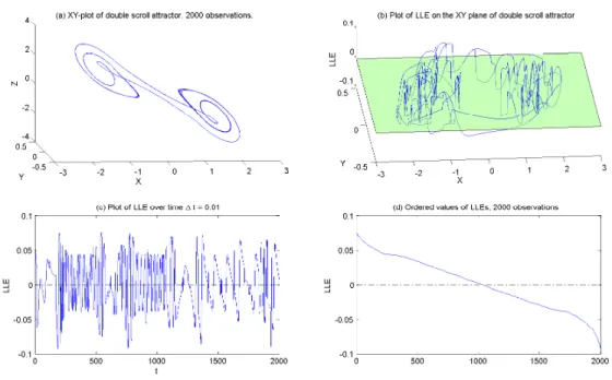
In fact, even “globally chaotic” systems are typically made up of both “chaotic regions", where the LLE is positive, and more stable regions where it is negative [8], as we illustrate in Figures 1, 2 and 3 for the Rössler4, the Lorenz5, and the Chua6 systems, respectively7. In each …gure we display, clockwise from

3_{Other estimations of Lyapunov exponents exist. See, e.g., Gençay [15], Delecroix et al}

[16], Bask and Gençay [17].

4_{We followed the z variable of the following Rössler system:}

8 > < > : dx dt = y z dy dt = x + 0:1y dz dt = 0:1 + z(x 14) ;

with initial values x0= y0= z0= 0:0001and a step size of 0.01, [18]. 5_{We followed the x variable of the following Lorenz system:}

8 > < > : dx dt = 16(y x) dy dt = x(45:92 z) y dz dt = xy 4z ;

with initial values x0= 10, y0= 10and z0= 30, and a step size of 0.01 (Lorenz [19]). 6_{We followed the z variable of the following Chua system:}

8 > < > : dx dt = 9:35(y h(x)) dy dt = x y + z dz dt = 14:286y ;

with h(x) =2₇x ₁₄3(jx + 1j jx 1j) initial values x0 = 0:3, y0= 0:3and z0= 0:28695,

and a step size of 0.01. For an exhaustive gallery of double scroll attractors, see Bilotta et al [20].

the upper left corner: the 3-dimensional attractor in the (x; y; z)-space, the value of the LLE along the orbit ( is displayed on the vertical axis), the value of the LLE along the trajectory, and the distribution of LLE values ranked from highest to lowest. Notice that for each attractor, the value of the LLE takes on positive and negative values (i.e., above and below the = 0 plane depicted in the upper-right corner). Hence, we may expect very stable trajectories where the LLE is small, wheras regions where the LLE is large yield highly unstable behavior.

[FIGURE 1] [FIGURE 2] [FIGURE 3]

3

Solving the selection problem

Assuming that we observe x1; :::; xT, and following the insights of the previous

section, we now investigate conditioning our selection process on the value of the LLE. Formally, our algorithm can be de…ned as follows:

If T , select the "colinear" candidate

otherwise, select the "non colinear" candidate, (2) where is an exogenously given threshold value. We abuse terminology slightly and denote by "colinear" the candidate which maximizes the following scalar product: ^ X_{T +1}c = arg max ^ XT +12C ( ^XT +1 XT) (Xi+1 XT) jj ^XT +1 XTjj jjXi+1 XTjj (3)

where C = f(^x_{T +1}; xT; :::; xT d+2); (^x+T +1; xT; :::; xT d+2)g and Xi+1is the

suc-cessor of the nearest neighbor of XT in phase space. Likewise, we denote by

^ Xnc

T +1, and call "non colinear", the candidate which minimizes the scalar

prod-uct in Expression (3).

In words, the algorithm assumes that when the value of the LLE is low, the orbit is relatively smooth, suggesting that the trajectory to be predicted behaves similarly as the nearest neighbor’s trajectory. Alternatively, when the LLE is "large", the trajectory is considered to behave erratically, so that the trajectory to be predicted is assumed to di¤er from that of its nearest neighbor.

Intuition suggests that one may need to estimate the optimal value of the threshold in terms of prediction accuracy for each chaotic system. Hence, we calculate the mean squared error (MSE) of the predictor using the above

selection algorithm (2) in order to assess which threshold minimizes the MSE: M SEs( ) = 1 n T X t=T n+1 ^ X_ts( ) Xt 2 ; with ^Xs

t( ) = ^Xtc or ^Xtnc according to selection algorithm (2), and where n

is the number of predictions. We compute M SEs_{( ) across all values of in}

the range of the system’s LLE over the last 1000 observations of our sample (n = 1000) using the entire, true information set leading up to the predictee for each prediction. Figure 4 plots the values of M SEs _{as a function of for the}

Rössler, Lorenz and Chua attractors. We …nd that M SEs_{( ) is smallest when}

is the upper bound of the range. In other words, our method seems to not require estimating the optimal threshold, , as one is better o¤ always selecting the colinear candidate and not conditioning the selection process on the LLE, as intuition might have suggested.

[FIGURE 4]

In the remainder of the paper, we shall focus on the performance of ^Xc_{, the}

predictor which systematically selects the colinear candidate. For this predictor, the MSE writes as follows:

M SEc= 1 n T X t=T n+1 ^ X_tc Xt 2 : (4)

Table 1 displays the values of M SEc_{along with the performances of the}

nearest-neighbor predictor: M SEN N = 1 n T X t=T n+1 ^ X_tN N Xt 2 (5)

and of the best of the two possible candidates

M SEb= 1 n T X t=T n+1 min i=c;nc ^ X_ti Xt 2 :8 (6)

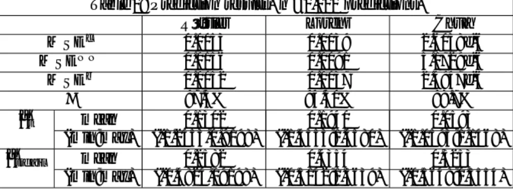
Table 1 also shows the success rate, , in selecting the better of the two can-didate as well as information on the value of the LLE on the orbit (line 6) and information on the LLE on the observations where "wrong" candidate was selected (line 7).

Table 1: Prediction results. n =1,000 predictions. Rössler Lorenz Chua M SEc _{0.0053 0.0039 2.6038e-6} M SEN N _{0.0156 0.0091 5.1729e-6} M SEb _{0.0052 0.0037 2.4947e-6} 97.3% 94.30% 98.7% ^ t mean 0.1302 0.1940 0.0593 (min;max) (-1.2453,0.9198) (-1.4353;1.4580) (-1.0593;1.1468) ^_t jf ail mean 0.2582 0.4354 0.3253 (min;max) (-0.4824,09198) (-0.5142;1.3639) (-0.5648;0.5554) Caption: M SEc, M SEN N and M SEb are as de…ned in (4), (5) and (6). is the selection success rate of the colinear selector. ^t

is the value of the LLE on the 1,000 observations to be predicted. ^

tjf ailis the value of the LLE on the observations where the colinear

selector does not select the best candidate.

For all three systems, we …nd that M SEc _{is substantially smaller than}

M SEN N. Moreover, M SEc is relatively close to M SEb, suggesting that our procedure selects the best of the two candidates quite often. In fact, on all three attractors, we obtain success rate, , close to 100%. Finally, on the few predictions where our predictor does select the "wrong" candidate, the value of the LLE is relatively high compared to the average LLE on the attractor (0.25 versus 0.13 for Rössler, 0.44 versus 0.19 for Lorenz, and 0.33 versus 0.06 for Chua) These …ndings are consistent with the intuition that prediction is more di¢ cult in regions of the attractor which are more sensitive to initial conditions. While this …nding seems to con…rm that the value of the LLE plays a small role in the selection problem, recall that our results show that conditioning selection on the value of the LLE would not lead to improved predictions, as measured by M SEs_{( ).}

4

Forecasting

In this section, we detail the role of the value of the LLE on the size of errors and on the performance of the selection procedure as well as the performance of the predictor in the short and medium run.

4.1

Role of the LLE on error size

The following tables show the success rates of the selection procedure of ^Xc_and

the resulting MSE broken down in small value intervals for the LLE. Doing so allows one to assess how the performance of the procedure and of the predictor depends on the (local) chaoticity of the region considered. represents the

ratio of the number of times the best candidate was selected over the number of predictions in the interval considered. These predictions are then broken down into the number of good selection (nsucc) and the number of failures to

select the best candidate (nf ail). Next, M SEc shows the mean squared error

of our predictor (using colinear selection) on each interval. M SEc_{jsucc. and}

M SEc_{jfail show the value of MSE}c _{considering only the predictions where}

the best candidate was correctly and incorrectly selected, respectively. Finally, M SEN N _{displays the mean squared error of the nearest neighbor predictor on}

the relevant interval.

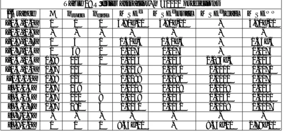
Table 2: Rössler attractor, n =1000 predictions

^_{t range nsucc nf ail M SE}c _{M SE}c_{jsucc M SE}c_{jfail M SE}N N

[-1.3,-1.1] 1 1 0 3.91e-11 3.91e-11 - 3.91e-11

[-1.1,-0.9] - - -

-[-0.9,-0.7] 1 5 0 1.32e-6 1.32e-6 - 1.34e-6 [-0.7,-0.5] 1 68 0 0.0073 0.0073 - 0.0073 [-0.5,-0.3] 0.98 106 2 0.0033 0.0033 2.096e-5 0.0034 [-0.3,-0.1] 0.97 105 3 0.0059 0.0060 0.0001 0.0072 [-0.1,0.1] 0.98 125 3 0.0089 0.0091 0.0000 0.0176 [0.1,0.3] 0.97 149 4 0.0019 0.0019 0.0009 0.0054 [0.3,0.5] 0.97 222 8 0.0059 0.0056 0.0132 0.0101 [0.5,0.7] 0.97 192 6 0.0051 0.0052 0.0009 0.0127 [0.7,0.9] - - -

-[0.9,1.1] 0 0 1 9.34e-10 - 9.34e-10 2.79e-11 Caption: Each row relates to observations Xtfor which the LLE belongs to ^t

range. is the selection success ratio (1=100%). nsuccand nf ailare the number

of predictions for which the colinear selector selects correctly and incorrectly, respectively. M SEc _{and M SE}N N _{are as de…ned in (4) and (5). M SE}c_jsucc

and M SEc_{jfail correspond to MSE}c_{restricted to the previously de…ned n} succ

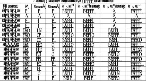
Table 3: Lorenz attractor, n =1000 predictions

^_{t range nsucc. nf ail. M SE}c _{M SE}c_{jsucc: M SE}c_{jfail: M SE}N N

[-1.5,-1.3] 1 1 0 0.0001 0.0001 - 0.0001 [-1.3,-1.1] - - - -[-1.1,-0.9] 1 3 0 0.0016 0.0016 - 0.0016 [-0.9,-0.7] 1 3 0 0.0013 0.0013 - 0.0013 [-0.7,-0.5] 0.99 67 1 0.0033 0.0034 0.0003 0.0035 [-0.5,-0.3] 0.99 92 1 0.0049 0.0049 0.0000 0.0054 [-0.3,-0.1] 0.98 98 2 0.0056 0.0054 0.014 0.0098 [-0.1,0.1] 0.93 108 8 0.0038 0.0039 0.0026 0.0052 [0.1,0.3] 0.94 109 7 0.0041 0.0036 0.011 0.0077 [0.3,0.5] 0.96 195 8 0.0021 0.0020 0.0049 0.0088 [0.5,0.7] 0.91 223 22 0.0044 0.0038 0.0102 0.0079 [0.7,0.9] 0.90 18 2 0.0011 0.0008 0.0033 0.0012 [0.9,1.1] 0.81 13 3 0.0006 0.0003 0.0016 0.0016 [1.1,1.3] 0.82 9 2 0.0034 0.0031 0.0047 0.0027 [1.3,1.5] 0.80 4 1 0.042 0.052 0.0019 0.0015 Caption: Each row relates to observations Xtfor which the LLE belongs to

^

t range. is the selection success ratio (1=100%). nsucc and nf ail are the

number of predictions for which the colinear selector selects correctly and incorrectly, respectively. M SEc _{and M SE}N N _{are as de…ned in (4) and (5).}

M SEc_{jsucc and MSE}c_{jfail correspond to MSE}c _{restricted to the previously}

de…ned nsucc and nf ail observations, respectively.

Notice that for all three attractors the size of errors is relatively stable over the range of LLEs when selection is successful. This indicates that our method accurately corrects for the dispersion of neighboring trajectories as measured by the value of the LLE. If this were not the case, one would expect the MSE to increase monotonically with the value of LLE. In fact, errors become large only for values of the LLE near the upper end of their range (above 0.9 for the Rössler attractor, above 1.1 for the Lorenz attractor, and above 0.5 for the Chua attractor). A possible reason for this sudden increase may be that our estimator for the value of the LLEs is not su¢ ciently robust in regions of high chaoticity. We expect that a more sophisticated estimation method for the LLE may solve this issue, which we address in a companion paper.

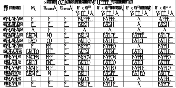
Table 3: Chua attractor, n =1000 predictions

^_{t range nsucc. nf ail. M SE}c _{M SE}c_{jsucc. M SE}c_{jfail: M SE}N N

( 10 4_{) ( 10} 4_{) ( 10} 4_{) ( 10} 4₎ [-1.3,-1.1] 1 1 0 0.3111 0.3111 - .3111 [-1.1,-0.9] 1 1 0 0.1765 0.1765 - 0.1765 [-0.9,-0.7] - 0 0 - - - -[-0.7,-0.5] 0.9873 78 1 0.0376 0.0381 0.0002 0.0391 [-0.5,-0.3] 0.98 98 2 0.0339 0.0332 0.0686 0.0362 [-0.3,-0.1] 1 116 0 0.0218 0.0218 - 0.0244 [-0.1,0.1] 0.9918 241 2 0.0074 0.0072 0.0285 0.0241 [0.1,0.3] 0.9917 120 1 0.0097 0.0097 0.0124 0.0228 [0.3,0.5] 0.9884 171 2 0.0199 0.0199 0.0183 0.0221 [0.5,0.7] 0.9740 150 4 0.0553 0.0508 0.2261 0.0239 [0.7,0.9] 0.8750 7 1 0.1333 0.0721 0.5619 0.0981 [0.9,1.1] 1 2 0 0.0884 0.0884 - 0.0025 [1.1,1.3] 1 2 0 0.2440 0.2440 - 0.0091 Caption: Each row relates to observations Xtfor which the LLE belongs to

^_{t range. is the selection success ratio (1=100%). nsucc and nf ail are the} number of predictions for which the colinear selector selects correctly and incorrectly, respectively. M SEc _{and M SE}N N _{are as de…ned in (4) and (5).}

M SEc_{jsucc and MSE}c_{jfail correspond to MSE}c _{restricted to the previously}

de…ned nsucc and nf ail observations, respectively.

Notice that for the Rössler attractor, for most values of the LLE, the size of errors when failing to select is on average less than when selecting accurately. For example, for ^ 2 [0:5; 0:7], MSEcjsucc = 0:0052 > 0:0009 = M SEcjf ail.This

apparently surprising observation is actually encouraging as it indicates that selection mistakes occur mostly when there is little need for correction. Such situations may arise because XT’s nearest neighbor is very close to XT or,

alternatively, when both candidates, ^x_{T +1}and ^x+_{T +1}are both very close to xi+1

due to space orientation considerations. The same phenomenon can be observed for the Lorenz system up to ^ = 0:1 and for ^ > 1:3, but is less systematic for the Chua system.

Regarding the selection accuracy, as measured by , we …nd that our algo-rithm selects almost perfectly for all three attractors, and in most ranges of ^. As expected, dips slightly for larger values of ^ in the case of the Rössler and Lorenz attractors, which is in line with the common intuition according to which trajectories are more stable, or smoother, where the value of the LLE is small and more irregular for large values of the LLE. Surprisingly, the Chua attractor behaves somewhat di¤erently. Interestingly, selection mistakes occur on all at-tractors for negative values of the LLE, where the system is supposedly locally "stable". Hence, our results suggest that the focal value of = 0, traditionally separating order from chaos, bears little meaning in terms of forecasting.

4.2

Forecasting several steps ahead

We now explore the possibility of forecasting a chaotic time series several steps ahead using our correction method. In order to make predictions h-steps ahead, we proceed iteratively, including the successive one-step predictions.9

In addition to extending our predictions to several steps ahead, we jointly investigate the role of the number of neighbors to consider in the prediction and in the estimation of the LLE. We estimated the LLE using Wol¤’s [6] algorithm with in…nite bandwith and k neighbors, and applied our correction method to the average of the images of these neighbors (k NNP).

4.2.1 Rössler attractor

The following table shows M SEc _{and M SE}N N _{as a function of the number}

of neighbors and the prediction horizon in the top and bottom half of the ta-ble, respectively. For each column, and for each predictor, the numbers shown in bold are the smallest mean squared error for each horizon. Therefore, the corresponding number of neighbors, k, is optimal for that horizon.

Rössler attractor h = 1 h = 2 h = 6 h = 7 h = 10 k = 1 0.0053 0.0117 0.1889 0.3107 0.8575 k = 2 0.0045 0.0144 0.2901 0.4890 1.6762 k = 3 0.0058 0.0184 0.2114 0.3212 0.8501 k = 4 0.0077 0.0240 0.3074 0.4301 1.3332 k = 5 0.0091 0.0278 0.3650 0.5193 1.1830 k = 10 0.0103 0.0412 0.6380 0.9228 2.2703 k = 20 0.0283 0.1178 1.8714 2.7681 6.4980 M SE1 N N 0.0156 0.0315 0.2392 0.3402 0.7928 M SE2 N N 0.0194 0.0384 0.2229 0.3017 0.6318 M SE3 N N 0.0228 0.0485 0.2784 0.3710 0.7410 M SE4 N N 0.0242 0.0560 0.3513 0.4711 0.9528 M SE5 N N 0.0295 0.0684 0.4224 0.5623 1.1133 M SE10 N N _{0.0500 0.1306 0.9188 1.2228 2.3539} M SE20 N N _{0.1247 0.3282 2.2649 2.9775 5.4714}

Caption: The top and bottom half of the table display M SEc _{and M SE}N N

as a function of the number of neighbors k and the prediction horizon, h; respectively.

As expected, predictions are more accurate in the shorter run. Moreover, increasing the number of neighbors, k, generally seems to decrease the accu-racy of the prediction. Note that this is also true for the uncorrected

nearest-9_{For instance, ^X}

t+2is obtained by constructing the (estimated) history (X1; :::; Xt; ^Xt+1).

Next, ^Xt+3 is obtained via history (X1; :::; Xt; ^Xt+1; ^Xt+2), and so on. Hence,no further

neighbor predictor. Finally, our correction method improves upon the uncor-rected nearest-neighbor predictor up until six steps ahead.

4.2.2 Lorenz attractor Lorenz attractor h = 1 h = 2 h = 7 h = 8 h = 10 k = 1 0.0039 0.0176 0.6821 1.0306 1.9406 k = 2 0.0024 0.0102 0.4151 0.6249 1.2429 k = 3 0.0020 0.0081 0.3387 0.5103 0.9955 k = 4 0.0014 0.0057 0.2873 0.4347 0.8803 k = 5 0.0014 0.0061 0.3179 0.4852 0.9724 k = 10 0.0016 0.0071 0.3374 05124 1.0329 k = 20 0.0021 0.0101 0.4322 0.6474 1.2333 M SE1 N N _{0.0091 0.0246 0.3485 0.4877 0.8730} M SE2 N N _{0.0084 0.0226 0.2994 0.4152 0.7318} M SE3 N N _{0.0081 0.0220 0.2951 0.4087 0.7181} M SE4 N N _{0.0086 0.0231 0.2974 0.4096 0.7133} M SE5 N N _{0.0091 0.0243 0.2991 0.4104 0.7123} M SE10 N N _{0.0129 0.0349 0.3775 0.5001 0.8136} M SE20 N N _{0.0207 0.0562 0.5397 0.6893 1.0423}

Caption: The top and bottom half of the table display M SEc _{and M SE}N N

as a function of the number of neighbors k and the prediction horizon, h; respectively.

Here also, predictions are more accurate in the shorter run. However, unlike for the Rössler attractor, the simulation results suggest that accuracy increases with k up to a point (k = 4). Beyond that, increasing the number of neighbors is detrimental to the accuracy of the method (except for h = 20, which is too large a horizon for our predictions to be trusted).

As is the case with the Rössler attractor, our method performs uniformly better than the corresponding uncorrected nearest-neighbor predictor for hori-zons of up to seven steps ahead.

4.2.3 Double scroll attractor

Chua double scroll

h = 1 h = 2 h = 3 h = 5 h = 10 k = 1 2.6038e-6 1.1247e-5 3.2935e-5 1.3694e-4 0.0012 k = 2 1.6569e-6 5.5148e-6 1.5541e-5 6.1758e-5 5.5566e-4 k = 3 1.5344e-6 5.6257e-6 1.5912e-5 6.3038e-5 6.1618e-4 k = 4 2.0762e-6 6.9228e-6 1.9519e-5 7.4392e-5 6.7625e-4 k = 5 2.6426e-6 8.7472e-6 2.3965e-5 8.7017e-5 6.6244e-4 k = 10 4.4688e-6 1.7896e-5 5.2198e-5 1.9949e-4 0.0014 k = 20 6.4272e-6 2.7342e-5 9.3183e-5 4.4513e-4 0.0042

M SE1 N N _{5.1729e-6 8.7554e-6 1.6178e-5 5.2720e-5 4.8311e-4}

M SE2 N N _{4.3528e-6 7.9723e-6 1.5174e-5 4.9276e-5 4.3521e-4}

M SE3 N N _{5.9985e-6 1.1757e-5 2.2003e-5 6.4616e-5 4.7283e-4}

M SE4 N N _{8.6114e-6 1.7168e-5 3.1539e-5 8.6965e-5 5.6469e-4}

M SE5 N N _{1.1190e-5 2.3201e-5 4.2647e-5 1.1362e-4 6.7550e-4}

M SE10 N N _{1.7453e-5 4.5731e-5 9.4048e-5 2.6532e-4 0.0014}

M SE20 N N _{5.5861e-5 1.6005e-4 3.3975e-4 9.4208e-4 0.0042}

Caption: The top and bottom half of the table display M SEc _{and M SE}N N

as a function of the number of neighbors k and the prediction horizon, h; respectively.

Again, we see that our prediction results improve upon those of the corre-sponding uncorrected k-nearest-neighbor predictor, but only in the very short run (up to h = 2). Also, as was the case with the other systems, the opti-mal number of neighbors is low: k = 2. Beyond that number, any information carried by neighbors farther away seems to only pollute the prediction results

5

Concluding comments

We further developed the methodology on using the information contained in the LLE to improve forecasts. Our contributions are threefold. First, the selection problem raised in [1] is no longer an issue, and does not require conditioning candidate selection on the value of the LLE. Next, our results con…rm that it is indeed possible the LLE to improve forecasts, and highlight an interesting fact: the focal value of = 0, which traditionally separates order from chaos, does not play any role in the forecasting of chaotic systems. In other words, our methodology performs equally well on both stable and chaotic regions of the attractors studies. Finally, we examined the sensitivity of our methodology to varying the number k of neighbors as well as of the step-ahead horizon, h. While our goal was not to determine the optimal number of neighbors to consider for forecasting, it seems that each attractor admits a rather low optimal number of neighbors. We have worked with a …xed embedding dimension, d, throughout.

Now that we have ascertained the validity of the approach, the next step is to con…rm its performance on real physical or …nancial data.

References

[1] D. Guégan, J. Leroux, Forecasting chaotic systems: The role of local Lya-punov exponents, Chaos, Solitons and Fractals, 41 (2009a) 2401-2404. [2] D. Guégan, J. Leroux, Local Lyapunov Exponents: A New Way to

Pre-dict Chaotic Systems, forthcoming in Topics on Chaotic Systems: Selected papers from CHAOS 2008 International Conference, World Scienti…c Eds., 2009b.

[3] D. Murray, Forecasting a chaotic time series using an improved metric for embedding space, Physica D, 68 (1993) 318-325.

[4] R. Doerner, B. Hübinger, W. Martienssen, S. Grossman, S. Thomae, Pre-dictability Portraits for Chaotic Motions, Chaos, Solitons and Fractals, 1 (1991) 553-571.

[5] H.D.I. Abarbanel. Local and global Lyapunov exponents on a strange at-tractor. Nonlinear Modeling and Forecasting, SFI Studies in the Science of Complexity, Casdagli M and Eubank S Eds, Addison-Wesley, 1992; Proc. Vol. XII: 229-247.

[6] R.C.L. Wol¤, Local Lyapunov exponents: looking closely at chaos. Journal of the Royal Statistical Society B, 54 (1992) 353 –371.

[7] B. Eckhardt, D. Yao, Local Lyapunov exponents in chaotic systems, Phys-ica D, 65 (1993) 100-108.

[8] B. Bailey, Local Lyapunov exponents: predictability depends on where you are. Nonlinear Dynamics and Economics, Kirman et al. Eds, 1997. [9] J.D. Farmer, J.J. Sidorowich, Predicting chaotic time series. Physical

Re-view Letters, 59 (1987) 845 –848.

[10] C. Ziehmann, L.A. Smith, J. Kurths, Localized Lyapunov exponents and the prediction of predictability. Physics Letters A, 271 (2000) 237-251. [11] M. Shintani, O. Linton, Nonparametric neural network estimation of

Lya-punov exponents and a direct test for chaos, 120 (2004) 1-33.

[12] D. Guégan, L. Mercier, Stochastic and chaotic dynamics in high-frequency …nancial data. Signal Processing and Prediction, Prochazka Eds, 1998; 365-372.

[13] J.P. Eckmann, D. Ruelle, Ergodic theory of chaos and strange attractors. Review of Modern Physics, 57 (1985) 615-656.

[14] F. Takens, Estimation of dimension and order of time series. Progress in Nonlinear Di¤erential Equations and their Applications, 19 (1996) 405-422. [15] R. Gencay, A statistical framework for testing chaotic dynamics via

Lya-punov exponents, Physica D, 89 (1996) 261-266.

[16] M. Delecroix, D. Guégan, G. Léorat, Determining Lyapunov exponents in deterministic dynamical systems, Computational Statistics and Data Analysis, 12 (1997) 93-107.

[17] M. Bask, R. Gençay, Testing chaotic dynamics via Lyapunov exponents, Physica D, 114 (1998) 1-2.

[18] D. Guégan, Les Chaos en Finance: Approche Statistique. Economica Eds.; 2003, 420 pp.

[19] E.N. Lorenz, Deterministic non-periodic ‡ow. Journal of Atmospheric Sci-ence, 20 (1963) 130-141.

[20] E. Bilotta, G. Di Blasi, F. Stranges, P. Pantano, A Gallery of Chua Atrac-tors. Part VI. International Journal of Bifurcation and Chaos, 17 (2007) 1801-1910.

-1.5 -1 -0.5 0 0.5 1 1.5 0.005 0.01 0.015 0.02 0.025 0.03 0.035 T hreshold M ean s quar ed e rr or

(a) Rös sler system

-1.50 -1 -0.5 0 0.5 1 1.5 0.005 0.01 0.015 0.02 0.025 0.03 T hreshold M ean s quar ed e rr or (b) Lorenz s ys tem -1.52 -1 -0.5 0 0.5 1 1.5 3 4 5 6 7 8 9 10 11 12x 10

- 6 (c) Chua double scroll

T hreshold M ean s quar ed e rr or MSE MSE (NN) MSE (Best)