The risk and return of venture capital

(1)

1

The risk and return of venture capital

Historical return, alpha, beta and individual performance

drivers (1983-2009)

Stéphane Koch

1

April 2014

Abstract

We analyse the returns and the risk profile of venture capital based on a sample of 1,953 funds raised between 1983 and 2009. In a historical perspective, we first show that the strong returns during the dotcom era are followed by a decrease and a convergence of returns. However, we find strong evidence of outperformance compared to public markets, with a PME of 1.26 (vs. S&P500) and 1.08 (vs. Nasdaq). In a second time and in order to assess the risk profile and the risk-adjusted returns of venture capital, we focus on the beta and alpha of this asset class. Beta stands between 1.0 and 1.8 and the quarterly CAPM alpha between 0.3%-5.1%, revealing a clear positive risk-adjusted performance. Lastly, we focus on individual fund characteristics as potential drivers of performance. If we find no evidence of size driving overall returns, we show that location (US) is a strong determinant of performance. Stage-focus does not influence returns, unless the fund is a general fund, in which case returns are driven downwards. Finally, we confirm the negative relationship between IRR and duration, and show that funds whose payback period is shorter are likely to outperform.

Keywords: venture capital, private equity, performance, return.

Acknowledgements: I would like to first thank Mr. Christophe Spaenjers for supervising this research paper. I am also very grateful to Mr. Amaury Bouvet for helping me to understand the different databases and collect data.

1

(2)

2

1 Introduction

This paper examines the performance of venture capital as an asset class. By definition, venture capital is a component of private equity, the act of investing in the equity of a private, non-listed, company. Among private equity, venture capital funds seek returns by investing in young companies whereas buyout funds target mature and established companies. Despite the dramatic growth in private equity investments over the last twenty years, the very basic characteristics of venture capital remain controversial: if an extensive research already exists on the subject, the studies have reached different findings and no consensus exists on questions such as the risk and return of this asset class. For Gompers and Lerner (2000), the risk-return profile is precisely “what we don’t know about venture capital”.

The main goal of this paper is therefore to get a better understanding of the returns of the venture capital asset class. First, what is the historical performance of venture capital investments, and how this performance compares to public equities? Do they yield larger risk-adjusted returns than publicly traded securities? The existing research emphasizes the different cycles in the performance of venture capital, with increasing returns for funds raised in the 80s and the 90s (Ljungqvist and Richardson (2003)) and a reversed pattern after 1999 and the Internet bubble (Harris, Jenkinson and Kaplan (2013)), however the average return during these cycles and whether or not funds have outperformed public markets remains controversial. Second, we would like to understand the specificity of venture capital investments and therefore estimate the alpha and beta of such investments1. From a theoretical standpoint, the illiquidity of such investments in private companies should lead to a premium and consequently to high returns in comparison to the overall market. Moreover, venture capital firms often keep around two percent of the invested capital (see Gompers and Lerner (1999), Lerner, Schoar and Wongsunwai (2007)) to compensate for their monitoring role within portfolio companies, which should normally result in a high performance (Admati and Pfleiderer (1994)). Finally, we would like to characterize the type of fund which outperforms and underperforms in terms of size, geography and stage specialisation. This will be the last focus of this paper.

1_{The beta, defined more precisely later in this paper, represents the degree of correlation between an asset and} the overall market. The alpha measures how effectively an asset has outperformed or underperformed the theoretical performance. It depends on the model used to forecast asset returns.

(4)

4

1.1 Why the performance of venture capital funds matters

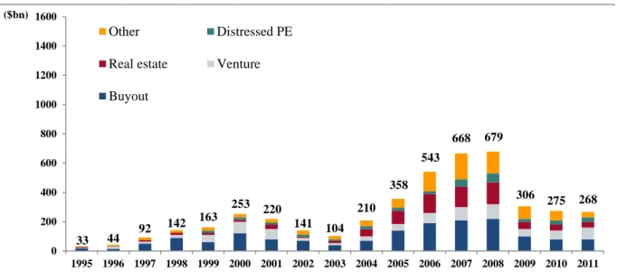
The private equity asset class, made mainly of buyout and venture capital funds, has grown importantly since 1990, with institutional investors dedicating more and more capital to private equity in their tactical allocation. A good example is given by the Harvard endowment, allocating 0% to private equity in 1980, 7% in 1984 and 16% in 20131. Within this asset class, venture capital has increased significantly as well, from $3bn flowing into venture funds in 1990 to around $100bn in 2012. Venture capital has consequently been the fastest growing segment among private equity, with a 1995-2011 CAGR of 20%.

Figure 1: Global private equity capital raised by fund type

Source: “Global Private Equity Report”, Bain & Company, p.25.

One of the reasons of the success of the private equity segment among asset managers is probably its hedging property. Many invest heavily in private equity with the belief that the returns of private equity investments are largely uncorrelated with public markets and business cycles. As an example, the Yale endowment reports that such funds “can generate incremental returns independent of how the broader market will be performing2”, something interesting given the current context in public markets. This belief, discussed later in this paper, has already received attention from previous research. According to Gottschalg, Phalippou and Zollo (2003), the performance of venture funds strictly follows business cycles and consequently the beta for such investments should be around one, as documented by Lerner and Schoar (2005).

1_{“Harvard Management Company”, An evolving view of asset classes: Creating the optimal mix of investments.} 2

The Yale Endowment 2010.

33 44 92 142 163 253 220 141 104 210 358 543 668 679 306 275 268 0 200 400 600 800 1000 1200 1400 1600 1995 1996 1997 1998 1999 2000 2001 2002 2003 2004 2005 2006 2007 2008 2009 2010 2011 ($bn) Other Distressed PE

Real estate Venture

(5)

5 Moreover, venture capital is interesting from a macro perspective. It enables young and innovative companies to receive financing from outside investors to finance their growth. Given the uncertain prospects, it is difficult for start-ups to receive bank financing and venture capital can often be an efficient way to grow and professionalize young companies, as evidenced by Hellman and Puri (2002). A company like Sequoia Capital, one of the biggest venture capital firms specialized in technology companies, has helped Cisco, Nvidia, Apple or Youtube grow and become strong established companies. According to Hege and Palomino (2003), the strong economic growth in the US in comparison to Europe can partly be attributable to the emphasis put on venture capital and contractual differences such as the greater use of control rights. It is therefore clear that venture capital plays an important role as a catalyst for economic growth and knowing more about the risk and return of these investments is of primary importance.

1

.2

Overview of the research paper

In this paper, we analyse the performance of funds based on the IRR measure traditionally used in private equity. However, this measure is imperfect for at least two reasons, described into more details in section 3. Firstly, it assumes that all the proceeds are reinvested at the IRR, which of course is not the case. Secondly, it does not take into account the return on public markets. Bradley, Mulcahy and Weeks (2012) recommend “rejecting performance marketing narratives that anchor on internal rate of return” and “adopt public market equivalent as a consistent standard for VC performance reporting” instead. This is why we build another measure, the public market equivalent (PME), based on the methodology developed by Kaplan and Schoar (2005). This metric compares the return one gets by investing all the money into the fund, basically the IRR, and the return obtained by investing everything into public markets, using for example the return of the S&P500.

This paper answers three questions that previous research has not answered yet or for which there is not a clear consensus: firstly, whether venture capital funds have historically outperformed public equities and whether its performance help justify the dramatic growth of this asset class; secondly, define the alpha and beta of this asset class; finally, whether size, geography and stage specialisation are explanatory variables of a fund performance.

We show that historically venture capital funds have yielded an average IRR of 9% and have significantly outperformed public markets, with a PME of 1.26 using the S&P500 and 1.08 using the Nasdaq Composite index. Especially, funds raised between 1993 and 1996

(6)

6 have had a very strong performance. However, it seems that the overall performance of VC funds is being less and less volatile and is converging both in the US and Europe, because of a maturing market.

Using three different venture capital indices from VentureXpert, Cambridge Associates and Sand Hill Econometrics, we estimate the beta and alpha of venture capital. We also test for sensitivities using two benchmarks: the S&P500 index and the Nasdaq Composite Index. We find that the beta lies between 1.0 and 1.8, close to the findings of previous literature. This result is consistent with both the S&P500 and the Nasdaq Composite Index and proves that venture capital tends to overreact to public markets. However, this beta is calculated using lagging market returns, which shows that venture capital returns are linked to current and past market returns. We document a positive quarterly alpha between 0.3% and 5.1% revealing a strong risk-adjusted return for venture capital.

Finally, we find evidence that location can be considered as a performance driver. Funds in the US significantly outperform European funds. Additionally, we confirm the theoretical negative relationship between the lifetime of a fund and its return, suggesting for practitioners to focus on general partners showing a strong ability to exit investments quickly. However, this conclusion is to be mitigated by the difference between US and Europe, where this relationship is weaker. Eventually, if non-specialized funds slightly underperform the venture capital industry, stage specialisation and size have little explanatory power over the return of a fund.

The rest of the paper proceeds as follow. Section 2 provides some theoretical background on venture capital, describing the typical structure of a private equity investment. Section 3 surveys and summarizes the relevant literature. In section 4, we present our research questions and lay out our hypotheses. Section 5 presents the dataset obtained from VentureXpert and warns the reader about potential biases. It also describes the variables that will be used in our empirical analysis. Section 6 presents the key findings of the empirical analysis. Section 7 concludes.

(7)

7

2 Theoretical background on venture capital

2.1 The emergence of venture capital

Gompers (2004) situates the emergence of venture capital in the early 80s in the US, after changes in the Employee Retirement Income Security Act (ERISA). Before, this act largely prohibited pension funds from allocating large amounts of money to high-risk assets including venture capital. After 1979, they were allowed to invest up to 10% of their capital into venture funds.

However, as early as the 19th century, the ancestors of venture capital began to look for risky, high-return investments in diverse industries, as described by David Lampe and Susan Rosegrant: “The city’s great fortunes, including those of the Vanderbilts, Whitneys, Morgans and Rockefellers, were based on such ventures as railroads, steel, oil and banking. Although not all investors were so well-known, it was wealthy families such as these that bankrolled Boston’s earliest high tech entrepreneurs. When the young Scot Alexander Graham Bell needed money in 1874 to complete his early experiments on the telephone, for example, Boston attorney Gardiner Green Hubbard and Salem leather merchant Thomas Sanders helped out, and later put up the capital to start the Bell Telephone Co. in Boston”1.

After the 80s, venture capital became more and more important and reached a peak at the end of the 90s with the high-tech bubble. It is documented that even some buyout funds allocated part of their investments to start-ups during this period.

2.2 Types of private equity investments

Private equity is made of 5 main classes: venture capital, growth capital, mezzanine financing, leveraged buyout and distressed buyouts, investing at distinct stages of development:

 Venture capital firms typically invest in start-ups at an early stage of development with a negative cash-flow generation. The investment is generally a minority stake characterized as high-risk/high-return.

 Growth capital is made of equity or debt investments in growing companies that require additional financing for their working capital, capital expenditures or acquisitions.

1

(8)

8  Mezzanine funds invest in mezzanine debt or preferred equity, i.e. all the instruments

between traditional equity and senior debt on the balance sheet.

 Leveraged buyout (LBO) is the biggest class among private equity. LBO funds seek returns from the acquisition of mature companies with a significant amount of debt or borrowed funds.

 Distressed buyout funds purchase distressed companies below market value looking for example for a corporate restructuring.

A private equity firm is generally specialized into one of these investment strategies. Moreover, there is often a geographical focus, either at a country (United States) or a regional level (Western Europe, South-East Asia, etc.) as well as an industry focus (real estate, retail, healthcare, technology, media & telecom, etc.).

2.3 Private equity investment structure and definition of terms

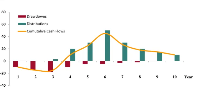
A private equity firm, known as the general partner (GP), is traditionally made of several investment teams raising capital from outside investors, the limited partners (LPs). Limited partners are typically endowments, pension funds, high net worth individuals or any other type of institutional investor. Once the fund is created, the GP is the manager, whereas LPs are only passive investors. In this paper, we will call capital commitment every amount of money flowing from a limited partner to the fund, basically the amount of money that investors have agreed to subscribe to the fund. It is important to note that the capital is flowing to the fund only once the GP has found an interesting project to invest in. Consequently, the committed capital is gradually invested into different projects, what we define as a draw-down. The capital committed that the fund has not drawn down is called undrawn commitment whereas the part invested by the fund is characterized as assets under management. The sum of these two items – assets under management and undrawn commitments – minus the net debt1 used for financing gives the net asset value. The GP is required to invest the capital generally between 3 to 5 years and has then another 5 to 7 years to exit its investment and give back the money to the LPs, what we call a distribution.

A private equity investment is therefore nothing else than a stream of cash inflows and cash outflows, usually described as the “J-curve”. The J-curve is precisely what makes the valuation of private equity investments difficult, as we need to estimate the whole net asset

1

(9)

9 value at any point in time, or every quarter as reported by VentureXpert, which means knowing the value of the undrawn and the invested capital. The actual return is known only at exit, when the fund is liquidated and when we can observe the cash-flows that are given back to investors.

Figure 2: J-curve description

Source: “Investment Banking: Valuation, Leveraged Buyouts, and Mergers & Acquisitions”, J. Rosenbaum and J. Perella, John Wiley &

Sons, 2009.

To remunerate the general partner for its expertise and management of investments, venture capital firms generally charge a 2% interest based on asset under management. Then, if the fund has reached a minimum return known as the hurdle rate, generally 8%, it takes an additional 20% performance fee called carried interest from exited investments (Gompers and Lerner (1999), Lerner, Schoar and Wongsunwai (2007)). Figure 3 below should clarify the traditional fee structure of any private equity firm.

2.4 Overview of venture capital funds

Actors in the venture capital landscape are extremely diversified. First, venture capital funds are bigger in the United States than somewhere else and the industry is somehow maturing. In Europe and Asia, the industry is growing importantly and venture capital is still much less established than in the US. Structural differences also exist between the US and Europe, such as “the more frequent use of convertibles in the US and the replacement of the entrepreneur”, as studied by Hege, Palomino and Schwienbacher (2003).

-40 -20 0 20 40 60 80 1 2 3 4 5 6 7 8 9 10 Year Drawdowns Distributions

(10)

10 Figure 3: Private equity fee structure

Source: 3i 2007 annual report.

Differences also appear in the specialisation, with firms focusing on different stages. The first stage in VC investing is seed, targeting companies with not yet established operations. The next stage is the early stage for companies able to begin operations but needing to boost sales. Finally, the late stage provides capital to well-established companies generally before an initial public offering.

3 Literature review

In this section, we review the existing literature about the performance of venture capital funds, keeping in mind the 3 objectives of this paper:

 Understand the average historical performance of venture capital and determine whether or not this asset class has outperformed public markets.

 Study the risk-adjusted return of venture capital, focusing on the alpha and beta of this asset class.

 Focus on individual characteristics of funds such as size, geographic focus and stage specialisation and see how they help explain the overall performance of a fund.

Company A Carried interest

Company B Management fee

Company C Cash returned to investors

Company D Company E

£10m

1. A £100m fund invests in 2. Assume £200m cash received by investors 3. Assume the fund is exited after 10 years 5 companies by the end of the fund, i.e. when companies * Management fees of 1% per year = 10m

are sold * Carried interest = 20% x profit = 20% x (100m - 10m) = £18m £100m £200m £200m £172m £18m

(11)

11 We have focused primarily on papers which analyse the performance at a fund level, which corresponds to our approach, some research studying the return of each investment. Moreover, all the data below is net of fees, i.e. after management fees and carried interest have been paid out to the fund. Beyond our three questions, a first part will be dedicated to performance measurement. The two last subsections will deal with the persistence in performance and the problem of success bias in the sample selection.

3.1 How to measure the performance of a private equity investment

The first measure one naturally think about when speaking of private equity is the internal rate of return (IRR), as this is the most commonly used measure in this industry. By definition, the internal rate of return is the discount rate that makes the net present value of a stream of cash flows equal to zero, i.e.:

In the case of a private equity investment and referring to the previously described J-curve, the equation looks like:

where Draw represents the draw-downs from the LPs to the fund and Dist the distributions from the fund to the GP. Here, the investment period is 2 years and the fund exits the investments after n years.

The advantage of the IRR measure is its simplicity. However, the IRR implicitly assumes that all the cash flows distributed to LPs have been reinvested at the same rate (Gottschalg, Phalippou and Zollo (2003), Jagannathan and Sorensen (2013)). For example, if a fund has a return of 40% and distributed half of the cash very early in the investment life, this number assumes that the amount of money distributed early has been reinvested at a rate of 40% as well, which is very unlikely. This is the reason why it is difficult to compare several investments with the same IRR and a different duration.

The solution brought by Gottschalg and Phalippou is the modified IRR (MIRR) which assumes a fixed rate at which distributions are reinvested, rather than the IRR itself. In their study of 1,184 funds raised between 1980 and 1995, they show that the top-performing fund

(12)

12 has an unrealistic IRR of 464% and an M-IRR of 31% using a fixed rate of 8%. Therefore, IRRs can be misleading when comparing the performance of funds, in addition to skewing the performance of “star” funds.

However, there is a second issue with the IRR: as an absolute measure, it does not adjust for the market return, contrary to the CAPM equation, for instance. A new measure, the public market equivalent (PME), was introduced by Long and Nickels (1996) and has then been refined by Kaplan and Schoar (2005). The idea is to compare the IRR of the fund with the IRR the investor would have got by investing all the commitments in the S&P500, for instance. According to the definition of terms, if and respectively denote the distribution from the fund to the LPs and the capital calls from the LPs to the fund at time t, and is the realized market return (from the S&P500, for example) from the inception of the fund to the time of the distribution or the capital call, then PME is defined as:

∑ ∑

As an illustration, a PME of 1.03 means the fund has returned 3% more than public markets over the investment period. You can refer to the numerical example below for a comparison between these three performance measures.

In this example, we suppose that the fund manages to raise $100m from diverse limited partners. It invests these $100m successively during the first 2 years: $60m are invested directly, $20m are invested during year one (for simplicity about discount rates, we suppose that this amount is invested at the end of the year) and finally $20m are invested at the end of year 2. These investments generate distributions (in the form of cash-flows or shares) from year 2 ($5m) to year 10 ($100m) for a total of $295m.

As shown in the table below, the results vary considerably according to the metric used to assess the performance of the fund. The IRR gives an annualized rate of 18.5%. Assuming that all cash-flows are reinvested at a fixed rate of 8%, the MIRR is 14.4%. A fixed rate of 10% gives a 15.1% MIRR and 13.3% when using 5%. Consequently, the value of the MIRR is not extremely sensitive to the fixed rate. Finally, the PME in this example is very high, 3.29.

(13)

13

Figure 4: Performance measurement - A numerical example

Commitments ($m) 100

Distributions ($m) 295 Multiple of invested capital 2,95

Duration (years) 10 IRR Calculation Year 0 1 2 3 4 5 6 7 8 9 10 Commitments 60 20 20 0 0 0 0 0 0 0 0 Distributions 0 0 5 10 20 40 40 40 20 20 100 Total -60 -20 -15 10 20 40 40 40 20 20 100 IRR 18,5% MIRR Calculation Reinvestment rate 8% Year 0 1 2 3 4 5 6 7 8 9 10 Commitments 60 20 20 0 0 0 0 0 0 0 0 Distributions 0 0 5 10 20 40 40 40 20 20 100 Total -60 -20 -15 10 20 40 40 40 20 20 100

Discounted commitments 95,7 = 60+20/(1+8%)+20/(1+8%) Compounded distributions 366,6

MIRR 14,4% = 5*(1+8%)^8+10*(1+8%)^7+…+20*(1+8%)+100 PME Calculation Year 0 1 2 3 4 5 6 7 8 9 10 S&P 500 -10,1% -13,0% -23,4% -10,1% 26,4% 9,0% 3,0% 13,6% 3,5% -38,5% 23,5% Commitments 60 20 20 0 0 0 0 0 0 0 0 Distributions 0 0 5 10 20 40 40 40 20 20 100 Total -60 -20 -15 10 20 40 40 40 20 20 100 Discounted commitments 113,0 = 60+20/(1-13.0%)+20/[(1-23.4%)*(1-13.0%)] Discounted distributions 372,0 = 5/[(1-23.4%)*(1-13.0%)]+10/[(1-10.1%)*(1-23.4%)*(1-13.0%)+...] PME 3,29

(14)

14

As noted by Jagannathan and Sorensen (2013), the PME is a strong alternative to the standard CAPM measure, according to which the present value should be calculated using the standard discount rate, where is the risk-free rate, represents the systematic risk of the underlying asset and [ ] is the expected market risk premium:

[ ]

The PME calculation, which is an ex-post performance measure, seems to be missing the beta that accounts for the risk of the investment, hence why Robinson and Sensoy (2011) concluded that the PME is unlikely to reflect the true risk-adjusted return as it is valid if and only if we assume venture capital has a beta of 1. This will be one of the questions we will answer further in this paper.

Another problem faced by academics is the estimation of the net asset value. As previously described (cf. J-curve description), the actual return is known only when the fund is liquidated and once we can observe the cash flows which are given back to investors. Performance can consequently be significantly influenced by the way we estimate non-exited investments, as neither the fund nor its underlying investments are publicly traded. As evidenced by Brown, Gredil and Kaplan (2013), managers tend to boost the NAV during times of fundraising activity. According to them, the NAV can also be manipulated through selective disclosure, the quarterly valuation being performed by external advisors. In general, the quarterly reported accounting value is the unique way of assessing the net asset value. As described by Blaydon and Horvath (2002), accounting practices in private equity vary considerably despite mark-to-market guidelines proposed by the US National Venture Capital Association.

For Kaplan and Schoar (2002), there is a strong correlation coefficient (0.9) between the IRR of the residual asset value and the IRR of the cash flows already distributed to the LPs, hence why the estimation of the IRR of unrealized investments is not an issue. However, Diller and Kaserer (2004) prefer to include liquidated funds for which they have a precise measure, and add unliquidated funds to their sample if and only if they meet the following condition:

∑| |

Choosing a q of 0.1, they added non-liquidated funds for which the residual value was not higher than 10% of the absolute value of all previously accrued cash flows, i.e. funds for

(15)

15 which the unliquidated part accounted for less than 10% of the whole investment value. Gottschalg, Phalippou and Zollo adopted a different approach to estimate the residual NAV. They studied how empirically residual values for unliquidated funds converted into effective cash flows and showed that historically residual values have underestimated the actual value of future cash flows. They then used a conversion matrix to convert accounting values of residual NAVs into the cash inflow equivalent, implicitly assuming that the historical pattern would hold in the future.

3.2 Understanding the risk-return profile of VC: historical performance,

comparison with public markets, alpha and beta

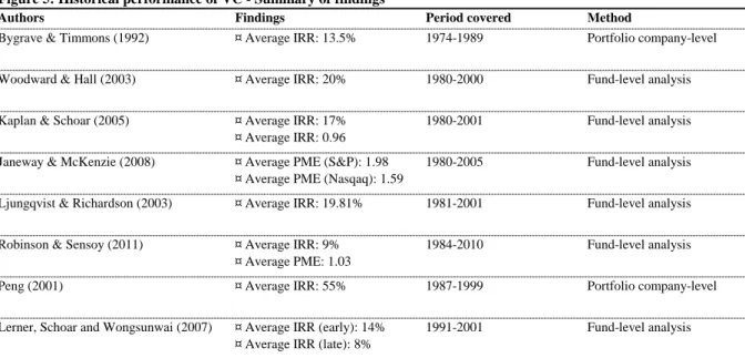
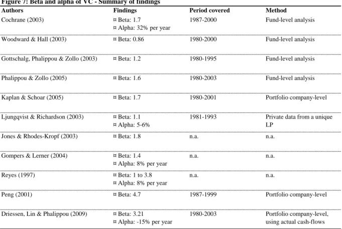
There is no consensus among academics regarding the performance of the venture capital industry, as we can see in the following table. All the PME numbers below, unless otherwise stated, are based on the performance of the S&P500.

As we can see, the results change significantly when compared to the performance of public markets. For example, Robinson and Sensoy report a pretty strong IRR of 9% over the 1984-2010 period, but a low PME of 1.03, meaning that funds have outperformed the S&P500 by only 3% over their life.

A second interesting point about public markets is the degree of systematic risk embedded in venture capital transactions. Previous research has extensively focused on this subject, and we have found necessary to describe the different methodologies used to estimate

Figure 5: Historical performance of VC - Summary of findings

Authors Findings Period covered Method

Bygrave & Timmons (1992) ¤ Average IRR: 13.5% 1974-1989 Portfolio company-level

Woodward & Hall (2003) ¤ Average IRR: 20% 1980-2000 Fund-level analysis

Kaplan & Schoar (2005) ¤ Average IRR: 17% ¤ Average IRR: 0.96

1980-2001 Fund-level analysis

Janeway & McKenzie (2008) ¤ Average PME (S&P): 1.98 ¤ Average PME (Nasqaq): 1.59

Ljungqvist & Richardson (2003) ¤ Average IRR: 19.81% 1981-2001 Fund-level analysis

Robinson & Sensoy (2011) ¤ Average IRR: 9% ¤ Average PME: 1.03

Peng (2001) ¤ Average IRR: 55% 1987-1999 Portfolio company-level

Lerner, Schoar and Wongsunwai (2007) ¤ Average IRR (early): 14% ¤ Average IRR (late): 8%

(16)

16 the beta of venture capital first, then to summarize the different estimates of alpha and beta of this asset class.

By definition, the beta measures the systematic risk of an asset compared to a benchmark, generally an index of publicly traded securities such as the S&P500. If represents the return of the S&P500 and the return of the observed fund, then the beta for this fund is

given by the following formula:

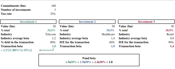
In order to estimate this beta, the first, straightforward approach has been used by Phalippou and Zollo (2005): for a given fund, they look at the quarterly reported IRR and the performance of the S&P500 during the same quarter. Then, they look at the covariance between the fund’s returns and the market return to get the beta and alpha coefficient in an OLS regression1. For their results to be valid, they rely on two strong assumptions: that the CAPM hold and that betas are the same within each industry. However, Kaplan and Schoar, using an investment-level approach, estimate the beta differently. For each investment made by the fund, they look at the average unlevered beta2 of the corresponding industry using traded comparable companies, then re-lever it using the capital structure used in the financing of the transaction. The method is explained in the figure below:

1

The principles of OLS regressions will be detailed in the next session of the paper.

2_{The unlevered beta does not take into account the capital structure of a project. If D denotes the amount of debt} used in the financing structure of the transaction, E the amount of equity and the tax rate, we have the following link between levered and unlevered betas: .

Figure 6: Estimation of the beta of VC - Kaplan and Schoar method

Commitments ($m) 100

Number of investments 3

Tax rate 35%

Investment 1 Investment 2 Investment 3

Value ($m) 20 Value ($m) 50 Value ($m) 30

% total 20,0% % total 50,0% % total 30,0%

Industry Telecom Industry Healthcare Industry Retail

Industry average beta 1,2 Industry average beta 1,4 Industry average beta 0,9

% debt in the transaction 80% D/E for the transaction 60% D/E for the transaction 90%

Transaction beta 1,8 Transaction beta 1,9 Transaction beta 1,4

= 1.2*[1+80%*(1-35%)]

Fund beta

(17)

17 Differently, to estimate whether venture capital funds bear some systematic risk exposure, Harris, Jenkinson and Kaplan (2013) tested the sensitivity of the PME measure to different beta levels. By successively assuming that VC investments earns respectively 1.0, 1.5 and 2.0 times the S&P500, they find really close PMEs, indicating a low correlation between the return of VC funds and the return of publicly traded securities. Cochrane (2005) and Gompers, Kovner, Lerner and Scharfstein (2005) find that the VC industry, far from being efficient1, is highly volatile compared to public markets, due to investors overreacting to perceived investment opportunities.

On the question of the level of systematic risk of venture capital funds, academics, to a certain extent, seem to reach a consensus, with a beta for this asset class slightly above 1, meaning that venture funds would slightly overreact to changes in public markets.

A last point of interest brought by previous research regarding the relationship between venture capital and public markets is the amount of capital flowing into the industry, influencing returns. The conclusion of many academics, including Ljungqvist and Richardson (2003), Lerner, Schoar and Wongsunwai (2007) and Robinson and Sensoy (2011) is that

1_{The “efficient market” hypothesis, developed by Eugene Fama, states that the price is always the right price} based on the fundamentals of the asset, and that consequently any change in the price should reflect a change in the fundamentals of the asset.

Figure 7: Beta and alpha of VC - Summary of findings

Authors Findings Period covered Method

Cochrane (2003) ¤ Beta: 1.7

¤ Alpha: 32% per year

Woodward & Hall (2003) ¤ Beta: 0.86 1980-2000 Fund-level analysis

Gottschalg, Phalippou & Zollo (2003) ¤ Beta: 1.2 1980-1995 Fund-level analysis

Phalippou & Zollo (2005) ¤ Beta: 1.6 1980-2003 Fund-level analysis

Kaplan & Schoar (2005) ¤ Beta: 1.7 1980-2001 Portfolio company-level

Ljungqvist & Richardson (2003) ¤ Beta: 1.1 ¤ Alpha: 5-6%

1981-1993 Private data from a unique LP

Jones & Rhodes-Kropf (2003) ¤ Beta: 1.8 n.a. n.a.

Gompers & Lerner (2004) ¤ Beta: 1.4

n.a. n.a.

Reyes (1997) ¤ Beta: 1 to 3.8

n.a. n.a.

Peng (2001) ¤ Beta: 4.7 1987-1999 Portfolio company-level

Driessen, Lin & Phalippou (2009) ¤ Beta: 3.21

¤ Alpha: -15% per year

1980-2003 Portfolio company-level,

(18)

18 venture capitalists tend to launch new funds in boom times, when public market valuations are high, but this strategy generally results in poor performance, suggesting for practitioners that a contrarian investment strategy would be successful if the historical pattern holds. For Kaplan and Schoar (2005), funds raised in times of high public markets valuations are less likely to raise follow-on funds, suggesting that they performed poorly. These deals, called “money chasing deals” by Gompers and Lerner (1999), are an important factor driving the overall performance of venture capital funds. Studying the link between public markets valuations, venture capital returns and the annual inflow into venture funds, they show that a year with high capital inflow is generally followed by a decrease in the average valuation for portfolio companies of VC funds. In line with the previously described papers of Cochrane (2005) and Gompers, Kovner, Lerner and Scharfstein (2005), they find that the venture capital market is not efficient. If finance theory teaches that the movements of equity prices, for publicly or privately owned companies, should be the consequence of a change either in the expected cash flows or in the firm’s cost of capital, they proved that inflows of money into the venture capital industry do influence the valuation of privately held companies and consequently the returns of the associated VC funds.

3.3 Individual performance drivers

It seems interesting to analyse the performance of funds and see whether we can find some individual characteristics that could help explain why top funds perform better than other funds, characteristics such as size, geography, stage-focus or speed of capital distribution.

There is a large consensus regarding the positive effect of size. Clearly, it appears that a fund size is positively correlated to its IRR or PME. Harris, Jenkinson and Kaplan (2013) show that, ranked by size, funds in the 3rd and 4th quartiles significantly underperform funds in the 2nd and 1st quartiles. The conclusion is the same for Kaplan and Schoar (2005) and Gottschalg, Phalippou and Zollo (2003), regardless of how performance is measured. Additionally, Kaplan and Schoar display a concave relationship between fund size and return, showing that top funds seem to limit their size even if they could raise more funds from outside investors. For Driessen, Lin and Phalippou (2009), larger funds perform better only because they have a higher risk exposure, not because they have higher alphas. This conclusion means that higher betas only drive the performance of big funds, and that these funds are not better managed or do not have any superior screening capability. Lerner, Schoar

(19)

19 and Wongsunwai (2007), on the contrary, taking the example of endowments, show how bigger funds perform better because of an early exposure to the venture capital industry and a better understanding of this asset class.

Some papers also point out geographical focus as a main individual driver of performance. The first consistent research by Hege, Palomino and Schwienbacher (2003) shows how contractual aspects differ between the United States, a mature venture capital market, and Europe, a relatively new market for venture financing, and are determinants in the success of a fund. But even more than geography, specialization is a main driver of return. As emphasized by Gompers, Kovner and Lerner (2009), generalist firms tend to underperform relative to specialist firms. This is explained by a better allocation across industries for specialist firms, as well as better investments due to a higher screening capability. However, these results can be mitigated when individuals among the generalist firm are industry specialists themselves.

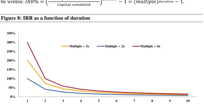
Speed of capital distribution is often cited as a driver of performance. Indeed, IRR can

be written: (

)

.

Figure 8: IRR as a function of duration

With a constant multiple, the IRR is decreasing in duration, as shown on the above figure. However, Hege, Palomino and Schwienbacher (2003) conclude that this theoretical relationship is only empirically verified in the US, where the longer the project, the lower the return. In Europe, the relation is reversed and venture capital funds benefit from longer investment. Their idea is that European funds, involved in a less mature market than their

0% 50% 100% 150% 200% 250% 300% 350% 1 2 3 4 5 6 7 8 9 10

(20)

20 American counterparts, learn about the quality of the project over time and thus a greater duration translates into an even higher multiple expansion.

3.4 Is there persistence in performance?

As for the previous section about the performance of VC funds compared to public markets, we would like here to focus first on the different methodologies used by academics, then on their conclusions.

First, we have to admit that little research has been performed on this subject for venture capital. Previous research has focused on other asset classes, for example mutual funds (see Kazemi, Schneeweis and Pancholi (2003) or Bollen and Buse (2005)) and has found no evidence of persistence. Robinson and Sensoy (2011) and Kaplan and Schoar (2005) use a common methodology based on a fund sequence number. The sequence number of a fund tells if the fund is the 1st, 2nd, 3rd etc. raised by the corresponding GP. Then, testing for the size effect and the persistence, they run the following regression, where e represents the error coefficient of the regression:

FundSize represents the logarithm of the capital committed to the fund and Sequence the logarithm of the sequence number1. In their paper, Janeway and McKenzie (2008) adopt a different approach, detailed and used by Kaplan and Schoar in a previous paper, to assess whether there is persistence in performance. Focusing on a sample of 205 fully liquidated funds over a 25-year long period, they regress the IRR of the latest fund of a GP with the IRR of the two previous funds launched by the same GP. The regression equation, where i is the sequence number of a fund, is as follow:

Both find that GPs whose fund outperformed are likely to raise successful follow-on funds in the future and vice-versa. This is due to the very specificity of the venture capital asset class. The observed persistence, say Janeway and McKenzie, “may well reflect the significant experience and contacts the LPs have accumulated after almost 30 years of investing”. Lerner, Schoar and Wongsunwai (2007) largely corroborate this view, saying that “anecdotes in the private equity industry suggest that established LPs often have preferential

1

(21)

21 access to funds”. These factors are also considered as crucial in the GP selection by LPs for Gomper, Kovner, Lerner and Scharfstein (2006) and Hochberg, Ljungqvist and Lu (2007).

3.5 Selection biases

In the literature, a recurring reservation is made about the potential biases that could exist in the sample selection. Two biases are generally pointed out in the papers: survivorship and selection. The first one, the survivorship bias, means that only existing funds can report the numbers we have access to. Funds which largely underperformed might be dead and might not report anymore. The second one, the selection bias, represents the opportunity for existing but low performing funds to stop reporting. Therefore, the reader should keep in mind that potentially much more failed transactions or negative IRRs exist beyond the ones reported in the database. The methodologies used largely differ, and we will focus only on the most recurring ones.

The first natural idea is, as explained by Ljungqvist and Richardson (2003), to work directly on a dataset sourced from a large LP that includes all the investments made without any bias, i.e. without withdrawing any low performing fund or investment from the sample. The problem is then to know how such an LP has performed compared to other LPs in order to make some general conclusions regarding the venture capital class as a whole.

Second, Kaplan and Schoar (2005) test a potential selective reporting which would result in an upward bias in the observed returns. They use a regression by constructing a dummy variable equal to 1 for the last quarter a fund reported an IRR and 0 otherwise to test whether or not GPs stopped reporting data after successive large negative returns. However, they find no evidence of funds stopping reporting after consecutive negative changes. Another concern they raise is that GPs could stop reporting as soon as they have either a particularly good performing fund (the GP managing the fund would like to “lock” the return) or a very bad performing one. Again, they find no evidence, as GPs of star funds are more likely to keep reporting, but this is more due to the higher probability of raising a follow-on fund afterwards.

Another convincing method used by Cochrane (2004), at an investment level, is the use of a model of the probability structure of the available data. His analysis relies upon a dataset of funds, between 1987 and 2000. To correct for the selection bias, he uses Heckman’s sample selection model. This model was originally built to address the problem of estimating the

(22)

22 average wage of women, using a dataset which excluded non-working women, i.e. housewives. The problem with private equity data is similar, as we are trying to estimate the average return using mainly data from successful funds, i.e. using data following a non-i.i.d. (independent and identically distributed) distribution. The problem is as follow: we are trying to find a relationship between IRR and, say, the size of the fund and its duration. However, this information is available only if the return reaches a certain acceptable threshold (say 10%). If is the vector (size, duration), we have the following problem:

Under the constraint: (1)

We observe: (2)

Heckman’s estimator is able to provide Cochrane with a value (for example, 15%), called Mills value. This value gives by how much the IRRs in his sample are shifted up due to the selection bias. The interpretation of this value is that the average IRR displayed in his sample is [ ] higher than a randomly selected IRR.

Using such a methodology, Cochrane finds a Mills coefficient of -1.97, and then concludes that the bias-corrected estimation reduces the average log return of venture capital funds from

108% to 15% and the alpha from 462% to 32%.

Figure 9: Peng and Cochrane's methodology

Step 1

Initial biased sample

Step 2

Get Mills value

Step 3

(23)

23

4 Research questions and hypotheses

In this section, we introduce the research questions that we aim to answer together with our expectations, based on the results synthetized in the literature review. As mentioned at the beginning of this paper, we would like to investigate three main topics regarding the performance of venture capital: the historical performance of VC funds and how it compares to public markets (1), the alpha and beta of this asset class (2) and whether individual characteristics of funds such as size, geography and stage specialization can help explain the performance of a fund (3).

Regarding the historical performance, we would like to understand the reason why investors are focusing more and more on venture capital in their asset allocation. Not only will we look at the absolute performance (IRR, MIRR), but we will also focus on the performance compared to public markets, using the public market equivalent (PME) measure.

Research question 1: What is the historical IRR yielded by venture capital funds over the 1983-2009 period?

Research question 2: Over this period, have VC funds outperformed or underperformed public markets?

Given the success of this asset class, we are expecting a high overall performance and a high PME as well. We expect to reach the conclusion by Robinson and Sensoy (2011) who cover the most recent period (1984-2010), that average IRR is around 9% per annum and the average PME is 1.03. Additionally, previous research has emphasized the dispersion in the performance of buyout funds, with top funds driving the whole performance of the industry (Phalippou and Zollo (2005)). We would like to see if this trend still holds for VC funds by analysing the dispersion of the different results.

The second research question is about the alpha and beta of VC. The beta is interesting as it translates the degree of correlation with the overall market.

Research question 3: What is the beta of venture capital?

Previous research to a certain extent agrees that the beta for VC funds is around 1.5. Our expectations are based on the most updated research paper, by Phalippou and Zollo (2005),

(24)

24 covering the 1980-2003 period, who found a beta of 1.6. It is more difficult to anticipate what alpha could be given the dispersion of previous findings.

Finally, we would like to identify to what extent individual characteristics of funds can be seen as drivers of performance. By investigating the relation between the performance and the size, geography, stage focus and duration, we would like to characterize the type of fund that outperforms and underperforms. Our fourth research question follows the findings of Harris, Jenkinson and Kaplan (2013) who show that, ranked by size, funds in the 3rd and 4th quartiles significantly underperform funds in the 2nd and 1st quartiles.

Research question 4: Is size positively correlated with a fund return?

The next interrogation is based on the paper of Hege, Palomino and Schwienbacher (2003), who find higher returns in the mature US market than in Europe.

Research question 5: Does the location of a fund significantly impact its return?

Then, we will study the performance by stage (early stage, later stage etc.). Little research exists on this subject, and our question is based on the findings of Lerner, Schoar and Wongsunwai (2007): early-stage funds significantly outperform later-stage funds.

Research question 6: Does performance vary according to the stage of specialisation?

Finally, we will check the theoretical relationship explained at the beginning of this paper, according to which duration tends to decrease the return of a fund, as shown on figure 8.

5 Dataset, variables and potential sample biases

5.1 Presentation of VentureXpert and potential sample biases

The VentureXpert database (previously called “Thomson Venture Economics” or “TVE”) is provided by Thomson Reuters and is considered the reference database, used in many previous research papers1. Contrary to some mutual fund databases (see Carhart, Carpenter and Lynch (2002)), VentureXpert does not drop data from the database if it falls below a certain IRR threshold. It is based exclusively on voluntary reporting by general and limited partners, which enables to crosscheck the information and improve the quality of the

1_{Google Scholar, as of March 20, 2014, identifies 332 academic papers using the query “VentureXpert” or} “Venture Economics” and “Performance”.

(25)

25 database. VentureXpert covers 3,844 funds (both venture and buyout funds) raised since 1969, and the data we have is updated through September 30, 2013 for US funds and June 30, 2013 for EMEA1 funds. For each fund, VentureXpert gathers individual information regarding its size, location, stage, vintage2 year, sequence number and whether the fund is liquidated or not. The returns displayed in the database are all net of management fees, carried interest and any potential partnership expense. Different performance measures are available:

 The traditionally used IRR, calculated using quarter-end valuations

 Distribution to paid-in capital (D/PI) measures the cash returned to investors (cash outflows) in proportion to the capital calls (cash inflows).

 Residual value to paid-in capital (RV/PI) measures how much of the cash given by LPs is still waiting to be invested.

 Total value to paid-in capital (TV/PI) is the sum of the two previous indicators and provides a rough estimate of the return to LPs for a non-liquidated fund. It is also called “money multiple” or “multiple” in the private equity industry.

 Paid-in to committed capital (PI/CC) gives the percentage of committed capital which has already been paid out to the GP by LPs.

 Distribution to committed capital (D/CC) is a measure of all the cash received by LPs in proportion to all the capital they committed into the fund.

From VentureXpert, we are able to get data using different filters: the vintage year, the fund stage and its location or size. Interestingly, VentureXpert displays aggregated performance metrics in different ways:

 The average and the median.

 The capital-weighted average and median, which take into account the relative size of each fund.

 Pooled returns: the pooled method treats all funds as a single fund by summing the monthly cash inflows and outflows altogether. It has the advantage to accounts for the scale and timing of cash flows.

However, given the privacy nature of the information and for computational reasons, VentureXpert makes some simplifying assumptions, as emphasized by Gottschalg, Phalippou and Zollo (2003). First, as soon as a cash flow is registered into the database, it is attributed to

1_{Europe, Middle East and Africa.} 2

(26)

26 the last day of the month in which it occurred. Second, distributions are often cash distributions, but they can also take the form of stocks. Stock distributions are recorded using the closing market price as of the distribution day. However, both LPs and GPs often have a lock-up period before being authorized to trade their shares, consequently this treatment of stock distributions is, to a certain extent, inaccurate. Moreover, the residual values, as previously defined, take into account cash, short-term and long-term equity investments, outstanding loans and other assets but exclude capital committed not drawn down.

The nature of the data and these simplifying assumptions result in sample biases. First, the data coming from voluntary reporting, the probability is strong to get a sample made of successful funds only. This is what we called “selection bias” and this is the bias overcome by Heckman’s estimator (remember: Heckman wanted to get the average salary of women, but could only gather data from employed women, excluding housewives who are part of the “women” population). This would create an upward bias in our sample. However, on the other side, VentureXpert might undervalue the return of non-liquidated funds given that residual values are valued at their accounting values. We mentioned in the literature review the findings of Gottschalg, Phalippou and Zollo (2003) who used a conversion matrix to account for residual value, after analysing how undervalued IRRs were for non-liquidated funds when using the accounting residual value. Similarly, for Stucke (2011), VentureXpert undervalues the return for non-liquidated funds. He provides evidence by comparing the correct ex-post fund performance (IRR and multiple of invested capital) with the estimate given by VentureXpert before liquidation for 140 funds. The graphs on the following page clearly show that “the vast majority of the data points are below / right of the diagonal line. These are funds for which TVE reports a lower performance than they achieved in reality”. The downward bias due to the use of accounting values as an estimate of residual values for non-liquidated funds is therefore evident.

To a certain extent, we can argue that the upward selection bias is partly offset by the downward bias coming from accounting values for non-liquidated funds and that the returns provided by VentureXpert should be good estimates of the “true” return of venture capital.

(27)

27 Figure 10: Strucke (2011) – Comparison of the TVE sample with correct performance data

This figure compares the IRRs (Chart A) and multiples of invested capital (Chart B) of incomplete U.S. funds from the TVE sample with correct performance data from LPs. The abscissa contains the (correct) values of the LP data. The ordinate contains the corresponding values presented by TVE. The scale of the axes is limited to -20% and +40% (Chart A), and to money multiples of up to 3.0 (Chart B).

5.2 Dataset and variables

This section first describes the dataset and provides some interesting descriptive statistics about our sample of funds. Then, we describe the way we collect the data and build the variables which will be used to measure the performance in the last part of this paper.

(28)

28 VentureXpert gathers data for 2,166 venture capital funds. We have applied a number of filters to retain only the most relevant ones. First, very little data is available for funds raised before 1983 and consequently it would not have been statistically relevant to include such funds. Our sample is therefore made of funds whose vintage year is 1983 or later. Additionally, we have chosen not retain funds raised after 2009, given that the committed capital might not have been invested yet and the numbers, as shown by Strucke, would have been too biased. This results in a sample with the majority of the committed capital being invested already, limiting the potential biases in our results.

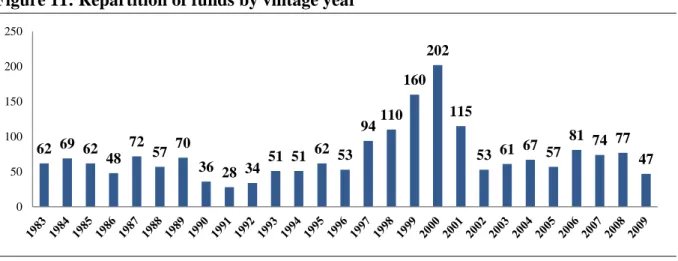
Finally, our dataset consists of 1,953 funds launched over the period of 1983-2009 (27 years), the largest period ever covered by previous research (Robinson and Sensoy covered 26 years). Figure 11 below displays the repartition of funds by vintage year.

Figure 11: Repartition of funds by vintage year

As the coverage of the VentureXpert database is the best among all the available databases, we can assume that this sample is representative of the whole VC industry. A first observation is that this graph clearly shows the different cycles in the industry, with a first wave of funds raised between 1983 and 1989, a second wave between 1997 and 2001, corresponding the Internet bubble and a last one in the years 2006, 2007 and 2008 when the private equity industry activity reached a peak.

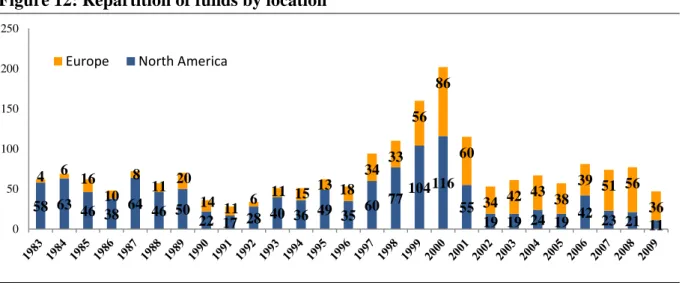
Figure 12 shows the geographical split of our sample. For the analysis by location, we have retained all the 1,953 funds split between “North America” (Canada and the US) and “Europe” (Western Europe, France, Germany and the UK mainly). As emphasized by Hege, Palomino and Schwienbacher (2003), this graph reveals that the American VC market is much mature, as the 1983 level (58 funds raised this year) in the US has been reached in 1999

62 69 62 48 72 57 70 36 28 34 51 51 62 53 94 110 160 202 115 53 61 67 57 81 74 77 47 0 50 100 150 200 250

(29)

29 in Europe (56 funds raised). If the European VC industry has emerged later than in the US, they both follow the same previously described cycles.

Figure 12: Repartition of funds by location

Below is the repartition of funds by vintage year and by size. The different size ranges provided by VentureXpert are the following: [$0m;$30m], [$30m;$50m], [$50m;$100m], [$100m;$300m], [$300m;$500m], [$500m;$1000m] and [$1000m;$1000m+]. For our analysis, we have retained all the intervals, even if some of them contain little data. We can notice that size repartition does not seem to have changed during the time period we have selected, except for big funds above $300m, which seem to represent a higher percentage of total funds during peak periods and vice-versa.

Figure 13: Repartition of funds by size bracket

VC funds are in majority small-size funds below 100m but size increases when higher returns are perceived, i.e. during bubbles (1983-1990, 1997-2001 and 2006-2008). A first hypothesis

58 63 46 38 64 46 50 22 17 28 40 36 49 35 60 77 104 116 55 19 19 24 19 42 _{23 21 11} 4 6 16 10 8 11 20 14 11 6 11 15 13 18 34 33 56 86 60 34 42 43 38 39 51 56 36 0 50 100 150 200 250

Europe North America

0 20 40 60 80 100 120 140 160 180

200 _{1000.1 Mil+} _{500.1 - 1000 Mil} _{300.1 - 500 Mil}

100.1 - 300 Mil 50.1 - 100 Mil 30.1 - 50 Mil 0 - 30 Mil

(30)

30 could be that institutional investors allocate a higher part of their portfolio to venture capital when the overall sentiment is positive.

Figure 14: Repartition of funds by stage focus

The different stages have previously been described in this paper. “Balanced” represents non-specialized funds that can invest in either seed, early or later-stage companies. From this graph, we see that VC funds are primarily focused on early-stage companies or not focused on any type, i.e., balanced. The split between early-stage, later-stage and balanced funds seems to hold during all the period. The pattern only changes between 1997 and 2001, the dotcom bubble, when funds were mainly early-stage funds investing massively in Internet start-ups.

We will now describe the different measures used in our analysis and the way we build them. As described above, our sample is made of funds raised between 1983 and 2009.

1st part: Historical performance of VC funds and comparision with public markets

The first part of our analysis is dedicated to the historical performance of VC funds by vintage year. We focus on 4 previously introduced measures: the IRR, the modified IRR (MIRR), the public market equivalent (PME) and the TV/PI (“Total value / Paid-in capital”) multiple. We collected these measures in two different ways:

 A first file gives, for each fund, its vintage year, stage, location, size range, IRR and TV/PI multiple. For funds still active, VentureXpert estimates the residual value of cash-flows and we then have data for funds raised between 1983 and 2009.

 A second file provides aggregated cash-flow data by vintage year. For every quarter from January 1983 to September 2013, we know how much money funds raised in 1983, 1984,…, 2009 distributed and took down from investors. From this, we then

0 50 100 150 200 250

Seed Stage Later Stage

(31)

31 9th decile 3rd quartile Median 1st quartile 1st decile

calculate two MIRRs, using reinvestment rates of 8% (the “hurdle rate”) and 10% and two IRRs, one using the S&P500 as benchmark and the other one using the Nasdaq Composite Index. However, this cash-flow based methodology only enables us to use data for funds raised between 1983 and 2003. Funds raised after 2004 are still active and therefore we lack a significant part of the distributions, which would average our results downward.

It is interesting for us to use these two methods, one using data aggregated by VentureXpert for each vintage year and the other one using the actual cash-flows. We will be able to cross-check our results.

From the first file, we build box plots for each vintage year using the IRR to understand how performance varied in time. The box plot follows the following scheme:

the 1st and 9th deciles show the outliers, i.e. the top 10% and the worst 10% funds ranked by IRR. The 1st quartile (3rd) splits off the lowest 25% of data (75%). The distance between the 1st and the 3rd quartile, called the interquartile range, represents the dispersion of the performance of the funds raised during this given vintage year. Finally, the median is the number where half funds have a higher performance and the other half have lower IRRs.

From the second file, we build MIRRs and PMEs to compare the performance with public markets. For each vintage year, we use the previously described methodology to calculate MIRRs and PMEs: for the MIRR calculation, we discount all the drawdowns using 8% and compound all the distributions using the same rate. However, as we are using aggregated data for funds raised during the same vintage year, it often happens that a few funds are still not liquidated after 15 years or more and continue to distribute cash-flows back to investors. In order not to skew our results, we consider that the last cash-flow occurs when 98% of all the distributions from funds raised in a same vintage year have been given back to investors. We then reiterate this operation using a 10% reinvestment rate for the second M-IRR calculation. The goal is to understand how sensitive our results are to the chosen rate and check that the return patterns we find are not dependent on the rate used in the MIRR calculation.

The PME calculation is based on the same cash-flow schedule displayed by the database for each vintage year. It is calculated following the previous example, i.e. discounting all the cash

(32)

32 inflows and outflows with the market return. Again, to crosscheck our results, we have found interesting to calculate the PME based on the S&P500 quarterly returns and the NASDAQ returns as well. By definition, the S&P500 is a market-value weighted index, i.e. each stock weights its relative market capitalization, based on 500 leading companies in diversified industries. It is considered to be a good benchmark for the overall US stock market and, more generally, the world market. The comparison with the NASDAQ seems interesting to us as the NASDAQ is a market-capitalization weighted index made of more than 3,000 stocks listed on the Nasdaq stock exchange. The companies covered by this index are mainly Internet-related companies, which is interesting in the context of venture capital. In order to check the consistence of our results, we will also use traditional statistical t-tests.

2nd part: the alpha and beta of venture capital

The second part of our research is dedicated to the alpha and beta of venture capital. We will use Phalippou and Zollo (2005) method and look at the covariance between VC funds’ returns and the market return to get the beta and alpha coefficient in an OLS regression1. This method assumes that the two following conditions hold:

 CAPM holds

 Betas are the same in each industry

We cannot use the two previously described files, as the results are given for each vintage year, and we need here to construct a venture capital index. We will use the “PE Index” from VentureXpert. The Private Equity Index reflects the aggregated returns of private equity funds and is calculated based on the quarterly percent change of the net appreciation of net asset values, as previously defined, taking into account cash-flows during the period, starting with a base 100 in January 1983. We will run the regression using quarterly available data, the most granular data available. We believe this is more relevant than annual data, as a lot of information is present when using returns over short intervals. Moreover, given the

1_{By definition, according to the CAPM, the return of any asset follows this equation:}

[ ] . We will get such a relationship between the return of VC funds and public markets for every quarter. The OLS regression will provide us with alpha and beta coefficient estimates such as: