Supplemental Information 1 Habitat loss on the breeding grounds is a major contributor to population declines in a 2 long-distance migratory songbird 3 Michael T. Hallworth

(1)

Supplemental Information

1 Habitat loss on the breeding grounds is a major contributor to population declines in a

2 long-distance migratory songbird

3 Michael T. Hallworth

1

_{*, Erin Bayne}

2

_{, Emily McKinnon}

3

_{, Oliver Love}

3

_{, Junior A. Tremblay}

4

_,

4 Bruno Drolet

4

_{, Jacques Ibarzabal}

5

_{, Steven Van Wilgenburg}

6

_{, and Peter P. Marra}

1

5

1

_{Migratory Bird Center, Smithsonian Conservation Biology Institute. Washington, D.C. 20008,}

6 U.S.A.

7

2

_{University of Alberta, Alberta, Canada}

8

3

_{University of Windsor, Ontario, Canada}

9

4

_{Environment and Climate Change Canada, Québec, Canada}

10

5

_{Université du Québec á Chicoutimi, Saguenay, Canada}

11

6

_{Environment and Climate Change Canada, Saskatchewan, Canada}

12 ’* Corresponding Author:

mhallworth@gmail.com

13

(2)

Supplemental Methods

15 Light-level geolocation

16 We defined twilight (sunrise and sunset events) using the

findTwilights

function with a

17 threshold of 1. Sunrise and sunset times were assigned as the time the ambient light-levels

18 recorded by the geolocator rose above and fell below the threshold value, respectively. We set a

19 minimum dark period of six hours to remove spurious twilight events. Once twilights were

20 determined with used the changeLight function available in the GeoLight package [1] to identify

21 migratory phenology using a stationary duration of two days. We subsequently merged

22 stationary locations that were closer than 300 km. We used informative behavioral priors in our

23 analysis to help refine location estimates. We used two distinct flight speed models within our

24 behavioral model, one corresponding to stationary periods and another to migratory periods ([2],

25 Fig. S2

). In addition to using different flight speed parameters we used different zenith angles

26 throughout the year [3,4]. We determined the zenith angle associated with each identified

27 stationary period using the findHEzenith function available in the GeoLight package [1].

28 Geographic coordinates estimated while including uncertainty inherent in light-level geolocation

29 [5] were derived by combining a model describing the difference between observed and expected

30 twilight times, a behavioral movement model and a land mask which restricted stationary periods

31 of the annual cycle to land masses while allowing flights to occur over water [6,7]. We ran the

32 MCMC analysis using a Metropolis sampler. We made our geographic inference from 5000

33 draws from the posterior distribution following an initial burn-in phase of 1000 draws.

34 Habitat loss & fragmentation

35

(3)

Habitat loss was summarized from the Global Forest Change data set (version 1.6; [8]) using

36 Google Earth Engine [9]. We summarized the area of habitat loss in each year between 2000 and

37 2017 within each 500km x 500km target location (see Migratory Connectivity) and calculated

38 the cumulative loss across years. For each population we derived a weighted average of habitat

39 loss that accounts for location uncertainty. We used the estimated probability that a population

40 used a particular 500km x 500km region derived from the MC metric to calculate a weighted

41 average

Fig. S1

). We present the annual rate of change as a summary statistic because the area of

42 inference differed between breeding (∼ 7850 km^2) and non-breeding seasons (250,000 km^2).

43 Within our analysis we used the cumulative habitat loss. In addition to habitat loss, we derived

44 several metrics that describe habitat fragmentation within each landscape. We calculated the

45 percentage of forest cover (PLAND), edge density (ED), patch density (PD), nearest patch (NP),

46 largest patch index (LPI), total core area (TCA), and core area index (CAI) metrics [10] using the

47 LandscapeMetrics R package [11]. Several of the metrics were highly correlated (r > 0.75, Fig.

48 S3) and were removed from the analysis to reduce redundancy. We included the largest patch

49 index (LPI) which is an area to edge metric that approaches 0 when the largest patch becomes

50 small and approaches 100 when the landscape is comprised of a single patch, number of patches

51 (NP) which is an aggregation metric that describes the number of patches within the landscape

52 but does not contain information about how patches are configured within the landscape. Finally,

53 we included total core area (TCA) which is a configuration metric that describes the amount of

54 core area (non-edge habitat) within a landscape [11]. For each metric we used 8 neighbors

55 (queen’s case) and did not consider pixels at the edge of the landscape boundary as core area. For

56 fragmentation metrics that calculated edge we used 90m or 3 raster cells (30m x 30m resolution)

57 as the distance from edge to be considered core.

58

(4)

Supplemental Results

59 Habitat loss & fragmentation

60 The amount of core forested habitat (total core area) declined at the greatest rate at stopover

61 regions prior to making longdistance over water flights (mean = 124.71, range = 228.29

-62

65.49 thousand ha

-yr

_{) followed by the stationary non-breeding landscapes (mean = -28.45, range}

63 = -38.98 - -2.57 thousand ha

-yr

_{), stopover regions post Atlantic crossing (mean = -49.79, range =}

64 -79.41 - -15.13 thousand ha

-yr

_{) and finally the breeding grounds (mean = -14.01, range = -21.57}

65 - -7.29 thousand ha

-yr

_).

66

(5)

Supplemental Tables

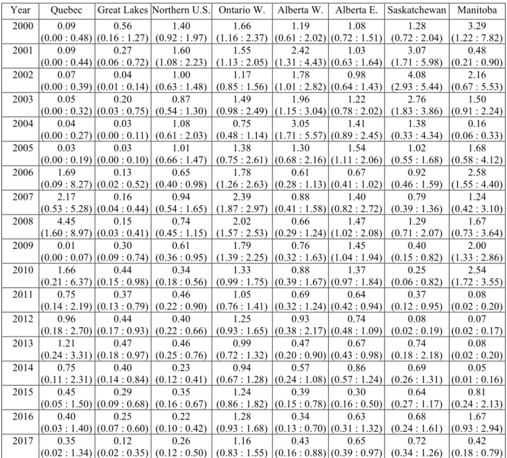
68 Table S1. Mean abundance and 95% credible interval of Connecticut warblers along breeding

69 bird survey routes within each of the ‘natural’ populations.

70

Year Quebec Great Lakes Northern U.S. Ontario W. Alberta W. Alberta E. Saskatchewan Manitoba

2000 0.09 (0.00 : 0.48) (0.16 : 1.27) 0.56 (0.92 : 1.97) 1.40 (1.16 : 2.37) 1.66 (0.61 : 2.02) 1.19 (0.72 : 1.51) 1.08 (0.72 : 2.04) 1.28 (1.22 : 7.82) 3.29 2001 0.09 (0.00 : 0.44) (0.06 : 0.72) 0.27 (1.08 : 2.23) 1.60 (1.13 : 2.05) 1.55 (1.31 : 4.43) 2.42 (0.63 : 1.64) 1.03 (1.71 : 5.98) 3.07 (0.21 : 0.90) 0.48 2002 0.07 (0.00 : 0.39) 0.04 (0.01 : 0.14) 1.00 (0.63 : 1.48) 1.17 (0.85 : 1.56) 1.78 (1.01 : 2.82) 0.98 (0.64 : 1.43) 4.08 (2.93 : 5.44) 2.16 (0.67 : 5.53) 2003 0.05 (0.00 : 0.32) (0.03 : 0.75) 0.20 (0.54 : 1.30) 0.87 (0.98 : 2.49) 1.49 (1.15 : 3.04) 1.96 (0.78 : 2.02) 1.22 (1.83 : 3.86) 2.76 (0.91 : 2.24) 1.50 2004 0.04 (0.00 : 0.27) (0.00 : 0.11) 0.03 (0.61 : 2.03) 1.08 (0.48 : 1.14) 0.75 (1.71 : 5.57) 3.05 (0.89 : 2.45) 1.41 (0.33 : 4.34) 1.38 (0.06 : 0.33) 0.16 2005 0.03 (0.00 : 0.19) (0.00 : 0.10) 0.03 (0.66 : 1.47) 1.01 (0.75 : 2.61) 1.38 (0.68 : 2.16) 1.30 (1.11 : 2.06) 1.54 (0.55 : 1.68) 1.02 (0.58 : 4.12) 1.68 2006 1.69 (0.09 : 8.27) 0.13 (0.02 : 0.52) 0.65 (0.40 : 0.98) 1.78 (1.26 : 2.63) 0.61 (0.28 : 1.13) 0.67 (0.41 : 1.02) 0.92 (0.46 : 1.59) 2.58 (1.55 : 4.40) 2007 2.17 (0.53 : 5.28) (0.04 : 0.44) 0.16 (0.54 : 1.65) 0.94 (1.87 : 2.97) 2.39 (0.41 : 1.58) 0.88 (0.82 : 2.72) 1.40 (0.39 : 1.36) 0.79 (0.42 : 3.10) 1.24 2008 4.45 (1.60 : 8.97) (0.03 : 0.41) 0.15 (0.45 : 1.15) 0.74 (1.57 : 2.53) 2.02 (0.29 : 1.24) 0.66 (1.02 : 2.08) 1.47 (0.71 : 2.07) 1.29 (0.73 : 3.64) 1.67 2009 0.01 (0.00 : 0.07) (0.09 : 0.74) 0.30 (0.36 : 0.95) 0.61 (1.39 : 2.25) 1.79 (0.32 : 1.63) 0.76 (1.04 : 1.94) 1.45 (0.15 : 0.82) 0.40 (1.33 : 2.86) 2.00 2010 1.66 (0.21 : 6.37) 0.44 (0.15 : 0.98) 0.34 (0.18 : 0.56) 1.33 (0.99 : 1.75) 0.88 (0.39 : 1.67) 1.37 (0.97 : 1.84) 0.25 (0.06 : 0.82) 2.54 (1.72 : 3.55) 2011 0.75 (0.14 : 2.19) (0.13 : 0.79) 0.37 (0.22 : 0.90) 0.46 (0.76 : 1.41) 1.05 (0.32 : 1.24) 0.69 (0.42 : 0.94) 0.64 (0.12 : 0.95) 0.37 (0.02 : 0.20) 0.08 2012 0.96 (0.18 : 2.70) (0.17 : 0.93) 0.44 (0.22 : 0.66) 0.40 (0.93 : 1.65) 1.25 (0.38 : 2.17) 0.93 (0.48 : 1.09) 0.74 (0.02 : 0.19) 0.08 (0.02 : 0.17) 0.07 2013 1.21 (0.24 : 3.31) 0.47 (0.18 : 0.97) 0.46 (0.25 : 0.76) 0.99 (0.72 : 1.32) 0.47 (0.20 : 0.90) 0.67 (0.43 : 0.98) 0.74 (0.18 : 2.18) 0.08 (0.02 : 0.20) 2014 0.75 (0.11 : 2.31) (0.14 : 0.84) 0.40 (0.12 : 0.41) 0.23 (0.67 : 1.28) 0.94 (0.24 : 1.08) 0.57 (0.57 : 1.24) 0.86 (0.26 : 1.31) 0.69 (0.01 : 0.16) 0.05 2015 0.45 (0.05 : 1.50) (0.09 : 0.68) 0.29 (0.16 : 0.67) 0.35 (0.86 : 1.82) 1.24 (0.15 : 0.78) 0.39 (0.16 : 0.50) 0.30 (0.27 : 1.17) 0.64 (0.24 : 2.13) 0.81 2016 0.40 (0.03 : 1.40) (0.07 : 0.60) 0.25 (0.10 : 0.42) 0.22 (0.93 : 1.68) 1.28 (0.13 : 0.70) 0.34 (0.31 : 1.32) 0.63 (0.24 : 1.61) 0.68 (0.93 : 2.94) 1.67 2017 0.35 (0.02 : 1.34) 0.12 (0.02 : 0.35) 0.26 (0.12 : 0.50) 1.16 (0.83 : 1.55) 0.43 (0.16 : 0.88) 0.65 (0.39 : 0.97) 0.72 (0.34 : 1.26) 0.42 (0.18 : 0.79)

71

72

(6)

Supplemental Figures

73 Fig. S1 The target regions (500km x 500km) used to estimate the strength of migratory

74 connectivity (MC) for Connecticut warblers between breeding and significant stopover locations

75 (A. pre Atlantic crossing, B. post Atlantic crossing) and the stationary non-breeding season (C).

76 The target regions outlined in black were the regions with a transition probability greater than 0

77 identified in the migratory connectivity analysis. The target regions outlined in white were

78 included as possible target regions but were not used by populations in our analysis. The lines

79 connect the breeding location with the target regions used by a population. The width of the line

80 represents that transition probability from the breeding site to the target regions - wide lines

81 represent a greater probability a given population used that target region. Figure S1 D shows an

82 enlarged region in South America where Connecticut warblers spent the stationary non-breeding

83 season.

84 Fig. S2 The flight behavior mask used for stationary (solid line) and migratory (dotted) phases of

85 the annual cycle. We allowed for a greater flight speed during migratory periods than during

86 stationary periods.

87 Fig. S3 A scatterplot matrix showing the correlation and correlation coefficients between

88 landscape fragmentation metrics. For each landscape we derived the percentage of forest cover

89 (PLAND), edge density (ED), patch density (PD), nearest patch (NP), largest patch index (LPI),

90 total core area (TCA), and core area index (CAI_mn) using the LandscapeMetrics package [11].

91 Fig. S4 Posterior predictive diagnostic of model fit for habitat loss (A) and habitat fragmentation

92 (B) using Chi-square goodness of fit test statistic.

93

(7)

Fig. S5 Connecticut warbler observation locations submitted to eBird.org by community

94 scientists (also referred to as citizen scientists). Observations are color coded by season and size

95 of the locations is representative of the number of individuals seen at that location. While spring

96 migration routes of individuals are unknown, eBird checklists suggest that the geographic

97 regions used by Connecticut warblers during spring and fall migration are similar.

98

(8)

Fig. S1

100

101

102

(9)

Fig. S2

103

104

105

(10)

Fig. S3

106

107

108

(11)

Fig. S4

109

110

111

(12)

Fig. S5

112

113

114

(13)

Supplemental References

115 1. Lisovski S, Hewson CM, Klaassen RHG, Korner-Nievergelt F, Kristensen MW, Hahn S.

116 2012 Geolocation by light: accuracy and precision affected by environmental factors.

117 Methods in Ecology and Evolution

118 2. Schmaljohann H, Lisovski S, Bairlein F. 2017 Flexible reaction norms to environmental

119 variables along the migration route and the significance of stopover duration for total speed

120 of migration in a songbird migrant. Frontiers in Zoology 14, 17.

(doi:10.1186/s12983-017-121

0203-3)

122 3. Hallworth MT, Sillett TS, Van Wilgenburg SL, Hobson KA, Marra PP. 2015 Migratory

123 connectivity of a Neotropical migratory songbird revealed by archival light-level

124 geolocators. Ecological Applications 25, 336–347. (doi:10.1890/14-0195.1)

125 4. McKinnon EA, Stanley CQ, Fraser KC, MacPherson MM, Casbourn G, Marra PP, Studds

126 CE, Diggs N, Stutchbury BJ. 2013 Estimating geolocator accuracy for a migratory songbird

127 using live ground-truthing in tropical forest. Animal Migration 1, 31–38.

128 5. Lisovski S et al. 2018 Inherent limits of light-level geolocation may lead to

over-129

interpretation. Current Biology 28, R99–R100. (doi:10.1016/j.cub.2017.11.072)

130 6. Lisovski S et al. 2020 Light-level geolocator analyses: A user’s guide. Journal of Animal

131 Ecology 89, 221–236. (doi:10.1111/1365-2656.13036)

132 7. Cooper NW, Hallworth MT, Marra PP. 2017 Light-level geolocation reveals wintering

133 distribution, migration routes, and primary stopover locations of an endangered long-distance

134 migratory songbird. J Avian Biol 48, 209–219. (doi:10.1111/jav.01096)

135 8. Hansen MC et al. 2013 High-Resolution Global Maps of 21st-Century Forest Cover Change.

136 Science 342, 850–853. (doi:10.1126/science.1244693)

137 9. Gorelick N, Hancher M, Dixon M, Ilyushchenko S, Thau D, Moore R. 2017 Google Earth

138 Engine: Planetary-scale geospatial analysis for everyone. Remote Sensing of Environment

139 202, 18–27. (doi:10.1016/j.rse.2017.06.031)

140 10. Wang X, Blanchet FG, Koper N. 2014 Measuring habitat fragmentation: An evaluation of

141 landscape pattern metrics. Methods in Ecology and Evolution 5, 634–646.

142 (doi:10.1111/2041-210X.12198)

143 11. Hesselbarth MHK, Sciaini M, With KA, Wiegand K, Nowosad J. 2019 landscapemetrics: an

144 open-source R tool to calculate landscape metrics. Ecography 42, 1648–1657.

145 (doi:10.1111/ecog.04617)

146

147

148

(14)

Appendix 1. JAGS model

149

## model{

150

## # THIS IS A POISSON REGRESSION TO ESTIMATE CONNECTICUT WARBLER ABUNDANCE

151

## # USING BBS ROUTE LEVEL TOTALS FOLLOWING RUSHING ET AL. 2016 JAE

152

##

153

## # model indicator variable as joint distribution to facilitate mixing

154

## # Hooten & Hobbs 2015, AHM vol 1. Kery & Royle pg 342

155

##

156

## # Priors

157

## HyperTrend ~ dnorm(0,0.01)

158

## HyperAlpha ~ dnorm(0,0.01)

159

## # forest loss hyper priors #

160

## Hyper_cumbreed ~ dnorm(0,0.01)

161

## Hyper_cumwinter ~ dnorm(0,0.01)

162

## Hyper_cumpre ~ dnorm(0,0.01)

163

## Hyper_cumpost ~ dnorm(0,0.01)

164

## Hyper_cumloss ~ dnorm(0,0.01)

165

## # fragmentation priors

166

## Hyper_lpi ~ dnorm(0,0.01)

167

## Hyper_np ~ dnorm(0,0.01)

168

## Hyper_tca ~ dnorm(0,0.01)

169

## Hyper_npwinter ~ dnorm(0,0.01)

170

## Hyper_nppre ~ dnorm(0,0.01)

171

## Hyper_nppost ~ dnorm(0,0.01)

172

## Hyper_lpiwinter ~ dnorm(0,0.01)

173

## Hyper_lpipre ~ dnorm(0,0.01)

174

## Hyper_lpipost ~ dnorm(0,0.01)

175

## Hyper_tcawinter ~ dnorm(0,0.01)

176

## Hyper_tcapre ~ dnorm(0,0.01)

177

## Hyper_tcapost ~ dnorm(0,0.01)

178

## Hyper_obs ~ dnorm(0,0.01)

179

## Hyper_eps ~ dnorm(0,0.001)

180

##

181

## # Priors for population-level intercept

182

## # and indicator variable for cumulative breeding

183

## # forest loss

184

##

185

## for(p in 1:npopulations){

186

## # intercept

187

## alpha[p] ~ dnorm(HyperAlpha,tau.alpha)

188

## beta.trend[p] ~ dnorm(HyperTrend,tau.trend)

189

##

190

## # prior indicators #

191

(15)

## pop.breed.ind[p] ~ dbeta(5,5)

192

## pop.lpi.ind[p] ~ dbeta(5,5)

193

## pop.np.ind[p] ~ dbeta(5,5)

194

## pop.tca.ind[p] ~ dbeta(5,5)

195

##

196

## # realized indicators #

197

## breed.ind[p] ~ dbern(pop.breed.ind[p])

198

## breed.lpi.ind[p] ~ dbern(pop.lpi.ind[p])

199

## breed.np.ind[p] ~ dbern(pop.np.ind[p])

200

## breed.tca.ind[p] ~ dbern(pop.tca.ind[p])

201

##

202

## # joint beta & indicator #

203

## beta_cumbreed[p] ~ dnorm(Hyper_cumbreed, tau.cumBreed)

204

## beta.cumbreed[p] <- breed.ind[p]*beta_cumbreed[p]

205

##

206

## beta_breed_lpi[p] ~ dnorm(Hyper_lpi, tau.breedLPI)

207

## beta.breed.lpi[p] <- breed.lpi.ind[p]*beta_breed_lpi[p]

208

##

209

## beta_breed_np[p] ~ dnorm(Hyper_np, tau.breedNP)

210

## beta.breed.np[p] <- breed.np.ind[p]*beta_breed_np[p]

211

##

212

## beta_breed_tca[p] ~ dnorm(Hyper_tca, tau.breedTCA)

213

## beta.breed.tca[p] <- breed.tca.ind[p]*beta_breed_tca[p]

214

## }

215

##

216

## # HARD CODE BETA ESTIMATES FOR WINTER, PRE AND POST FLIGHT LOSS TO 0

217

## # FOR POPULATIONS WHERE WE DON'T HAVE TRACKING INFORMATION FOR

218

## # we have info from 1,3,4,6

219

## for(tp in c(1,3,4,6)){ # tp = tracked population

220

## # Cumulative loss during winter

221

## pop.winter.ind[tp] ~ dbeta(5,5)

222

## winter.ind[tp] ~ dbern(pop.winter.ind[tp])

223

## beta_cumwinter[tp] ~ dnorm(Hyper_cumwinter, tau.cumWinter)

224

## beta.cumwinter[tp] <- winter.ind[tp]*beta_cumwinter[tp]

225

##

226

## # Cumulative loss pre flight

227

## pop.pre.ind[tp] ~ dbeta(5,5)

228

## pre.ind[tp] ~ dbern(pop.pre.ind[tp])

229

## beta_cumpre[tp] ~ dnorm(Hyper_cumpre, tau.cumPre)

230

## beta.cumpre[tp] <- pre.ind[tp]*beta_cumpre[tp]

231

##

232

## # Cumulative loss post flight

233

## pop.post.ind[tp] ~ dbeta(5,5)

234

## post.ind[tp] ~ dbern(pop.post.ind[tp])

235

## beta_cumpost[tp] ~ dnorm(Hyper_cumpost, tau.cumPost)

236

(16)

## beta.cumpost[tp] <- post.ind[tp]*beta_cumpost[tp]

237

##

238

## # Cumulative loss post flight

239

## pop.cumloss.ind[tp] ~ dbeta(5,5)

240

## cumloss.ind[tp] ~ dbern(pop.cumloss.ind[tp])

241

## beta_cumloss[tp] ~ dnorm(Hyper_cumloss, tau.cumLoss)

242

## beta.cumloss[tp] <- cumloss.ind[tp]*beta_cumloss[tp]

243

##

244

## # lpi

245

## # winter

246

## lpi.winter.ind[tp] ~ dbeta(5,5)

247

## winter.lpi.ind[tp] ~ dbern(lpi.winter.ind[tp])

248

## beta_winter_lpi[tp] ~ dnorm(Hyper_lpiwinter, tau.lpiWinter)

249

## beta.winter.lpi[tp] <- winter.lpi.ind[tp]*beta_winter_lpi[tp]

250

## # pre

251

## lpi.pre.ind[tp] ~ dbeta(5,5)

252

## pre.lpi.ind[tp] ~ dbern(lpi.pre.ind[tp])

253

## beta_pre_lpi[tp] ~ dnorm(Hyper_lpipre, tau.lpiPre)

254

## beta.pre.lpi[tp] <- pre.lpi.ind[tp]*beta_pre_lpi[tp]

255

## # post

256

## lpi.post.ind[tp] ~ dbeta(5,5)

257

## post.lpi.ind[tp] ~ dbern(lpi.post.ind[tp])

258

## beta_post_lpi[tp] ~ dnorm(Hyper_lpipost, tau.lpiPost)

259

## beta.post.lpi[tp] <- post.lpi.ind[tp]*beta_post_lpi[tp]

260

##

261

## # tca

262

## # winter

263

## tca.winter.ind[tp] ~ dbeta(5,5)

264

## winter.tca.ind[tp] ~ dbern(tca.winter.ind[tp])

265

## beta_winter_tca[tp] ~ dnorm(Hyper_tcawinter, tau.tcaWinter)

266

## beta.winter.tca[tp] <- winter.tca.ind[tp]*beta_winter_tca[tp]

267

## # pre

268

## tca.pre.ind[tp] ~ dbeta(5,5)

269

## pre.tca.ind[tp] ~ dbern(tca.pre.ind[tp])

270

## beta_pre_tca[tp] ~ dnorm(Hyper_tcapre, tau.tcaPre)

271

## beta.pre.tca[tp] <- pre.tca.ind[tp]*beta_pre_tca[tp]

272

## # post

273

## tca.post.ind[tp] ~ dbeta(5,5)

274

## post.tca.ind[tp] ~ dbern(tca.post.ind[tp])

275

## beta_post_tca[tp] ~ dnorm(Hyper_tcapost, tau.tcaPost)

276

## beta.post.tca[tp] <- post.tca.ind[tp]*beta_post_tca[tp]

277

##

278

## # np

279

## # winter

280

## np.winter.ind[tp] ~ dbeta(5,5)

281

(17)

## winter.np.ind[tp] ~ dbern(np.winter.ind[tp])

282

## beta_winter_np[tp] ~ dnorm(Hyper_npwinter, tau.npWinter)

283

## beta.winter.np[tp] <- winter.np.ind[tp]*beta_winter_np[tp]

284

## # pre

285

## np.pre.ind[tp] ~ dbeta(5,5)

286

## pre.np.ind[tp] ~ dbern(np.pre.ind[tp])

287

## beta_pre_np[tp] ~ dnorm(Hyper_nppre, tau.npPre)

288

## beta.pre.np[tp] <- pre.np.ind[tp]*beta_pre_np[tp]

289

## # post

290

## np.post.ind[tp] ~ dbeta(5,5)

291

## post.np.ind[tp] ~ dbern(np.post.ind[tp])

292

## beta_post_np[tp] ~ dnorm(Hyper_nppost, tau.npPost)

293

## beta.post.np[tp] <- post.np.ind[tp]*beta_post_np[tp]

294

##

295

## }

296

##

297

## # HARD CODE BETA ESTIMATES NOT IN MODEL TO ZERO #

298

## beta.cumwinter[2] <- 0

299

300

301

302

## beta.cumpre[2] <- 0

303

304

305

306

## beta.cumpost[2] <- 0

307

308

309

310

## beta.cumloss[2] <- 0

311

312

313

314

## beta.winter.lpi[2] <- 0

315

316

317

318

## beta.pre.lpi[2] <- 0

319

320

321

322

## beta.post.lpi[2] <- 0

323

324

325

326

(18)

## beta.winter.tca[2] <- 0

327

328

329

330

## beta.pre.tca[2] <- 0

331

332

333

334

## beta.post.tca[2] <- 0

335

336

337

338

## beta.winter.np[2] <- 0

339

340

341

342

## beta.pre.np[2] <- 0

343

344

345

346

## beta.post.np[2] <- 0

347

348

349

350

##

351

## # beta coefficients

352

## beta.naive ~ dnorm(0, tau.naive)

353

##

354

## # precision terms

355

## tau.naive ~ dgamma(0.001,0.001)

356

## tau.alpha ~ dgamma(0.001,0.001)

357

## tau.alpha.trend ~ dgamma(0.001,0.001)

358

## tau.w ~ dgamma(0.001,0.001)

359

## tau.trend ~ dgamma(0.001,0.001)

360

## tau.eps ~ dgamma(0.1,0.1)

361

## tau.cumBreed ~ dgamma(0.001,0.001)

362

## tau.cumPre ~ dgamma(0.001,0.001)

363

## tau.cumPost ~ dgamma(0.001,0.001)

364

## tau.cumWinter ~ dgamma(0.001,0.001)

365

## tau.cumLoss ~ dgamma(0.001,0.001)

366

## tau.breedLPI ~ dgamma(0.001,0.001)

367

## tau.breedNP ~ dgamma(0.001,0.001)

368

## tau.breedTCA ~ dgamma(0.001,0.001)

369

## tau.npPost ~ dgamma(0.001,0.001)

370

## tau.npPre ~ dgamma(0.001,0.001)

371

(19)

## tau.npWinter ~ dgamma(0.001,0.001)

372

## tau.lpiPost ~ dgamma(0.001,0.001)

373

## tau.lpiPre ~ dgamma(0.001,0.001)

374

## tau.lpiWinter ~ dgamma(0.001,0.001)

375

## tau.tcaPost ~ dgamma(0.001,0.001)

376

## tau.tcaPre ~ dgamma(0.001,0.001)

377

## tau.tcaWinter ~ dgamma(0.001,0.001)

378

##

379

## # error for each observer

380

## for(o in 1:nobservers){

381

## obs[o] ~ dnorm(Hyper_obs,tau.w)

382

## }

383

## # # # # # # # # # # # # # # # # # # # # # # # # # # # # # # # # # # # # # # # #

384

## # Likelihood statement #

385

## # # # # # # # # # # # # # # # # # # # # # # # # # # # # # # # # # # # # # # # #

386

## for(i in 1:nroutes){

387

## for(t in 1:18){

388

## for(p in 1:npopulations){

389

## eps[p,i,t] ~ dnorm(Hyper_eps,tau.eps) # random error

390

## }

391

##

392

## w[i,t] <- obs[observer[i,t]] # random effect observer

393

##

394

##

395

## # Capture History Array - poisson of expected abundance

396

## CH.array[i,t] ~ dpois(lambda[i,t])

397

##

398

## # expected abundance using log link

399

## log(lambda[i,t]) <- alpha[population[i]] +

400

## beta.trend[population[i]] * year[t] +

401

## # FOREST LOSS METRICS #

402

## beta.cumbreed[population[i]] * cumbreedLoss[i,t] +

403

## beta.cumwinter[population[i]] * cumwinter[population[i],t] +

404

## beta.cumpre[population[i]] * cumpre[population[i],t]+

405

## beta.cumpost[population[i]] * cumpost[population[i],t]+

406

##

407

## # Cumulative loss throughout the annual cycle #

408

## beta.cumloss[population[i]] * (cumbreedLoss[i,t] +

409

## cumwinter[population[i],t]+

410

## cumpre[population[i],t]+

411

## cumpost[population[i],t]) +

412

## # FRAGMENTATION METRICS #

413

## # total core area #

414

## beta.breed.tca[population[i]] * breedTCA[i,t] +

415

## beta.winter.tca[population[i]] * winterTCA[population[i],t] +

416

(20)

## beta.pre.tca[population[i]] * preTCA[population[i],t] +

417

## beta.post.tca[population[i]] * postTCA[population[i],t] +

418

##

419

## # Largest Patch Index #

420

## beta.breed.lpi[population[i]] * breedLPI[i,t] +

421

## beta.winter.lpi[population[i]] * winterLPI[population[i],t] +

422

## beta.pre.lpi[population[i]] * preLPI[population[i],t] +

423

## beta.post.lpi[population[i]] * postLPI[population[i],t] +

424

##

425

## # nearest patch #

426

## beta.breed.np[population[i]] * breedNP[i,t] +

427

## beta.winter.np[population[i]] * winterNP[population[i],t] +

428

## beta.pre.np[population[i]] * preNP[population[i],t] +

429

## beta.post.np[population[i]] * postNP[population[i],t] +

430

##

431

## # Naive observer effects and random error #

432

## beta.naive * naive[i,t] + w[i,t] + eps[population[i],i,t]

433

##

434

## # Fit assessments: Chi-square test statistic & posterior predictive check #

435

## #observed

436

## chi2[i,t] <- pow((CH.array[i,t]-lambda[i,t]),2) / (sqrt(lambda[i,t])+0.0001)

437

## # expected

438

## new.est[i,t] ~ dpois(lambda[i,t])

439

## chi2.new[i,t] <- pow((new.est[i,t]-lambda[i,t]),2) / (sqrt(lambda[i,t])+0.0001)

440

## } # end t years

441

## } # end i routes

442

##

443

## fit <- sum(chi2[,])

444

## fit.new <- sum(chi2.new[,])

445

##

446

## for(t in 1:18){

447

## meanAbun[1,t] <- mean(lambda[pop1,t])

448

449

450

451

452

453

454

455

## }

456

## for(p in 1:8){

457

## rel.abun[p,1:18] <- meanAbun[p,1:18]/max(meanAbun[p,1])

458

## rel.2000[p,1:18] <- meanAbun[p,1:18]/meanAbun[p,1]

459

## }

460

(21)

##

461

## }