HAL Id: hal-01716286
https://hal.archives-ouvertes.fr/hal-01716286
Submitted on 15 Feb 2019
HAL is a multi-disciplinary open access
archive for the deposit and dissemination of
sci-entific research documents, whether they are
pub-lished or not. The documents may come from
teaching and research institutions in France or
abroad, or from public or private research centers.
L’archive ouverte pluridisciplinaire HAL, est
destinée au dépôt et à la diffusion de documents
scientifiques de niveau recherche, publiés ou non,
émanant des établissements d’enseignement et de
recherche français ou étrangers, des laboratoires
publics ou privés.
Rheological parameters identification using in situ
experimental data of a flat die extrusion
N Lebaal, S Puissant, Fabrice Schmidt
To cite this version:
N Lebaal, S Puissant, Fabrice Schmidt. Rheological parameters identification using in situ
experi-mental data of a flat die extrusion. Journal of Materials Processing Technology, Elsevier, 2005, 164,
pp.1524-1529. �10.1016/j.jmatprotec.2005.02.218�. �hal-01716286�
Rheological parameters identification using in
situ experimental data of a flat die extrusion
N. Lebaal
a,∗, S. Puissant
a, F.M. Schmidt
baInstitut Sup´erieur d’Ing´enierie de la Conception, Equipe de Recherche en M´ecanique et Plasturgie,
27 rue d’Hellieule, 88100 Saint-Di´e-des-Vosges, France
bEcole des mines d’Albi Carmaux, Laboratoire CROMeP, Campus Jarlard-Route de Teillet, 81013 Albi Cedex 9, France
Abstract
Viscosity is an important characteristic of flow property’s and process ability for polymeric materials. A flat die was developed by Maillefer-extrusion, to make rheological characterisations. In this paper, the rheological parameters of the melt are identified through optimisation by a response surface method. The objective is to minimize the differences between the measured pressure obtained in flat die and the pressures computed by one-dimensional finite difference code programme. An objective function is defined as the global relative error obtained through the differences between measured and computed pressures. This objective function is minimised by varying the rheological parameters. For this minimisation, two methods are used, i.e. the local response surface and the global response surface. The rheological parameters permit to calculate the viscosity. Then, we compare this calculated viscosity with an experimental viscosity measured on a capillary rheometer to validate our method.
Keywords: Polymer; Extrusion; Numerical simulation; Identification
1. Introduction
The defects of extrusion (like the weld-lines, the fairly uni-form exit velocity distribution throughout the extrusion and problems of stagnation zones) are influenced by the geometry of the die of extrusion as well as by the operating conditions such as temperature of regulation, flow rate and the rheo-logical parameters of melt. In fact, if the rheology of most generic polymers is well known, the plastics used on produc-tion extrusion lines are seldom known because the polymer is obtained by blending or adding different additives. So, in the first step and in order to validate the method of optimisa-tion, we will identify the rheological (behaviour) parameters of the plastic melts starting from the experimental data ob-tained in a flat die. Our objective is to identify the rheology of a plastic melt directly from on-line production, without using conventional measurements on dies capillary standard.
A certain number of viscosity models have been pub-lished[1,2], such as the well-known Power-law model, the
∗Corresponding author.
E-mail address: [email protected] (N. Lebaal).
Ostwald–Waele model, the Cross model, the Carreau model, and so on. Liang[3]investigated the melt viscosity in steady shear flow of several polymers by employing a capillary rheometer and the characteristics of shear viscosity. Geiger and Kuhnle[4] used a empirical correlation between den-sity, pressure and temperature to obtain a rheological model. Choosing one of these rheological laws, we will identify its parameters. We will use classical design of experiments[7]
and algorithm of optimisation called the response surface method, with a moving least squares approximation[5,6]. The experimental points are obtained with a standard ex-truder feeding at various flow rates of the flat die. Two series of tests were carried out, with different thickness of die to cover a sufficient range of shear rate to make rheological characterisations.
2. The optimisation benchmark
A flat die produced by Maillefer-extrusion [8] (Fig. 1) is equipped with four pressure transducers, spaced 100 mm apart; however, only the pressure difference between the first
Fig. 1. Geometry of the flat die.
Table 1
Experimental data slit 5 and 10 mm
Q (kg/h) T (K) !P (bar) ρ(kg/m3) h (mm) 11.2 439 53 779 5 60 448 99 779 5 143 465 125 773 5 239 483 138 767 5 10.9 458 12.7 779 10 69.2 468 26 772 10 189.5 483 34.3 761 10 339.5 502 36.7 755 10
and the last transducer was considered for the analysis. A first series of tests has been realized with the flat die. Measure-ments were made with two different slit heights at different extrusion speeds for one type of material (LDPE). The ex-perimental values are listed inTable 1. The properties of the polymer (a LDPE grade) are referenced inTable 2.
3. Numerical simulation parameters
The measurement of viscosity cannot be obtained directly because the shear rate is unknown as well as the three param-eters for the Power-law. On the other hand, three physical parameters related to viscosity such as pressure, temperature and the flow rate are directly measurable. We will use one-dimensional finite difference calculation software by sections
[1,2], to calculate the variation of pressure with the Power-law for each point of measurement. The choice of this ge-ometry was made in order to respect correction factor[9,10]. The shape factor, which is the thickness to width ratio, h/W equals 0.1 and 0.05.
4. Design variables and objective functions
The Power-law is defined as: η= K0eβ ! 1 T " ˙¯γm−1 (1) Table 2
Properties of the polymer under study and geometry
Specific heat, Cp(J/(kg K)) 1900
Conductivity, k (W/(◦C m)) 0.115
Ltotal(mm) 500
L (mm) 300
W (mm) 100
There are three variables (K, m and β) for a Power-law with a thermal dependence of the Arrhenius type.
The objective of this simulation to identify the rheologi-cal parameters K, m and β. This is done by minimizing the objective function representing the value of the sum of the quadratic difference between the calculated pressures and the experimental pressures for all point of measurement.
J = # $ npm(pexp− pcal) pexp %2 (2) 5. Optimisation procedure 5.1. Choice of algorithm
The algorithm of optimisation must be carefully chosen when one single analysis requires several hours of CPU time. Non-deterministic or stochastic methods such as Monte-Carlo method and genetic algorithm[11]can obtain global minimum, but they need a lot of evaluations for the functions to converge. Gradient methods[12]require the computations of the gradients of the functions, such as BFGS [13] and SQP[14]. The computation of gradients by finite difference is time consuming and depends on the perturbed parameters. For the above reasons, we decided to choice a response sur-face method.
5.2. Response surface method
The method of response surface consists of the construc-tion of an approximate expression of objective funcconstruc-tion start-ing from a limited number of evaluations of the real function. The main idea is to approximate the objective function through a response surface. In order to obtain a good ap-proximation, we used a moving least square method. In this method, the approximation is computed by using the evalua-tion points by design of experiments around the locus, where the value of the function is needed.
6. Moving least-squares approximation
We will use moving least-square interpolations in order to approximate the response surface of objective function. Let the dependent variable be f(x) in the domain S and the approximation ˜f (x).
˜f (x) = p(x)aT(x) (3)
The nodes are defined by x1, . . ., xn, where x1= (x1, y1) in
two-dimensional (2D), x1= (x1, y1, z1) in three-dimensional
(3D); p(x) is a polynomial basis and aT(x) is the vector of coefficients. The polynomial basis of order two in two
di-Fig. 2. Optimisation algorithm.
mensions is given by: Pi= & 1(x)(y)1 2(x) 2(x)(y)1 2(y) 2' (4)
In the moving least-square interpolation, at each point x, a is chosen to minimize the weighted residual:
J(a)=(wi(fi− P(x)Ta(x)) 2
⇒ J(a) = 12(F− Pa)T(F− Pa) (5)
where wiis a weight function, such that w is non-zero over
a domain of influence.
In order to find the coefficients, we obtain the minimum of J(a) by J′(a)= 0 So we have: a(x)= Q−1BZ (6) where Q= PTWP (7) and B= PTWQ (8)
The iterative procedure stops when the successive points are superposed with a certain tolerance ε = 10−3.
7. Local response surface
This method is based on traditional minimisation by the algorithm ofFig. 2, with the use of a local response surface of variable in each point. We fixed a step of grid at 0.01× X0,
where X0is the initial value of the variable of optimisation.
The initial values are: K0= 12,000 Pa s, m0= 0.64 and
β0= 1078 K. We used a uniform local grid.
The constraints for the variables of optimisation K, m and β are, respectively, 400 Pa s< K < 20,000 Pa s, 0.01 < m <1 and 500 K < β < 3000 K for the first constraint, and n× P for the second constraint, where P is the step of the grid and n is the number of points of grid.
8. Global response surface
The objective of this technique is to reach the global min-imum on the field domain: the constraints are similar to the previous constraints in the local response surface method. Initially, at first iteration we constructed a grid of 5× 5 × 5 points (125 points) for a global approximation. Then, for each iteration, we constructed a grid of 3× 3 × 3 (27 points) for the local approximation.
9. Results
9.1. Local response surface
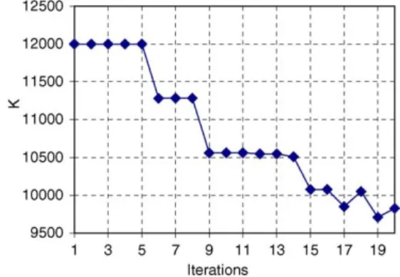
Fig. 3represents the evolution of the objective function andFigs. 4–6represent, respectively, the variation of the co-efficients of the constitutive law K, m and β during the process of optimisation. In iteration 20, the value of the function ob-jective obtained is 8× 10⁻⁵, with K = 9826 Pa s, m = 0.4179
Fig. 3. Convergence of the objective function (the local method).
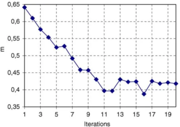
Fig. 5. Evolution of m during the process of optimisation (the local method).
and β = 1553 K. The CPU time is 1 h and 42 min on a com-puter Pentium IV, 2.4 GHz, 512 Mo RAM.
We can choose between precision and CPU time: for ex-ample, in iteration 10, we obtained an error of 6.848× 10⁻³ with a time CPU 51 min; the values of the rheological param-eters are: K = 10,562 Pa s, m = 0.4304, β = 1131 K. With itera-tion 15, we obtained an error of 5.2× 10⁻⁴, with a computing
time of 1 h and 16 min in the same machine, the coefficients obtained are: K = 10,077 Pa s, m = 0.4239 and β = 1350 K.
In Fig. 4, the evolution of the parameter K is shown in function of the iteration. We can see that it is varying quite fast at the beginning of the optimisation, until the ninth step. Its total variation is about 16%.
InFig. 5, the evolution of the parameter m in function of the iteration, we notice that the variation is fast at the beginning of the optimisation, until the 11th step. Its total variation (36%) is more important than for K.
As inFig. 7, the variation of beta in function of iteration step, we can observe that this parameter is quite stable at the beginning and starts to change after iteration 11, when K and
m have almost their final value. 9.2. Result of global response surface
The solution is obtained after six iterations with a precision of 8.4× 10⁻⁴and a CPU time is 1 h and 13 min.Fig. 7
rep-Fig. 6. Evolution of β during the process of optimisation (the local method).
Fig. 7. Convergence of the objective function (the global method).
Fig. 8. Evolution of K during the process of optimisation (the global method).
Fig. 9. Evolution of m during the process of optimisation (the global method).
Fig. 10. Evolution of β during the process of optimisation (the global method).
Table 3
Results of optimisation
h (mm) !P measured (bar) !P (bar) local (1) recalculated Relative error (1) !P (bar) global (2) recalculated Relative error (2)
5 53 52.11 2.8× 10⁻⁴ 49.32 4.8× 10⁻³ 5 99 96.69 5.4× 10⁻⁴ 91.03 6.4× 10⁻³ 5 125 121.6 7.3× 10⁻⁴ 116.8 4.3× 10⁻³ 5 138 132.9 1.3× 10⁻³ 130.4 3.0× 10⁻³ 10 12.7 12.49 2.7× 10⁻⁴ 12.48 3.0× 10⁻⁴ 10 26 25.15 1.0× 10⁻³ 24.89 1.8× 10⁻³ 10 34 34.69 1.2× 10⁻⁴ 34.66 3.7× 10⁻⁴ 10 36.7 39.27 4.9× 10⁻³ 40 8.1× 10⁻³
resents the evolution of the function objective andFigs. 8–10
represent, respectively, the variables of optimisation K, m and β. The optimum parameters are: K = 10,500 Pa s, m = 0.4027 and β = 1194 K.
We can observe that the convergence process is much faster in terms of iteration steps needed. But the computation time is longer. Also, in this method, the three parameters are evolving together in the first iteration steps before reaching values close to the final one.
10. Comparison of the two methods
In Table 3, in function of the operating parameters (slit height, output and temperature), we have reported the pres-sures measured and recalculated using the identified rheolog-ical parameters, so as the relative error (relative difference between the two). We notice that the solution obtained by the method (1) local response surfaces is more accurate, but with an increased computing time. The difference in time be-tween both methods is 30 min. On the other hand, the global response surface method (2) avoids local minimum. This can be improved by varying the design of experiments and the method of approximation to optimise the computing time CPU.
10.1. Pressures
In Fig. 11, the measured pressures and computed pres-sures obtained with the identified rheological parameters are
Fig. 11. Experimental and calculated pressure with parameters determinate by method (2).
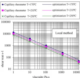
Fig. 12. Computed and measured viscosity method (1).
plotted. There is only a small discrepancy, which means that our method is very robust and gives very good results for both global and local methods. This is also confirmed through the relative error for methods (1) and (2), which are, respectively, 9.14× 10⁻³and 2.9× 10⁻².
10.2. Viscosity
In the graph of viscosity obtained by the coefficients found through the response surface method (Figs. 12 and 13), we can observe that there is no discrepancy between the points of measurements obtained in capillary rheometer and the vis-cosity obtained by the method of optimisation except in the zone, where high shear rates appear.
11. Conclusion and prospects
We conclude that we obtain good results using the re-sponse surface methods (global and local). It means that this method allows us to determine the rheological parameters of polymers directly on a production line. By on will not forced to make measurements on standard capillary rheometers. And also this method will allow us to measure the parameters in industrial conditions, starting from the real geometry even if complex, using pressure measurements, flow rates and tem-peratures.
12. Future works
Also to test the Kriging method[15], we will have to im-prove precision (CPU time) of the global response surface approximation.
We will use the same approximation method to apply on a real 3D geometry to identify the rheological parameters and then to optimise the geometry of die extrusion tolls. The ex-trusion simulations will be processed by using the REM3D®
[16]FEM software.
Acknowledgment
The support of Maillefer-extrusion is gratefully acknowledged.
References
[1] J.F. Agassant, P. Avenas, J.P.H. Sergent, P.J. Carreaur, Poly-mer Processing. Principles and Modelling, Hanser Publishers, 1991.
[2] C. Rauwendahl, Polymer Extrusion, 3rd ed., Hanser Publishers, 1994.
[3] J.-Z. Liang, Characteristics of melt shear viscosity during extrusion of polymers, Polym. Test. 21 (2002) 307–311.
[4] K. Geiger, H. Kuhnle, Analytische Berechnung einfacher scherstro-mungen aufgrund eines fliebgesetzes vom carreauschen typ, Rheog-ica Acta 23 (1984) 355–367.
[5] K.M. Liew, Y.Q. Huang, J.N. Reddy, Vibration analysis of symmetri-cally laminated plates based on FSDT using the moving least squares differential quadrature method, Comput. Methods Appl. Mech. Eng. 192 (2003) 2203–2222.
[6] Y. Krongauz, T. Belytschko, Enforcement of essential bound-ary conditioned in mesh less approximations using finite ele-ments, Comput. Methods Appl. Mech. Eng. 131 (1996) 133– 145.
[7] J. Goupy, Plans d’Exp´eriences Pour Surfaces de R´eponse, Industries Techniques, Paris, 1999.
[8] D. Schl¨afli, Fili`ere Rh´eom´etriques Th´eorie/Fili`ere Plate, Internal Re-port of Nokia Maillefer, 1997.
[9] M.A. Huneault, P.G. Lafleur, P.J. Carreau, Evaluation of the FAN Technique for Profile Die Design, International Polymer Processing, vol. XI, 1996, pp. 50–57.
[10] S.J. Kim, T.H. Kwon, A simple approach to determining three-dimensional screw characteristics in the metering zone of extrusion processes using a total shape factor, Polym. Eng. Sci. 35 (3) (1995) 274–283.
[11] J.M. Renders, Algorithmes G´en´etiques et R´eseaux de Neurones, Herm`es, Paris, 1995.
[12] W. Sun, J. Han, J. Sun, Global convergence of no monotone descent methods for unconstrained optimisation problems, J. Comput. Appl. Math. 146 (2002) 89–98.
[13] J.L. Morales, A numerical study of limited memory BFGS methods, Appl. Math. Lett. (2002) 481–487.
[14] B. Horowitz, S.M.B. Afonso, Quadratic programming solver for structural optimisation using SQP algorithm, Adv. Eng. Software (2002) 669–674.
[15] F. Trochu, P. Terriault, Non-linear modelling of hysteretic material laws by dual Kriging and application, Comput. Methods Appl. Mech. Eng. 151 (1998) 545–558.