Optimal Force Generation of Parallel Manipulators for Passing through the Singular Positions

(1)

HAL Id: hal-00362517

https://hal.archives-ouvertes.fr/hal-00362517

Submitted on 24 Jun 2019

HAL is a multi-disciplinary open access archive for the deposit and dissemination of sci-entific research documents, whether they are pub-lished or not. The documents may come from teaching and research institutions in France or abroad, or from public or private research centers.

L’archive ouverte pluridisciplinaire HAL, est destinée au dépôt et à la diffusion de documents scientifiques de niveau recherche, publiés ou non, émanant des établissements d’enseignement et de recherche français ou étrangers, des laboratoires publics ou privés.

Optimal Force Generation of Parallel Manipulators for

Passing through the Singular Positions

Sébastien Briot, Vigen Arakelian

To cite this version:

Sébastien Briot, Vigen Arakelian. Optimal Force Generation of Parallel Manipulators for Passing through the Singular Positions. The International Journal of Robotics Research, SAGE Publications, 2008, 27 (8), pp.967-983. �hal-00362517�

(2)

Optimal Force Generation in Parallel Manipulators for Passing

through the Singular Positions

Sébastien Briot and Vigen Arakelian

Département de Génie Mécanique et Automatique - L.G.C.G.M. EA3913 Institut National des Sciences Appliquées (I.N.S.A.)

20 avenue des Buttes de Coësmes – CS 14315 F-35043 Rennes, France

E-mails : sebastien.briot@ens.insa-rennes.fr vigen.arakelyan@insa-rennes.fr

Abstract— It is known that a parallel manipulator at a singular configuration can gain one or more degrees of freedom and become uncontrollable. That is it might not reproduce a stable motion along a prescribed trajectory. However, it is proved experimentally that there is possible passing through the singular zones. This was simulated and shown on numerical examples and illustrated on several parallel structures. In this paper, we determine the optimal dynamic conditions generating a stable motion inside the singular zones. The obtained results show that the general condition for passing through a singularity can be defined as follows: the end-effector of the parallel manipulator can pass through the singular positions without perturbation of motion if the wrench applied on the end-effector by the legs and external efforts of the manipulator are orthogonal to the twist along the direction of the uncontrollable motion. This condition is obtained from the inverse dynamics and analytically demonstrated by the study of the Lagrangian of a general parallel manipulator. Numerical simulations are carried out using the software ADAMS and validated by experimental tests.

Index Terms — parallel manipulators, singularity, dynamics, force management, trajectory planning.

(3)

1. Introduction

Parallel manipulators have experienced an increase in popularity in recent years due to their higher rate of acceleration, payload to weight ratio, stiffness and low effective inertia compared to those of serial manipulators. However they have some drawbacks, like a small workspace and special singular zones in it. Thus, in the presence of singular positions, the workspace of the parallel manipulators, which is less than that of serial manipulators, becomes even smaller and limits their functional performance. The studies of singularity have had different stages of development. The previous works on this problem is reported in a great number of publications and can be classified by different criteria. They can be arranged, by example, in three major groups, which are distinguished by historical evolution and are characterized by study of the singularity from kinematic, kinetostatic and dynamic points of view.

The physical interpretation of a singularity in kinematics refers to those configurations of parallel manipulators in which the number of degrees of freedom of the mechanical structure changes instantaneously, either the manipulator gains some additional, uncontrollable degrees of freedom or loses some degrees of freedom. In this case the singularity analysis can be carried out on the base of the properties of the Jacobian matrices of the mechanical structure (i.e. when the Jacobian matrices relating the input speeds and the output speeds become rank deficient (Gosselin and Angeles 1990; Ma and Angeles 1992; Ottaviano, Gosselin and Ceccarelli 2001; Wen and Oapos Brien 2003)), by using Grassmann geometry (Merlet 1989) or screw theory (Bonev, Zlatanov and Gosselin 2003; Hunt 1987). However, it was observed that close to a singular configuration, a parallel manipulator loses its stiffness and its quality of motion transmission, and as a result, its payload capability. For this purpose, a kinetostatic approach has been applied for the evaluation of the quality of motion transmission in the singular zones of

(4)

parallel manipulators. The quality of motion transmission of parallel manipulators was successfully studied in (Kim and Choi 2001; Kim and Ryu 2004; Lee et al. 2002; Weiwei and Shuang 2006). The quality of motion of manipulators with three degrees of freedom has been evaluated by means of a kinetostatic indicator, which is similar to the pressure angle (Alba-Gomez, Wenger and Pamanes 2005). In (Arakelian, Briot and Glazunov 2007), the pressure angle was used as an indicator of the quality of motion transmission and the nature of the inaccessibility of singular zones by parallel manipulators are shown.

The further study of singularity in parallel manipulators has revealed an interesting problem that concerns the path planning of parallel manipulators under the presence of singular positions, i.e. the motion feasibility in the neighborhood of singularities. In this case the dynamic conditions can be considered in the design process. One of the most evident solutions for the stable motion generation in the neighborhood of singularities is to use redundant sensors and actuators (Alvan and Slousch 2003; Collins and Long 1975; Dasgupta and Mruthyunjaya 1998a; Glazunov et al. 2004). However, it is an expensive solution to the problem because of the additional actuators and the complicated control of the manipulator caused by actuation redundancy. Another approach concerns with motion planning to pass through singularity (Bhattacharya, Hatwal and Ghosh 1998; Dasgupta and Mruthyunjaya 1998b; Hesselbach 2004; Kemal Ider 2005; Kevin Jui and Sun 2005; Nenchev, Bhattacharya and Uchiyama 1997; Perng and Hsiao 1999), i.e. a parallel manipulator may track a path through singular poses if its velocity and acceleration are properly constrained. This is a promising way for the solution of this problem. However only a few research papers on this approach have addressed the path planning for obtaining a good tracking performance but they have not adequately addressed the physical interpretation of dynamic aspects.

(5)

In this paper the dynamic condition for passing through the singular positions is defined in general. It allows the stable motion generation inside in the presence of singularity by means of the optimum force control. The disclosed condition can be formulated as follows: «In the presence of a type 2 singularity, the platform of the parallel manipulator can pass through the singular positions without perturbation of motion if the wrench applied on the platform by the legs and external forces is orthogonal to the direction of uncontrollable motion». In other terms, the condition is that the work of applied forces and moments on the platform along the uncontrollable motion is equal to zero. This condition is obtained from the inverse dynamics and analytically demonstrated by the study of the Lagrangian of a general parallel manipulator. The obtained results are illustrated by numerical simulations and validated by experimental tests.

The paper is organized as follows. The next section presents theoretical aspects of the examined problem. Based on the Lagrangian formulation, the condition of force distribution is defined, that allows the passing of any parallel manipulator through the type 2 singular positions. In Section 3, two applications illustrate the obtained theoretical results. In section 4, the numerical simulations carried out using the software ADAMS are validated by experimental tests.

2. Optimal dynamic conditions for passing through type 2 singularity

Let us consider a parallel manipulator of m links, n degrees of freedom and driven by n actuators.

The Lagrangian dynamic formulation for a parallel manipulator can be expressed as:

λ B q q T L L _              dt d  , (1) where,

(6)

- is the vector of the input efforts; - L is the Lagrangian of the manipulator;

- q[q₁,q₂,...,q_n]T and q [q₁,q₂,...,q_n]T represent the vector of active joints variables and the active joints velocities, respectively;

- T z y x, , , , , ] [    x and T z y x, , , , , ] [     

v are trajectory parameters and their derivatives, respectively; x, y, z represent the position of the controlled point and  and  the rotation of the platform about three axes a aand a;

- is the Lagrange multipliers vector, which is related to the wrench applied on the platform by:

p W AT   (2) where,

-A and B are two matrices relating the vectors v and q according toAv Bq. They can be found by the closure equations with respect to time.

-Wp is the wrench applied on the platform by the legs and external forces (Khalil and Guégan

2002), which is defined as:

                         p p p n f x v W L L dt d . (3)

where fp is the force along the directions of the global frame and np is the torque about the axes a aand a

The term Wp can be rewritten in the base frame using a transformation matrix D (Merlet 2006):

) ( 0 p R p D W W  (4)

with R0W_p_{is the expression of the wrench W}

(7)

           3 3 3 3 3 3 3 3 R 0 0 I D (5)

where I33, 033 and R33 are respectively the identity matrix, the zero matrix and the transformation matrix between axes a a and aand the base frame, whose dimensions are 33.

By substituting (5) into (1), one can obtain:

p R b J W W  T 0   , q q Wb             L L  dt d (6)

where J

 

R0A 1B_{is the Jacobian matrix between twist t of the platform (expressed in the base}

frame) and q, R0AAD_{is the expression of matrix A in the base frame.}

For any prescribed trajectory x(t), the values of vectors q , q and q can be found using the inverse kinematics. Thus, taking into account that the manipulator is not in a type 1 singularity (Gosselin and Angeles 1990), the terms Wb and p

R

W

0 _{can be computed. However, for a}

trajectory passing through a type 2 singularity, the determinant of matrix J tends to infinity. Numerically, the values of the efforts applied by the actuators become infinite. In practice, the manipulator either is locked in such a position of the end-effector or it generates an uncontrolled motion. That is the end-effector of the manipulator could produce a motion, different to the prescribed trajectory.

It is known that a type 2 singularity appears when the determinant of matrix R0A_{vanishes, in}

other words, when at least two of its columns are linearly dependant (Merlet 2006). Let us rewrite the matrix R0A_as:

             66 62 61 26 22 21 16 12 11 0 a a a a a a a a a        A R (7)

(8)

In the presence of type 2 singularity the columns of matrix R0A_{are linearly dependant, i.e.}



  6 1 0 j ij ja  , i = 1, …, 6 (8)

where j are the coefficients, which in general can be functions of qp (p = 1, …, n). It should be

noted that the vector ts = 2, …, 6]T represents the direction of the uncontrollable motion of the platform in a type 2 singularity.

Rewriting (8) in a vector form, we obtain:



  6 1 j j jN 0  , Nj = [a1j, a2j, …, a6j]T, j = 1, …, 6 (9) where Nj represents the j-th column of matrix R0A.

By substituting (9) into (2), we obtain

j T

jλW

N , j = 1, …, 6 (10)

where Wj is the j-th row of vector p R

W

0 _.

Then, from (9) and (10) the following conditions are derived:











    6 1 6 1 0 j j j j T j j W  N λ (11)

The right term of eq.(11) corresponds to the scalar product of vectors ts and R0W_p_.

Thus, in the presence of a type 2 singularity, it is possible to satisfy conditions (11) if the

wrench applied on the platform by the legs and external efforts R0W_p_{are orthogonal to the}

direction of the uncontrollable motion ts. Otherwise, the dynamic model is not consistent.

Obviously, in the presence of a type 2 singularity, the displacement of the end-effector of the manipulator has to be planned to satisfy (11).

(9)

3. Illustrative examples

In this section, two examples are chosen to illustrate the obtained theoretical results discussed above. The first example presents a planar 5R parallel manipulator, which allows obtaining relatively simple mathematical models for demonstrating the expected results by numerical simulations. The second example presents a parallel manipulator which was developed in the I.N.S.A. of Rennes. This example was chosen for validation of numerical simulations carried out by the software ADAMS on the built prototype.

3.1. Example 1: Planar 5R parallel manipulator

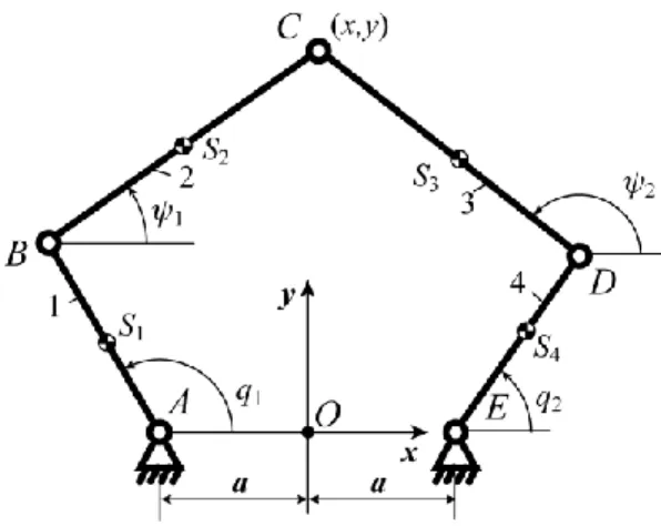
In the planar 5R parallel manipulator, as shown in Fig. 1, the output point is connected to the base by two legs, each of which consists of three revolute joints and two links. In each of the two legs, the revolute joint connected to the base is actuated. Thus, such a manipulator is able to position its output point in a plane.

(10)

(a)1 = 2  (b)1 = 2

Fig. 2. Second kind of singularities of the planar 5R parallel manipulator.

As shown in Fig. 1, the actuated joints are denoted as A and E with input parameters q1 and q2. The common joint of the two legs is denoted as C, which is also the output point with controlled parameters x and y. A fixed global reference system xOy is located at the center of AE with the y-axis normal to AE and the x-y-axis directed along AE. The lengths of the links AB, BC, CD, DE are respectively denoted as L1, L2, L3 and L4. The positions of the centers of masses Si of links from

joint centers A, B, D and E are respectively denoted by dimensionless lengths r1, r2, r3 and r4, i.e.

1 1

1 rL

AS  , BS2 r2L2, DS3 r3L3 and ES4 r4L4.

The singularity analysis of this manipulator (Liu, Wang and Pritschow 2006) shows that the Type 2 singularities appear when legs 2 and 3 are parallel (Fig. 2).

In both cases, the gained degree of freedom is an infinitesimal translation perpendicular to the legs 2 and 3. However, if L2 = L3, the gained degree of freedom in case (b) becomes a finite rotary motion about point B.

In order to simplify the analytic expressions, we consider that the gravity effects are along the

z-axis and consequently the input torques are only due to inertia effects. To simplify the

(11)

(Seyferth 1974; Wu and Gosselin 2007). For a link i with mass mi and its axial moment of inertia Ii, we have:                                  i i i i i i i i i i i I m m m m L r L r r r 0 ) 1 ( 0 1 0 1 1 1 3 2 1 2 2 2 2 , (i = 1, 2, 3, 4) (12)

where mij (j = 1, 2, 3) are the values of the three point masses placed at the centers of the revolute

joints and at the center of masses of the link i. In this case, the kinetic energy T can be written as:

) ( 2 1 2 2 2 2 4 4 2 3 3 2 2 2 2 1 1 S S S S S S S B B C C D D S m m m m m m m T  V  V  V  V  V  V  V (13) where, m_S₁ m₁₂, m_S₂ m₂₂, m_S₃ m₃₂, m_S₄ m₄₂, m_B m₁₃m₂₁, m_C m₂₃m₂₁, 41 33 m m

m_D   . The terms mij (i = 1, 2, 3, 4) are deduced from the relation (12), VSi is the vector

of the linear velocities of the center of masses Si; VB, VC and VD are the vectors of the linear

velocities of the corresponding axes.

The input torques can be obtained from (6):

p

b J W

W  T₅_R



 (14)

taking into account that for examined manipulator:

D D B B b J F J F W  T  T , (15) where,        0 cos 0 sin 1 1 1 1 q L q L B J , _        2 4 2 4 cos 0 sin 0 q L q L D J , (16) C B B F m_B₁ m_C₁ , F_D m_D₂_Dm_C₃_C, (17)                     1 1 2 1 1 1 1 1 sin cos cos sin q q q q q q L   B  , _                    2 2 2 2 2 2 2 4 sin cos cos sin q q q q q q L   D  , _       y x     C  (18)

(12)

2 2 2 2 1 1 1 m r m m (1 r ) m_B  _S  _B _S  , m_C₁m_S₂r₂(1r₂), (19) ) 1 ( ₃ 3 3 3 m r r m_C  _S  , m_D₂ m_S₄r₄2 m_D m_S₃(1r₃)2. (20) The term Wp is given by:

D C B p W m_C₁ m_C₂ m_C₃ , (21) 2 3 3 2 2 2 2 m r m m r m_C  _S  _C  _S . (22)

and the Jacobian matrix J5R by:

R R R 5 1 5 5 A B J   , (23) where,                     2 4 2 4 1 1 1 1 22 21 12 11 5 sin cos sin cos 2 q L y a q L x q L y a q L x a a a a R A , (24)           ) cos sin ( 0 0 ) cos sin ( 2 22 2 21 4 1 12 1 11 1 5 q a q a L q a q a L R B . (25)

and we determine ts in according with (8):

T ] cos , sin [ ₁ ₁  s t (26)

Thus, the examined manipulator can pass through the given singular positions if the wrench

Wp determined by (21) is orthogonal to the direction of the uncontrollable motion ts described by

(26).

Let us now consider the motion planning, which makes it possible to satisfy this condition. For this purpose the following parameters of manipulator’s links are specified: L1 = L2 = L3 = L4 = 0.25 m; r1 = r2 = r3 = r4 = 0.5; a = 0.2 m; m1 = m4 = 2.81 kg; I1 = I4 = 0.02 kg/m2; m2 = m3 = 1.41 kg; I2 = I3 = 0.01 kg/m2.

(13)

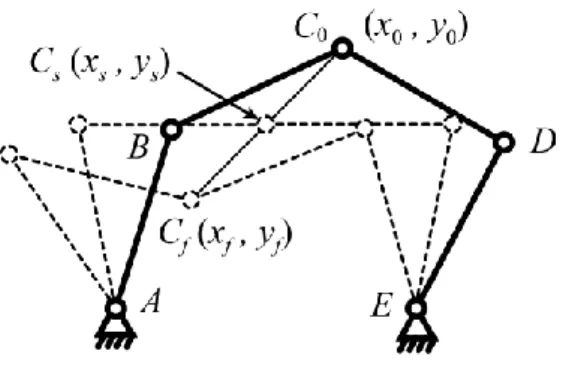
Fig. 3. Initial, singular and final positions of the planar 5R parallel manipulator.

With regard to the prescribed trajectory generation, the point C should reproduce a motion along a straight line between the initial position C0 (x0, y0) = C0 (0.1, 0.345) and the final point Cf

(xf, yf) = Cf (-0.1, 0.145) in tf = 2 s.

Thus, the given trajectory can be expressed as follows:

                  ) ( ) ( ) ( ) ( ) ( ) ( 0 0 0 0 y y t s y x x t s x t y t x f f x (27)

However, the manipulator will pass by a type 2 singular position at point Cs (xs, ys) = Cs (0,

0.245) (Fig. 3).

Developing the condition for passing through the singular position (11) for the planar 5R parallel manipulator at point Cs, we obtain:

0 6 3 ) 48 248 ( 2 2 ₂ 1 1L x  y  m y m_C   _C  (28)

Then, taking into account that the velocity and the acceleration of the end-effector in initial and final positions are equal to zero, the following nine boundary conditions are found:

s (t0) = 0, (29)

s (tf) = 1, (30)

(14)

0 ) (t₀  s , (32) 0 ) (t_f  s , (33) 1 ) /( ) /( ) (t  y y y₀ x x x₀  s _s _s _f _s _f , (34) 0 ) (t₀ s₀  s   . (35) 0 ) (t_f s_f  s   . (36) ) 6 ) ( 3 /( ) 48 248 ( ) (t_s s_s m_C₁L₁ x_s2 y_s2 x_f x₀ m_C₂ s        . (37)

(a) actuator 1 (b) actuator 2

Fig. 4. Input torques of the planar 5R parallel manipulator in the case of the eight order polynomial trajectory planning, obtained by the ADAMS software.

(15)

(a) actuator 1 (b) actuator 2

Fig. 5. Input torques of the planar 5R parallel manipulator in the case of the fifth order polynomial trajectory planning, obtained by the ADAMS software.

From (28) – (37), the following eighth order polynomial trajectory planning is found:

 

3 4 5 6 7 8 12606 . 0 07101 . 1 58909 . 3 72792 . 5 84228 . 3 25851 . 0 t t t t t t t s       (38)

Thus the generation of the motion by the obtained eighth order polynomial makes it possible to pass through the singularity without perturbation and the input torques remain in the limits of finite values, which are validated by numerical simulations carried out by the ADAMS software (Fig. 4).

Thus, we can assert that the obtained optimal dynamic conditions assume the passing of the manipulator’s end-effector through the singular position.

Now, we would like to show that, in the case of the generation of the motion by any trajectory planning without meeting the adopted boundary conditions, the end-effector is not able to pass through the singular position. For this purpose the generation of motion between initial and final positions, let us generate by a fifth order polynomial trajectory planning:

 

3 4 5 1875 . 0 9375 . 0 25 . 1 t t t t s    (39)

(16)

The obtained numerical simulations carried out by the software ADAMS are given in Fig. 5. We can see that, when the manipulator is close to the singular configuration (for ts = 1 s), the

values of the input torques tend to infinity.

3.2. Example 2: PAMINSA (Parallel Manipulator of the I.N.S.A.)

The second example presents a parallel manipulator, which was invented and developed at the I.N.S.A of Rennes (Arakelian et al. 2006). The particularity of this architecture is in decoupling of the displacements of the platform in the horizontal plane from the translations along the vertical axis. The advantages of such an approach was disclosed in (Arakelian et al. 2005; Briot et al. 2007b) and the singularity analysis is discussed in (Briot et al. 2007a; Briot and Arakelian 2007; Arakelian, Briot and Glazunov 2006).

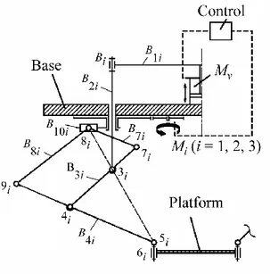
The previous studies have revealed that there are type 2 singularities in the workspace of the symmetrical architecture of PAMINSA. Let us illustrate the proposed approach for the PAMINSA with 4 degrees of freedom (Fig. 6).

Each leg of this manipulator is realized by a pantograph mechanism (Fig. 7) with two input points 3i and 8i, and an output point 5i (i = 1, 2, 3). Each input point 8i is connected to the rotating

drive Mi by means of a prismatic guide mounted on a rotating link. This kind of architecture

allows for generation of motion in the horizontal plane by the use of rotating actuators M1, M2,

M3, and the vertical translations by means of the linear actuator Mv. Thus, the displacements (x, y,

) of the platform in the horizontal plane xOy, that are translations along the x and y-axes and rotations about the z-axis, are independent of vertical translations z.

(17)

Fig. 6. PAMINSA with 4 DOF.

Fig. 7. Kinematic chain of each leg.

This implies that the kinematic models controlling the displacement of the manipulator can be divided into two parts:

- a model for the displacements in the horizontal plane, which is equivalent to a 3-RPR manipulator;

(18)

- a model for the translations along the vertical axis equivalent to the model for the vertical translations of a pantograph linkage.

The type 2 singularities of such a manipulator appear when (Arakelian, Briot and Glazunov 2006; Briot et al. 2007a):

a) the three legs of the manipulators are parallel, which is impossible for the developed PAMINSA manipulator.

b) the orientation of the platform is equal to cos1(R_pl/R_b), where Rpl and Rb correspond

respectively to the lengths PCi and OM’i (Fig. 8). In this case, the manipulator gains one

infinitesimal rotation around one vertical axis. c) the platform is located in a circle defined by

x2  y2 R_pl2 R_b2 2R_plR_bcos (40) In this case, the manipulator gains one finite rotation about one vertical axis (Cardanic self motion) (Briot et al. 2007a).

Fig. 8. Example of Type 2 singular configuration (horizontal projection of the examined structure).

(19)

For both cases (b) and (c), the direction of the unconstrained motion can be represented by the twist ts = [0, 0, 1, xW, yW, 0]T, where xW and yW corresponds to the planar coordinates of the

intersection point of the wrenches Ri applied on the platform by the three legs of the manipulator

(Fig. 8).

Let us now study the inverse dynamics of the PAMINSA. The potential energy V can be written as:



   3 1 i leg pl V i V V (41)

where Vpl is the potential energy of the platform and Vleg_iis the potential energy of the leg i (i = 1,

2, 3).

By further considering that the coordinates of the all points of the pantograph linkages can be found as a linear combination of the coordinates of points 3i, 5i and 9i, one can express the terms

Vpl and Vleg_i as follows:

z g m V_pl  _pl (42) 4 3 9 2 5 1 i v i v v v v leg C z C z C q C V i     (43)

Here, Cvj (j = 1, 2, 3) are constant terms whose dimension is equivalent to a mass multiplied by

the gravitational acceleration g, mpl is the mass of the platform with a payload, and z5i and z9i are the altitude of joints 5i and 9i. The expressions of the coordinates of joints 5i and 9i are given in

appendix A. The expressions for Cvj (j = 1, …, 4) are given in appendix B.

We consider that the links are perfect tubes. Therefore the tensor of inertia Ij of the link Bji at

(20)

           ) ( ) ( ) ( 0 0 0 0 0 0 j ZZ j YY j XX j I I I I , with I_YY(j) I_ZZ(j) (44)

Thus, the kinetic energy T of the manipulator can be represented as:



   3 1 i leg pl T i T T , (45)

where Tpl is the kinetic energy of the platform, Tlegi is the kinetic energy of the leg i, as:



2 2 2 2



) ( 2 1 __    _pl pl pl m x y z I T     (46)

where Ipl is the axial moment of inertia of the platform about the vertical axis.

i i i trans rot leg T T T   (47) 2 8 5 7 6 9 5 5 9 5 9 5 4 2 9 2 9 2 9 3 2 5 2 2 5 2 5 1( ) ( ) ( ) i c v i c v c i i c i i i i c i i i c i c i i c trans q C q z C q C z z C y y x x C z y x C z C y x C T i                             (48) i rot

T is the kinetic energy of the rotating links.

Note that there are two types of rotations (see, Fig. 7):

- rotation due to the actuators Mi (i = 1, 2, 3) (angle qi), which is about the vertical axis,

- rotations due to the displacement of the pantograph in the linkage plane (angles i and i

denoted as the angles between the direction of the passive slider and the links B4i and B3i respectively).

Thus, the kinetic energy of the rotating links can be written as:

) cos sin cos sin ( 2 11 2 12 2 9 2 10 13 2 2 10 2 9 i c i i c c i c i c i c i c rot C C q C C C C C T i                ₍₄₉₎

The expressions for Ccj (j = 1, …, 13) are given in appendix C.

The input torques can be obtained from (6):

p

b J W

W  T_PAM



(21)

where the terms JPAM, Wb and Wp are presented in appendix D.

The following parameters of manipulator’s links are specified for the trajectory generation: - the radii of the circles circumscribed to the base and platform triangles are respectively equal

to Rb = 0.35 m and Rpl = 0.1 m;

- magnification factor of the pantograph: k = 3; - gravitational acceleration g is equal to 9.81 m/s2

.

- lengths of the links of the pantograph linkages: LB1 = 0.308 m, LB2 = 0.442 m, LB3 = LB8 = 0.42

m, LB4 =k LB7 = 0.63 m, LB5 = 0.0275 m, LB10 = 0.3635 m;

- masses of the joints of the pantograph linkages: m2 = 0.214 kg, m3 = 0.338 kg, m4 = 0.262 kg,

m5 = 0.233 kg, m7 = 3.08 kg, m8 = 0.305 kg, m9 = 0.259 kg; - mass of the platform: mpl = 2.301 kg;

- masses of the links of the pantograph linkages: mB1 =1.221 kg, mB2 = 0.921 kg, mB3 = 0.406 kg,

mB4 = 0.672 kg, mB7 = 0.107 kg, mB8 = 0.403 kg, mB10 = 0.436kg;

- term of the inertia matrix of the platform: 2

kg/m 015 . 0  pl I .

- terms of the inertia matrices of the links of the pantograph linkages:

2 ) 3 ( kg/m 0038 . 0  B XX I , ( 3) 2 kg/m 02 . 0  B YY I , ( 4) 2 kg/m 0012 . 0  B XX I , ( 4) 2 kg/m 048 . 0  B YY I , 2 4 ) 7 ( kg/m 10 8   B XX I , ( 7) 2 kg/m 003 . 0  B YY I , ( 8) 2 kg/m 0024 . 0  B XX I , ( 8) 2 kg/m 02 . 0  B YY I , 2 2 0.003kg/m B I , 2 10 0.02kg/m B I .

The point P is desired to make a motion x(t) along a straight line between points P0 (x0, y0) = P0 (0, 0) and point Pf (xf, yf) = Pf (0.3, 0) in tf = 2.4 s. However, the manipulator will pass through a

(22)

Fig. 9. Displacement of the PAMINSA along the prescribed straight line (planar projection).

In order to carry out a comparative analysis for the optimized and not optimized dynamic conditions for passing through type 2 singularity, it has been considered two cases. The first is such a movement on the given trajectory, which is calculated from condition (11), and the second is an arbitrary motion.

At first let us consider an optimized trajectory which allows satisfying the condition (11), i.e. the force Wp should be perpendicular to the to the twist ts [0, 0, 1, 0, 0.1, 0]T defining the

direction of the unconstrained motion. Developing the expression (11) for the PAMINSA at point Ps, we obtain: z y z x y x z y x z y x z y x                         94694 . 2 46477 . 0 17625 . 5 19423 . 0 05643 . 0 85175 . 0 02947 . 0 18482 . 0 11720 . 0 85084 . 6 06827 . 0 04425 . 0 14649 . 0 2115 . 1 06441 . 0 0 2 2 2 2                     (51)

Now considering that the end-effector of the manipulator moves along a straight line directed along the x-axis, we can note that y(t_s) = z(t_s) = y(t_s) = z(t_s) = (t_s) = (t_s) = 0. Thus, the relationships, which satisfy the passing through of the singular positions, taking into account that

(23)

the velocity and the acceleration of the platform in the initial and final positions are equal to zero, can be expressed by the following boundary conditions:

x(t0) = x0, (52) x(tf) = xf, (53) x(ts = 2s) = xs, (54) 0 ) (t₀  x , (55) 0 ) (t_f  x , (56) 0 ) (t₀  x  , (57) 0 ) (t_f  x  , (58) 05 . 0 ) (t_s x_s  x  m/s, (59) 1.32583 ) (t_s x_s  x   m/s². (60)

In this case, a motion for passing of the platform through the singular position can be found from the following eighth order polynomial form:

 

8 7 6 5 4 3 27 . 175 63 . 400 23 . 365 05 . 166 65 . 37 41 . 3 t t t t t t t x       (61)

However, a trajectory obtained by (61) cannot be reproduced by the prototype because of the limited capability of drivers’ deceleration. Therefore, the trajectory was divided into two parts, i.e., the first sixth order polynomial trajectory assumes the motion from an initial to the singular position (P0Ps) and the second sixth order polynomial trajectory from singular to the final

position (PsPf). The core of the problem is same but it allows for generating motions for the

prototype.

Thus, the trajectory planning equations can be written as:

 





It can be seen that the input torques remain in the limits of finite values, but, by the end of the motion there is an increase of the input efforts, caused by a quick deceleration to stop the manipulator before it reaches the workspace boundary. It will be shown further that in the case of the motion generated by any trajectory planning without meeting the adopted boundary conditions (52) – (60), the manipulator platform is not able to pass through the singular position. For this purpose, the generation of motion between initial and final positions is carried out by a fifth order polynomial trajectory planning.

In this case, fory

 

t 0m, z

 

t 0.45mand

 

t 0, the fifth order polynomial trajectory planning is the following:

 

3 4 5 023 . 0 137 . 0 217 . 0 t t t t x    (66)

The obtained input efforts computed by the software ADAMS are represented in Fig. 11. It can be noted that, while the manipulator passes through the singular configuration (for ts ≈

1.8 s), the value of the input torques tend to infinity.

(25)

(a) actuator M1 (b) actuator M2

(c) actuator M3

Fig. 10. Input efforts of the PAMINSA in the case of the sixth order polynomial trajectory planning, computed with ADAMS software.

(26)

(a) actuator M1 (b) actuator M2

(c) actuator M3

Fig. 11. Input efforts of the PAMINSA in the case of the fifth order polynomial trajectory planning, computed with ADAMS software.

(27)

4. Experimental validation of obtained results

For validating the results of the previous section, we have carried out experimental tests on the prototype of the PAMINSA developed in the I.N.S.A. of Rennes (Fig. 12).

Fig. 12. The prototype of PAMINSA developed in the I.N.S.A. of Rennes.

Fig. 13. Trajectory reproduction on the PAMINSA during the displacement of the platform with the fifth order polynomial law (view from below).

(28)

Fig. 14. Trajectory reproduction on the PAMINSA during the displacement of the platform with the sixth order polynomial law (view from below).

At first, we have applied an arbitrary fifth order control law and observed the reproduction of motion during the displacement of the platform. The obtained trajectory is shown in Fig. 13 (dotted line).

The different positions are classified by time. For positions from (a) to (d), the platform moves towards the singular zone but yet it is outside of it. In this case, the reproduction of the real trajectory is similar to the desirable. At position (e), the manipulator enters the singular zone, which is close to the circle of the theoretical singular loci, and starts an uncontrollable motion. Thus, since the motion generation is carried out by non optimized dynamic parameters, the platform moves along an unplanned trajectory (see positions (e) - (h) in Fig. 13).

Next, we have implemented the sixth order control laws as it was shown in the previous section and observed the behavior of the platform during the displacement (Fig. 14). The different positions are classified by time. During all these displacements, the manipulator retains its orientation and passes through the singular configuration without any perturbation.

(29)

Thus, we can note that the obtained optimum dynamic conditions allow the passing of the manipulator through the singular position.

5. Conclusion

At a singular configuration, a manipulator can gain one or more degrees of freedom, and at such a configuration it may becomes uncontrollable, i.e. it may not reproduce stable motion with prescribed trajectory. Nevertheless it is approved that there are several motion planning techniques, which allow passing through these singular zones. These approaches are simulated by numerical examples and illustrated on several parallel structures. It is a promising tendency for the solution of this problem. However, the attention was focused only on control aspects of this problem and very little attention has been paid to the dynamic interpretation, which is a crucial factor for governing the behavior of parallel manipulators at the singular zones.

In this paper we have found the optimal dynamic conditions, for making the pass through the type 2 singular configurations possible. The general definition of the condition for passing through the singular position is formulated as follows: in the presence of type 2 singular configuration, the platform of a parallel manipulator can pass through the singular positions without perturbation of motion if the wrench applied on the platform by the legs and external efforts are orthogonal to the direction of the uncontrollable motion, or in other words, if the work of applied forces and moments on the platform along the uncontrollable motion is equal to zero. This condition has been verified by numerical simulations carried out with the software ADAMS and validated by experimental tests on the prototype of four degrees of freedom parallel manipulator PAMINSA.

(30)

It should be noted that the formulated general conditions ensure any given trajectory generation in the manipulator workspace. We would like to point out that the trajectory is not imposed and only the conditions of force generation must be satisfied.

Thus, the passing of any parallel manipulator through the singular positions by the proposed technique is carried out by optimal generation of inertia forces. Hence, it is impossible to stop the manipulator in the singular locus and to start again from fixed position.

We would like to mention that we studied the optimal redistribution of forces only in singular positions of the manipulator but it should be noted that there are zones close to these positions, in which the manipulator loses the quality of motion. For more reliable generation of motion, it is desirable to ensure the given condition of force generation not only in the singular positions of the manipulator but also in the zones near to these positions. It should be also mentioned that a future development of our work is the study of the difficulties of controlling parallel robots in the neighbourhood of singular configurations.

Finally, it should be noted that for the case of non controllable external forces applied on the platform the proposed technique cannot be used. Therefore, the most prominent field of the industrial application is a “fast pick and place” manipulation, when the generation of motion is determined by input, gravitational and inertia forces.

APPENDIX A

Coordinates of points 3i, 5i and 9i (i = 1, 2, 3):

                     k z R R z y x i i b i b i i i / sin cos 5 3 3 3   ,                                   c i pl i pl i i i L R R z y x z y x ) sin( ) cos( 5 5 5     , where i = (-5/6, -/6, /2),

(31)

                       F q X y q X x z y x i i i i i i i i i sin cos 9 3 9 3 9 9 9 with: F B A X₉_i   , F (DK)/(2E), K D2 4EC, E(B21), D2B(X₈_i A), 2 8 2 8 2 3 X 2AX A L C _B  _i  _i  , Bz5i/(kX8i), ( )/(2 8 ) 2 5 2 8 2 5 2 3 2 4 B i i i i B L X X z kX L A     , ) 1 /( 5 8 X k X _i _i , X₅_i  (x₅_i x₃_i)2(y₅_i y₃_i)2 . APPENDIX B Expressions of terms Cvj (j = 1, …, 4):                               



2,3,4,7 1,7  3 2 4 5 1 2 2 j j j Bj Bj B j v k m k m m k m m g C ,                2 2 ) 2 ( ) 1 ( ₄ ₇ ₉ ₃ ₇ ₄ ₈ 2 B B B B v m m k m m k k m k m m k g C , 2 1 3 B v m g C  ,          2 2 1 2 2 4 B B B v m m m L g C . APPENDIX C Expressions of terms Ccj (j = 1, …, 13):                      8 ₂ 2 2 7 4 2 2 3 2 8 2 7 5 2 4 1 )) 1 ( 2 ( )) 1 ( 2 ( ) 1 ( 4 )) 1 ( 2 ( ) 2 ( ) 1 ( )) 1 ( ( 2 1 k m k k k m m k k k m k m k k m m k m C B B B B c                               



   4 4 2 1 3 ₄ 2 2 7 , 1 2 5 7 , 4 , 3 , 2 2 2 B j Bj j Bj j j c m k m k m m k m C                4 4 4 4 ) 2 ( ) 1 ( 2 1 ₈ 2 7 4 2 2 3 9 2 7 2 4 2 3 B B B B c m k m m k k m m k m k m k C

(32)

                   ) 1 ( 2 ) 1 ( 2 ) 1 ( 2 ) 1 ( 2 ) 2 ( ) 1 ( ) 1 ( 2 2 1 8 2 7 4 2 2 3 2 7 2 4 4 k m k k k m m k k k m k k m k m k C B B B B c              2 2 ) 2 ( 2 ) ) 1 (( 4 2 1 ₄ 2 3 7 7 4 5 B B B c m k k m m m m k C 8 1 6 B c m C  , k m C B c 4 1 7  , 8 2 10 10 8 B B c L m C  , 2 ) 7 ( ) 4 ( 9 B YY B YY c I I C   , 2 ) 7 ( ) 4 ( 10 B XX B XX c I I C   , 2 ) 8 ( ) 3 ( 11 B YY B YY c I I C   , 2 ) 8 ( ) 3 ( 12 B XX B XX c I I C   , 2 10 2 13 B B c I I C   . APPENDIX D

JPAM = A-1B is the global Jacobian matrix where matrice A and B are:

                                        0 1 0 0 0 1 0 0 0 1 0 0 sin cos 0 cos sin sin cos 0 cos sin sin cos 0 cos sin 3 3 2 2 1 1 3 3 3 3 3 3 2 2 2 2 2 2 1 1 1 1 1 1 PC PC PC PC PC PC T PC PC T PC PC T PC PC x y x y x y q z q z q q q z q z q q q z q z q q 3 3 2 2 1 1 d PC d PC d PC A ,                      k k k 0 0 0 0 0 0 0 0 0 0 0 0 0 0 0 0 0 0 3 2 1    B with 5 3 2 2 3 5 ) ( ) ( _i _i _i _i i  x x  y y  ,



 



T i i i T PCi PCi PCi y z x x y y z z x      , , ₅ , ₅ , ₅ i

PC and d_i 



cosq_i sinq_i 0



T (for i = 1, 2, 3). The expressions of the terms Wb and Wp are:

(33)

) ( 2 2 10 10 7 7 8 8 3 3 4 4 3 1 2 2 7 7 9 9 4 4 3 3 i S T i S i S T i S i S T i S i S T i S i S T i S i S T i S i i T i i T i i T i i T i i T i F J F J F J F J F J F J F J F J F J F J F J W Q Q Q Q Q Q Q Q Q Q Q b           



 ) ( 7 7 8 8 3 3 4 4 7 7 3 1 4 4 9 9 5 5 8 8 i S T i S i S T i S i S T i S i S T i S i T i i i T i i T i i T i i T i F J F J F J F J F J F J F J F J F J F W X X X X X X X X X P p          



 with                                  1 3 3 3 3 3 1 3 3 3 3 3 X 0 0 0 0 J  T i i i T T i i i i z y x z y x z y x [ , , ] ] , , [ ] , , [ ₅ ₅ ₅ ₅ ₅ ₅ 5 , 8i _k 0 1 5i 0 1 1 1 X 4 4 1 4 1 4 4 1 4 1 X J 0 0 0 0 0 J                  ,                 1 3 3 3 3 1 1 2 3 2 Q 0 0 0 0 0 J 3i 1 , JQ2i JQ3i, T T B i qi i T B i qi i T B i qi i i L L L                                                                      3 1 3 1 1 2 P 3 1 1 2 P 3 1 1 2 P 3 1 Q 0 0 0 Rot R 0 0 Rot R 0 0 Rot R 0 J 3 3 3 2 3 1 9 ) , ( ) , ( ) , ( y y y       ,               0 0 0 0 sin cos 0 cos sin i i i i qi q q q q P R , i i i B i i i L q 8 3 ε 9 ) , ( X X 1 3 1 3 1 3 1 2 P X J J 0 0 0 0 R Rot J                        z ,               i i i i i     sin 0 cos 0 0 0 cos 0 sin ε P R ,

(34)





                   i i i B i B i B i B i i k k L L L L 5 1 4 3 4 3 1 1 cos cos sin sin X 3 1 2 1 X X J 0 0 J J __      ,                     i i i i i z y x 0 0 X J , _i T T B i qi i T B i qi i T B i qi i i k L k L k L 9 4 3 4 2 4 1 4 / ) , ( / ) , ( / ) , ( Q 3 1 3 1 1 2 P 3 1 1 2 P 3 1 1 2 P 3 1 Q J 0 0 0 Rot R 0 0 Rot R 0 0 Rot R 0 J                                                                       y y y       , i i i B i i i k L q 9 4 4 / ) , ( X X 1 3 1 3 1 2 P 1 3 X J J 0 0 0 R Rot 0 J                          z ,               i i i i i      sin 0 cos 0 0 0 cos 0 sin P R , T T B i qi i T B i qi i T B i qi i i k L k L k L                                                                      3 1 3 1 1 2 P 3 1 1 2 P 3 1 1 2 P 3 1 Q 0 0 0 Rot R 0 0 Rot R 0 0 Rot R 0 J / ) , ( / ) , ( / ) , ( 4 3 4 2 4 1 7 y y y       , i i i B i i i k L q 8 4 7 / ) , ( X X 1 3 1 3 1 2 P 1 3 X J J 0 0 0 R Rot 0 J                          z ,





_           i i i i S 1 Q 4 3 Q Q Q J 0 J J J ₄ 0.5 ₅ ₉ ,             0 3 2 1i i i i    1 2 1 2 1 2 1 2 1 Q 0 0 0 0 J ,





_          i i i i S 1 Ω 9 5 4 0.5 X 6 3 X X X J 0 J J J , _i _i_i i i q q   X 1 X J J              0 0 cos 0 sin 0 ,





_T



T Sji Sji B Sji Bj Sji Bj Bji m x m y m z C F    ₂ , for j = 3, 4, 7, 8

















Bji T i i Bj i i Bji T i i i qi Bj i i Bji T i i Bj i i i qi Sji q q q q q q     ) , ( ) , ( ) , ( ) , ( ) , ( ) , ( ) , ( ) , ( ) , ( ) , ( ) , ( ) , ( y Rot z Rot I y Rot z Rot R z Rot y Rot R I y Rot z Rot y Rot z Rot I R z Rot y Rot R C P P P P              with i = i if j = 4, 7, i = i if j = 3, 8 and





T i i i i i

Bji   sinq  cosq q

Ω .

(36)

REFERENCES

Alba-Gomez, O., Wenger, P., and Pamanes, A., 2005, September 24-28, “Consistent kinetostatic indices for planar 3-DOF parallel manipulators, application to the optimal kinematic inversion,” Proc. ASME 2005 IDETC/CIE Conference, Long Beach, California.

Alvan, K., and Slousch, A., 2003, “On the control of the spatial parallel manipulators with several degrees of freedom,” Mechanism and Machine Theory, Saint-Petersburg, No. 1, pp. 63-69.

Arakelian, V., Briot, S., Guegan, S., and Le Flecher, J., 2005, November 29 – December 1, “Design and prototyping of new 4-, 5- and 6-DOF parallel manipulators based on the copying properties of the pantograph linkage,” Proc. 36th International Symposium on Robotics, Tokyo, Japan.

Arakelian, V., Briot, S., and Glazunov, V., 2006, “Singular positions of a PAMINSA parallel manipulator,” Journal of Machinery Manufacture and Reliability, Allerton Press Inc., No 1, pp. 62-69.

Arakelian, V., Maurine, P., Briot, S., and Pion, E., 2006, January 27, “Parallel robot comprising means for setting in motion a mobile element split in two separate subassemblies,” FR2873317 (A1), WO 2006/021629.

Arakelian, V., Briot, S., and Glazunov, V., 2007, “Increase of singularity-free zones in the workspace of parallel manipulators using mechanisms of variable structure,” Mechanism and Machine Theory, in press.

Bhattacharya, S., Hatwal, H., and Ghosh, A., 1998, “Comparison of an exact and approximate methode of singularity avoidance in platform type parallel manipulators,” Mechanism and Machine Theory, Vol. 33, No. 7, pp. 965-974.

(37)

Bonev, I.A., Zlatanov, D., and Gosselin, C.M., 2003, “Singularity analysis of 3-DOF planar parallel mechanisms via Screw Theory,” Transactions of the ASME. Journal of Mechanical Design, Vol. 125, pp. 573-581.

Briot, S., and Arakelian, V., 2007, June 17-21, “Singularity Analysis of PAMINSA Manipulators,” Proc. 12th

World Congress in Mechanism and Machine Science, Besançon, France.

Briot, S., Bonev, I.A., Chablat, D., Wenger, P., and Arakelian, V., 2007, “Self Motions of General 3-RPR Planar Parallel Robots,” The International Journal of Robotics Research, in press.

Briot, S., Guegan, S., Courteille, E., and Arakelian, V., 2007, September 4-7, “On the Design of PAMINSA: a New Class of Parallel Manipulators with High-Load Carrying Capacity,” Proc. ASME 2007 IDETC/CIE Conference, Las Vegas, Nevada, USA.

Collins, C.L., and Long, G.L., 1975, “The singularity analysis of an parallel hand controller for force-reflected teleoperation,” IEEE Transactions on Robotic and Automation, Vol. 11, No. 5, pp. 661-669.

Dasgupta, B., and Mruthyunjaya, T., 1998, “Force redundancy in parallel manipulators: theoretical and practical issues,” Mechanism and Machine Theory, Vol. 33, No. 6, pp.724-742.

Dasgupta, B., and Mruthyunjaya, T., 1998, “Singularity-free path planning for the Steward platform manipulator,” Mechanism and Machine Theory, Vol. 33, No. 6, pp. 715-725. Gosselin, C.M., and Angeles, J., 1990, “Singularity analysis of closed-loop kinematic chains,”