HAL Id: hal-00824670
https://hal.archives-ouvertes.fr/hal-00824670
Submitted on 22 May 2013
HAL is a multi-disciplinary open access
archive for the deposit and dissemination of
sci-entific research documents, whether they are
pub-lished or not. The documents may come from
teaching and research institutions in France or
abroad, or from public or private research centers.
L’archive ouverte pluridisciplinaire HAL, est
destinée au dépôt et à la diffusion de documents
scientifiques de niveau recherche, publiés ou non,
émanant des établissements d’enseignement et de
recherche français ou étrangers, des laboratoires
publics ou privés.
On the Amount of Regularization for Super-Resolution
Interpolation
Yann Traonmilin, Saïd Ladjal, Andrés Almansa
To cite this version:
Yann Traonmilin, Saïd Ladjal, Andrés Almansa.
On the Amount of Regularization for
Super-Resolution Interpolation. 20th European Signal Processing Conference 2012, Aug 2012, Romania.
pp.380 - 384. �hal-00824670�
ON THE AMOUNT OF REGULARIZATION FOR SUPER-RESOLUTION INTERPOLATION
Yann Traonmilin, Sa¨ıd Ladjal and Andr´es Almansa
Telecom ParisTech, LTCI
ABSTRACT
Super-resolution (SR) aims at combining several aliased im-ages of the same scene into a higher resolution image by using the difference in sampling caused by camera motion. As the problem of SR is generally ill-posed, techniques developed in the literature often rely on hypotheses on the regularity of the image. In this paper, we try to minimize these assump-tions for the interpolation part of super-resolution. We de-scribe situations where SR interpolation is invertible and/or well conditioned. We first study the interpolation problem for large numbers of images, when motions are pure transla-tions. Then, we look at the more generic problem of super-resolution interpolation with translations and rotations. We give a simple condition on the number of images and zoom factor for perfect recovery of the high resolution image. We also study the conditioning in the critical case and propose a regularization method which adapts to local sampling varia-tions.
Index Terms— Super-resolution, image processing,
as-sumptions minimization, regularization degree, perfect recon-struction condition
1. INTRODUCTION
Super-resolution is the recovery of a high resolution (HR) im-age from several low resolution (LR) imim-ages taken from dif-ferent positions. If we do not restrict the problem to a partic-ular case, we need to estimate the camera blur, the motions and the HR image simultaneously, which is an ill-posed prob-lem. Super-resolution has been reviewed a number of times [1] [2] in the literature. Most techniques rely on a regular-ized minimization of a data fit functional [3] [4] [5]. There is a wide choice of functionals that we can try to minimize to recover the HR image, e.g., L2 norm with total variation (TV) regularization, L1 norm with TV regularization. The choice of a regularizer is an implicit hypothesis (or a priori information) on the content of the image. For example, per-fect reconstruction with TV regularization is not possible if the image contains too much texture [6]. Our aim is to avoid or minimize the assumptions made on the HR image, and con-sequently minimize the amount of regularization.
To reduce the complexity, motion is often restricted to a composition of translations and rotations. In this paper, we
will also limit ourselves to the interpolation aspect of SR (mo-tion parameters are given and camera blur is not inverted). With these restrictions, SR can be viewed as an irregular sam-pling problem which could be solved with dedicated tech-niques [7] [8]. However, we can use the fact that each LR image is acquired on a regular grid to obtain more power-ful methods. For example, the pure translational case can be viewed as a multichannel sampling problem. Papoulis [9] showed that if we have a super-resolution factor M , only M2 LR images are needed to recover perfectly the HR image in a noiseless set-up. In this case, no assumption on the image is needed. It naturally leads to the study of approaches where we do not regularize or regularize as little as possible.
In this paper, we first describe our theoretical context. We then justify that a non-regularized approach is valid for trans-lational SR interpolation when many images are available. The conditioning of the system only becomes a problem when the number of images becomes close to the critical case. We then show that we have the same condition as Papoulis for the invertibility of the problem when we allow for rotations. We finally propose a local TV regularization scheme in the near-critical case, when rotations are small, to reduce the noise generated by badly conditioned areas.
2. THE SR INTERPOLATION PROBLEM
Let u be the HR image. We represent u as a discrete image (of sampling step1) because the optical system of a camera acts as a low-pass filter on the continuous image before sampling. The N LR images wiare formed by:
wi = SViu
where the operator S is the sub-sampling by a factor M and Vi
is the motion of each LR image. We restrict this motion to a translation in the next part, and will extend it to a composition of a translation and a rotation in the rest of the paper. The SR interpolation problem is the inversion of the linear map:
A: u → (SViu)i=1,N = (wi)i=1,N = w (1)
Throughout the paper, we study this problem under sev-eral angles. First, we look at the conditioning when N >> M2 for pure translations. Then we show that N = M2 is
include rotations in the noiseless case. Finally, we study the case where M2 ≤ N < M2+ ǫ, ( ǫ ∈ N) for
rotation-translation motions, i.e. invertible cases were it is more likely to have a bad conditioning.
3. WELL-POSED TRANSLATIONAL SR INTERPOLATION
In [10], it was shown that the condition number of the sys-tem grows with the SR factor M . In this part, we show that the condition number of the translational (Vi = Ti, where Ti
is a pure translation) SR interpolation problem converges to one as N grows, a fact which was experimentally illustrated in [11] in terms of the Cramer-Rao bound for HR image es-timation. A similar result was demonstrated in [12] for the reconstruction error. We give a quick demonstration for our formulation relying on an argument from [12]. We consider the 1D case for the simplicity of the formulas. If the 1D condi-tion holds (N≥ M and translations are all different), the HR image can be perfectly recovered with a conditioning given by the condition number of AHA. We show the following: Proposition 3.1. If the translations follow a uniform
distri-bution (the translations(ti)i=1,Nfor each LR image are i.i.d.
random variables uniformly distributed in[0, M ]), the
con-ditioning κ of the system converges to 1 (in the distribution sense) as the number of images grows.
Proof. To recoveru (Fourier transform of u) at a particularˆ pulsation ω, we first writewˆi(ω) (Fourier transform of wi) as
a linear combination of theu(ω) :ˆ
ˆ wi(ω) = 1 M X k∈Z ˆ u(ω +2πk M )e j(ω+2πk M )ti
Only M terms in the sum are non-zero. If there is more than M LR images, it is an overdetermined system of size N× M for each pulsation:
∆B ˆual= w
whereuˆal(k) = ˆu(ω+2πkM ), w(i) = ˆwi(ω), ∆ = M1diag(e jωti)
and Bi,k = ej 2πk
M ti. The conditioning of the system is
con-sequently the conditioning of R= BHB which is a Toeplitz
matrix with term Rr,s = Pie
j2π(s−r)M ti. A direct
applica-tion of the central limit theorem shows that R converges to a multiple of identity because the complex numbers ej2π(s−r)M ti
converge to a uniform distribution on the unit circle (for s6= r). By continuity of the condition number, the condition number κ(R) converges to 1.
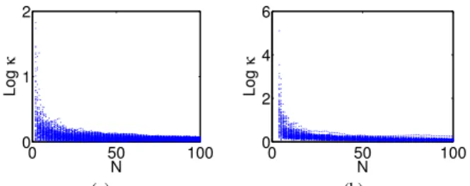
In Fig.1, we plot the logarithm of the condition number κ(R) of random realizations of R as N → ∞ for M = 2 and M = 4. It converges to 0 (i.e. the condition number converges to 1) for large N . As R converges to a multiple of identity, no inversion is needed when N → ∞. We just
0 50 100 0 1 2 N Log κ (a) 0 50 100 0 2 4 6 N Log κ (b)
Fig. 1. Convergence of the conditioning of a 1D SR problem
with respect to the number of images. (a) 80 realizations of the experiment with M = 2. (b) 80 realizations of the exper-iment with M= 4. 20 40 60 80 100 120 0 100 200 300 (a) 0 100 200 0 0.5 1 1.5 N e (b)
Fig. 2. Convergence of the estimatoru˜N. (a) Reference
sig-nal. (b) Reconstruction errors (light blue) for M=3 with pre-dicted convergence speed in red. In dark blue is the mean of the error for each N value (hidden under the prediction).
need to apply a normalized version of the adjoint operator of A to w. This operation gives the mean of back-shifted zero-padded LR images. We call ST the operation of up-sampling by zero-padding by a factor M . We have:
˜ uN = 1 N X i=1,N T−1 i S T wi−−−−→ N →∞ u (2)
The central limit theorem foru˜N gives a convergence speed
of √1
N for the L
2norm error of this estimator. In Fig.2, we
generate several SR experiments with the same reference sig-nal (line extracted from a natural image). We then plot the relative reconstruction error of the estimatoru˜N from
equa-tion (2) overlaid with the expected convergence speed. We showed in this part that, with a large number of im-age, a direct inversion is possible with a high probability. To achieve this result, we did not make any assumption on the HR image. It leads to an intuitive take on super-resolution: it is very interesting to take more images than the critical case to try to avoid regularization in the inversion process.
4. PERFECT INTERPOLATION IN A ROTATION-TRANSLATION SET UP
In this part, we extend the result on the critical number of images for perfect interpolation to motions composed of ro-tations and translations. We consequently write the transfor-mation of the LR images as a composition of rotations and
translations. We will consider the finite discrete case : A: (CM L×ML) → (CL×L)N
u→ (SRiTiu)i=1,N
Here, the Ti and Ri are the translations and rotations by
Shannon interpolation. A is a linear map on the vector space of discrete images. Thus, perfect recovery is possible if N≥ M2and A is full rank.
We now show that N ≥ M2is a sufficient condition under a
hypothesis on the transformations. Let us name the following sampling grids: Γhr = [1, M L]2 ⊂ Z2 andΓ = M.[1, L]2.
Γc
is the complement ofΓ in Γhr
, i.e. the support of images in the kernel of S. We write ri the rotation on the
coordi-nates for LR image i and ti the value of its translation. The
following theorem states a sufficient condition for A to be invertible: none of the displacement coordinates between two different transform of two points ofΓcshould be an integer.
Theorem 4.1. If N ≥ M2and∀p i, pj∈ Γc,1 ≤ k1< k2≤ N,||r−1 k1 pi−r −1 k2pj+(tk1−tk2) mod 1||0= 2 , A is injective.
Proof. We show by induction over N that adding a LR image decreased the dimension of the kernel of the function A by a factor L2. We demonstrated the necessary lemmas in the appendix for clarity purpose. Let:
An: (CM L×ML) → (CL×L)
u→ SRnTnu
We prove :∀1 < n ≤ M2, dim∩
k=1,nkerAk = (M2−n)L2
For n= 2: let pi∈ Γc. Let vi= 1pi. Let ui= T1−1R−11 vi.
We have Svi= 0. Consequently A1ui= 0 and ui ∈ kerA1.
We just defined (M2 − 1)L2 independent ui generating
kerA1: span(ui)i=1,(M2−1)L2 = kerA1. Similarly we
construct span(u′
i)i=1,(M2−1)L2 = kerA2. We
calcu-late the dimension of the intersection with Lemma A.2 (kerA1+ kerA2= CM L×ML):
dim(kerA1∩ kerA2) =
dim(kerA1) + dim(kerA2) − dim(kerA1+ kerA2)
= 2(M2− 1)L2− dim(kerA
1+ kerA2)
= (M2− 2)L2
Let n >2. Let us suppose that dim ∩k=1,nkerAk= (M2−
n)L2. We use Lemma A.3: (∩
k=1,nkerAk) + kerAn+1 =
CM L×ML. By using the same dimensions relation as for n=
2, we get the result.
The hypothesis on the transformation is not a necessary condition. In the proof, we imposed the invertibility in both spatial directions, which is stronger than necessary (e.g. the case of regular sampling is excluded but is already known), but the space of excluded motion parameters has measure 0.
5. LOCAL CONDITIONING IN A ROTATION-TRANSLATION SET UP
The fusion of rotated-translated grids is a sampling grid which is generally not periodic. We expect local variations of the spatial distribution of samples leading to a spatial variability in the noise generated by the inversion of the system. In this section, we show that we can predict this conditioning when rotations are small (which would be a reasonable hypothesis for a hand held camera), and use this prediction to regularize adaptively with respect to local conditioning.
We study the conditioning in the critical case N = M2
where the problem is invertible (from the previous section). We compare the reconstruction noise nrecof the system and
the reconstruction noise of a pure translational model at each location. When LR images are contaminated by a noise n, the reconstruction noise is nrec= A−1n.
We calculate the power of this noise locally. We restrict the image space of the application A−1to one LR pixel in the
HR image space to study its local behavior. Let x0= [x0, y0].
Let x ∈ [x0, x0+ M − 1] × [y0, y0+ M − 1] = D ⊂ Z2.
Let 1xbe the indicator function x∈ D in the HR image. We
now consider the mapping: A−1
x0 : E = A(span((1x)x∈D) → F = span((1x)x∈D)
w→ A−1w
We call local conditioning at position x0, the conditioning
of A−1
x0. This conditioning is the ratio of the bounds of the
quantity (greatest and smallest singular values): ||A−1
x0w||, ||w|| = 1
We can calculate equivalently the bounds of||Ax0u||, ||u|| =
1. Let u =P bk1xk∈ F with ||u|| = 1. We have :
||Ax0u|| 2= ||X bkA1xk||2 = X k1,k2 ¯bk1bk2(1xk1) H AHA1xk2 = X k1,k2 ¯bk1bk2 X i=1,N X y∈Γ
sincd(y − τi,k1)sincd(y − τi,k2)
where sincd is the finite discrete Shannon interpolator and τi,k = ri(xk− ti). Because sincd is differentiable, we can
use the mean value theorem to compare this expression to a pure translational one and obtain an expression of the form:
|||Ax0u||
2− ||Atr x0u||
2| ≤ K||t − ttr||
where t = (τi,k)i,k is the set of translations induced by the
motion, ttris t averaged over the HR pixel (over index k) and Atr
x0 is the translational SR operator associated with t tr
and K is a constant which does not depend on x0. Thus, for small
rotations, the noise of the system will behave as in a pure translational case. Experiments showed that for rotations in
a small range (-5,+5 degrees), we can use κ(x0) = cond(R)
as a local conditioning measure, with R defined as in section 3 with the translations ttr. This measure can be calculated a priori because it only depends on motion parameters, M and the size of the image.
We propose a local total variation regularization scheme where our local conditioning measure defines weights for the TV term. We minimize the function:
J2(˜u) = J(˜u) + H(˜u)
H(˜u) = Z
α.|∇˜u|
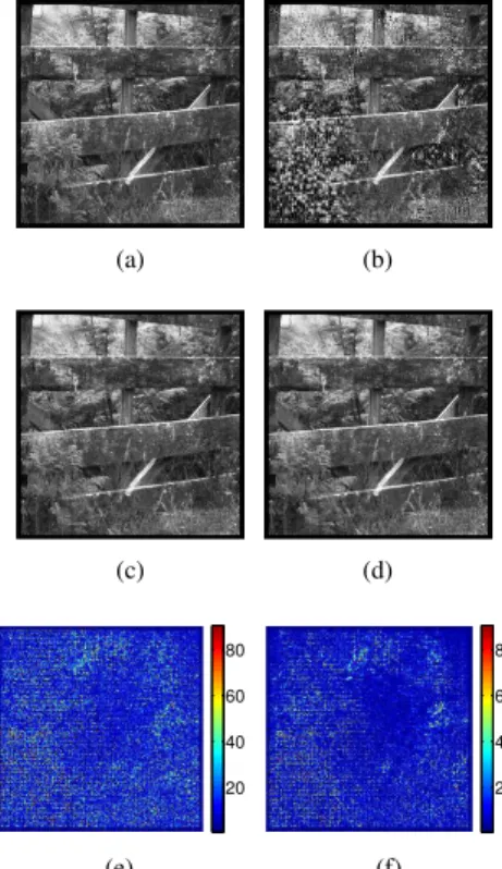
where α(x) = λlog(κ(x)). The choice of the logarithm was driven by experiments where other increasing functions were tested (identity, square-root). λ is the regularization param-eter. Conventional TV regularization is achieved by taking α(x) = λ. The selection of an optimal λ is an issue which is not adressed here. In the following experiments, we choose the λ achieving the best reconstruction in the L2 sense for global TV regularization and local TV regularization. We show in Fig.3 how we predict local conditioning. We gen-erate 9 noisy LR images from a240 × 240 HR image (SR with M = 3, rotations between −5 and 5 degrees, transla-tion distributed in[0, M ]2) and perform the inversion of the
system (1) without regularization. The amplitude of the re-construction noise and the corresponding prediction of the lo-cal conditioning show a good spatial correlation. The fusion of the points of the 9 grids also illustrates the spatially vary-ing nature of the samplvary-ing density. In Fig.4, SR interpola-tion without regularizainterpola-tion, with a global TV regularizainterpola-tion or with our local regularization scheme are compared. In Fig.4, reconstruction without regularization is perfect in well con-ditioned areas. Global TV regularization does not take into account the spatial variations of the sampling density. Thus, the regularization parameter λ is a trade-off. A large value for λ would be needed to fill parts where holes are big (because of the bad local conditioning of the data fit part) and a small one for well conditioned areas. Consequently, the resulting image is smoothed excessively in well conditioned areas and not enough in badly conditioned areas. With local regulariza-tion, smoothing occurs only in badly conditioned areas. Dif-ferences are mostly noticeable in the images of the residuals (Fig.4 (e) (f) displayed at the same scale).
6. CONCLUSION
We have studied super-resolution interpolation under several aspects. We showed that the conditioning depends on the number of images: if many LR images are available, the like-lihood of a bad conditioning decreases. Avoiding regular-ization accordingly would lead to SR interpolation without hypothesis on the nature of the image. For more complex motions (rotations + translations), we showed that the critical
(a) (b) 20 40 60 80 (c) 20 40 60 80 (d)
Fig. 3. Local conditioning of the SR problem. (a) Zoom on
the fusion of the 9 LR grids (40 × 40 pixels upper left corner). (b) one LR image. (c) Amplitude of the reconstruction error normalized by the input noise variance. (d) Local condition-ing2pκ(x). (a) (b) (c) (d) 20 40 60 80 (e) 20 40 60 80 (f)
Fig. 4. Local TV regularization for critical SR. (a) HR image.
(b) Reconstruction without regularization, PSNR=11.38db. (c) Reconstruction with best global TV regularization, PSNR=27.11db. (d) Reconstruction with our local regular-ization, PSNR=29.23db. (e) Reconstruction error with best global TV regularization. (f) Reconstruction error with our local regularization.
condition on the number of images still holds and is suffi-cient almost surely. To fill the gap between well conditioned invertible and ill-posed SR, we propose a way to regularize locally the reconstruction problem when camera rotation is small. With these developments, this paper completes the available set of SR interpolation methods to the well posed and badly conditioned invertible cases.
7. REFERENCES
[1] Jing Tian and Kai-Kuang Ma, “A survey on super-resolution imaging,” Signal, Image and Video
Process-ing, pp. 1–14, Feb. 2011.
[2] Sina Farsiu, Dirk Robinson, Michael Elad, and Pey-man Milanfar, “Advances and challenges in super-resolution,” Int. J. Imaging Syst. Technol., vol. 14, no. 2, pp. 47–57, 2004.
[3] Kim-Hui Yap, Yu He, Yushuang Tian, and Lap-Pui Chau, “A Nonlinear-Norm Approach for Joint Image Registration and Super-Resolution,” Signal Processing
Letters, IEEE, vol. 16, no. 11, pp. 981–984, Nov. 2009. [4] M. D. Robinson, C. A. Toth, J. Y. Lo, and S. Farsiu,
“Efficient Fourier-Wavelet Super-Resolution,” Image Processing, IEEE Transactions on, vol. 19, no. 10, pp. 2669–2681, Oct. 2010.
[5] R. C. Hardie, K. J. Barnard, and E. E. Armstrong, “Joint MAP registration and high-resolution image estimation using a sequence of undersampled images,” Image
Pro-cessing, IEEE Transactions on, vol. 6, no. 12, pp. 1621– 1633, Dec. 1997.
[6] Yann Gousseau and Jean-Michel Morel, “Are Natural Images of Bounded Variation?,” SIAM J. on
Mathemat-ical Analysis, vol. 33, pp. 634+, 2001.
[7] K. Gr¨ochenig and T. Strohmer, “Numerical and theo-retical aspects of nonuniform sampling of band-limited images,” in Nonuniform sampling : Theory and
Prac-tice, Inf. Technol. Transm. Process. Storage, pp. 283– 324. Kluwer/Plenum, New York, 2001.
[8] Gabriele Facciolo, Andres Almansa, Jean-Francois Au-jol, and Vicent Caselles, “Irregular to Regular Sampling, Denoising, and Deconvolution,” Multiscale Modeling &
Simulation, vol. 7, no. 4, pp. 1574+, 2009.
[9] A. Papoulis, “Generalized sampling expansion,”
Cir-cuits and Systems, IEEE Transactions on, vol. 24, no. 11, pp. 652–654, Nov. 1977.
[10] Simon Baker and Takeo Kanade, “Limits on Super-Resolution and How to Break Them,” IEEE
Transac-tions on Pattern Analysis and Machine Intelligence, vol. 24, no. 9, pp. 1167–1183, 2002.
[11] D. Robinson and P. Milanfar, “Statistical performance analysis of super-resolution,” Image Processing, IEEE
Transactions on, vol. 15, no. 6, pp. 1413–1428, June 2006.
[12] Fr´ed´eric Champagnat, Guy Le Besnerais, and Caro-line Kulcs´ar, “Statistical performance modeling for su-perresolution: a discrete data-continuous reconstruction framework,” J. Opt. Soc. Am. A, vol. 26, no. 7, pp. 1730– 1746, July 2009.
A. APPENDIX
Lemma A.1. For1 ≤ i ≤ N , let ui ∈ Cn×n, ui(r, s) =
xr
iyis, we call ui2D Vandermonde vectors with seed[xi, yi]. If
∀1 ≤ i < j ≤ N, xi 6= xj, yi 6= yj, dim(span(ui)i=1,N) =
min(N, n2).
Proof. We show that the uiare linearly independent if N ≤
n2. Let us supposeP λiui = 0. Let ui(s) = Xiysi with
Xi = (xri)r.∀s,P λiui(s) =P λiXiysi = 0. The Xiform
an independent family of 1D Vandermonde vectors. It implies ∀s,P λiyis= 0 which we rewriteP λiYi= 0, but the Yiare
also independent. Consequently, λi= 0.
Lemma A.2. If ∀pi, pj ∈ Γc,||r1−1pi − r2−1pj + (t1 −
t2) mod 1||0= 2, kerA1+ kerA2= CM L×ML.
Proof. We can construct a basis of kerA1and kerA2by
tak-ing the inverse transformations of the indicator functions of the pixels zeroed by the subsampling. In the Fourier domain, these bases are:
ˆ ui(ω) = e−j<ω,r −1 1 pi+t1>,uˆ′ i(ω) = e−j<ω,r −1 2 pi+t2>
which are 2D Vandermonde vectors with seed[e−j<ex,r−1k pi+tk>,
e−j<ey,rk−1pi+tk>]. We use Lemma A.1: kerA
1+ kerA2 =
span((ˆui), (ˆu′i)) = CM L×ML(the seeds are all different
be-cause∀pi, pj,||r−11 pi− r2p−1j + t1− t2mod1||0= 2). Lemma A.3. Let N < M2.If∀pi, pj ∈ Γc,1 ≤ k1 < k2 ≤
N,||r−1 k1pi− r
−1
k2pj+ (tk1− tk2) mod 1||0= 2 and
dim(∩k=1,nkerAk) = (M2− n)L2 then∩k=1,nkerAk +
kerAn+1= CM L×ML.
Proof. Let (ei) be a basis of ∩k=1,nkerAk of size (M2−
n)L2. In the basis(u j)j=1,nof kerA1,: ei = X αi,juj Let u′
i a basis of kerAn. With the hypothesis, any linear
combination of ei, u′iis a linear combination of independent
Vandermonde vectors. Therefore, dim(span((ˆei), (ˆu′i))) =
min((M L)2,(M2 − n)L2 + (M2 − 1)L2) = (M L)2.
Thus, we have∩k=1,nkerAk+ kerA2= span((ˆei), (ˆu′i)) =