A Parallel Supercomputer Implementation of a Biological
Inspired Neural Network and its use for Pattern
Recognition
Vincent de Ladurantaye, Jean Lavoie, Jocelyn Bergeron, Maxime Parenteau, Huizhong Lu, Ramin Pichevar, Jean Rouat1
NECOTIS, GEGI, Univ. de Sherbrooke Qu´e., CANADA. http://www.gel.usherbrooke.ca/necotis
Abstract. A parallel implementation of a large spiking neural network is proposed and evaluated. The neural network implements the binding by synchrony process using the Oscillatory Dynamic Link Matcher (ODLM). Scalability, speed and performance are compared for 2 implementations: Message Passing Interface (MPI) and Compute Unified Device Architecture (CUDA) running on clusters of multicore supercomputers and NVIDIA graphical processing units respectively. A global spiking list that represents at each instant the state of the neural network is described. This list indexes each neuron that fires during the current simulation time so that the influence of their spikes are simultaneously processed on all computing units. Our implementation shows a good scalability for very large networks. A complex and large spiking neural network has been implemented in parallel with success, thus paving the road towards real-life applications based on networks of spiking neurons. MPI offers a better scalability than CUDA, while the CUDA implementation on a GeForce GTX 285 gives the best cost to performance ratio. When running the neural network on the GTX 285, the processing speed is comparable to the MPI implementation on RQCHP’s Mammouth parallel with 64 notes (128 cores).
1. Introduction
One of the greatest engineering challenges faced in the 21st century is to understand and reproduce the functioning of the brain. Binding by synchrony is an important function that explains a great number of behaviors like perception of objects and polysensoriality [1, 2]. With the arrival of parallel computing, simulation of large artificial neural networks is becoming feasible. It is now realistic to implement the binding function for use in artificial intelligence or in the area of computational neuroscience. The challenge behind such work is the great number of interconnections making each unit dependent on many others and thus limiting data independence, which is crucial for effective parallel computing. A parallel implementation of the binding function with spiking neural network (SNN), as proposed by Pichevar et al. [3], is described. Also, the scalability for large networks and performance comparison between multi-core computers (MPI) and graphical processing units (GPUs : CUDA) implementations is evaluated.
1
CUDA conception and experiments by V. de Ladurantaye; MPI experiments by V. de Ladurantaye and M. Parenteau; MPI architecture conceived or realized by J. Lavoie, J. Bergeron, H. Lu, M. Parenteau, R. Pichevar and J. Rouat; V. de Ladurantaye and J. Rouat are primary authors.
2. Parallel Implementations of Spiking Neural Networks
Biologically accurate models of neurons like the Hodgkin-Huxley model [4] require the integration of 4 non-linear equations which is very computationally intensive. On the other hand, the integrate and fire model [5] is less biologically realistic but requires a single linear equation. Izhikevich proposed a 2-equation model that is a good compromise between speed and biological accuracy [6]. To use spiking neurons on parallel supercomputers, SNN simulators such as NEURON, PGENESIS and NEST have been developed [7]. Those simulators are based on MPI and have been reported to have a good scalability for large network simulations [8]. However, with the recent arrival of GPU technology, much interest is now on graphical processor implementations. The Izhikevich [9, 10, 11] and the integrate and fire models [12] have been ported to GPU using the CUDA plateform. Pallipuram et al. [13] have compared implementations on different GPU programming models and architectures. Also, Han and Tarek have proposed a mixed architecture using an MPI implementation running on clusters of GPUs [14]. These implementations are usually done on networks of relatively simple complexity, with the maximum number of synaptic connections never exceeding one million. In this work, we implement a large scale SNN using integrate-and-fire neurons in a network which is almost fully connected with a number of synaptic connexions as high as several billions. Furthermore, we simulate and use the binding function in an image comparison task. To our knowledge there is no other parallel implementation of image processing applications based on the binding occurring in the brain.
3. Model Description and application in image comparison 3.1. Neuronal model
The implemented Oscillatory Dynamic Link Matcher (ODLM) network [3] uses leaky integrate-and-fire neurons. The membrane potential v(t) of an isolated neuron evolves through time according to:
v(t) = I0 C(1 − e
−t
τ) (1)
When v(t) becomes greater or equal to a fixed threshold θ, at time tspike, then the neuron emits a spike δ(t − tspike) and v(t) is reset to 0. τ is a time constant that controls the amount of leaky current and thus, the speed. C is a constant and I0is a constant input current.
3.2. The architecture of the Oscillatory Dynamic Link Matcher for image comparisons
For the image comparison task at hand, the SNN comprises two layers with local connectivity within each layer and full connectivity between different layers. A neural layer is attributed to each image and each pixel is associated with a spiking neuron as illustrated in figure 1. Synaptic connexions are symmetrical and bidirectionnal (Fig. 1). For a given neuron (i, j), the state equation of the system is given by dvi,j dt = − 1 τvi,j(t) + 1 CI0+ Si,j(t) (2) with Si,j(t) = X k,m∈Next(i,j)
{wexti,j;k,mδ(t − tspikek,m)} +
X
k,m∈Nint(i,j)
{wi,j;k,mint δ(t − tspikek,m)} − ηG(t) (3)
Si,j(t) is the total contribution that a neuron (i, j) receives from all neurons (k, m) it is connected to; whether they are on the same layer (int) or on a different layer (ext). Next(i, j) and Nint(i, j) are the sets of firing neurons (k, m) to which neuron (i, j) is connected. G(t) is a global inhibitor that regulates the neural network activity. η is a constant that controls the influence of the global inhibitor.
The connecting weights have the respective expressions wi,j;k,mint = w
int max
Card{Nint(i, j)}e
−λ|pi,j−pk,m| inside a layer (4)
wi,j;k,mext = w ext
maxf (SegCompactness, SegAveragedgrey)
Card{Next(i, j)} e
−λ|pi,j−pk,m| between layers (5)
In this simple application pk,m and pi,j are pixel values associated respectively to neurons (k, m) and (i, j). Card{Nint(i, j)} and Card{Next(i, j)} are normalization factors corresponding to the number of active neurons (k, m) that are connected to neurons (i, j) whether they are inside the same layer (int) or in a different layer (ext). Two processing phases are defined: the segmentation and the matching. During the segmentation phase, the connections between layers are not activated (wexti,j;k,m= 0). Once the images have been independently segmented, the two layers are connected with wi,j;k,mext derived from equation 5, thus creating the matching phase. f (SegCompactness, SegAveragedgrey) is a weighting function that modulates the external weight connections depending on the averaged grey level and of the compactness (segment squared perimeter over the surface) of the segment to which neuron (i, j) belongs. 3.3. Binding by synchronization and the image comparison experiment
Two images shown in figure 2(a) are respectively presented to each layer. Neurons with strong connections tend to synchronize with each other, thus forming segments of synchronized neurons representing a similar part of the image (fig. 2(b)). Instead of using image features like contours, orientations, etc., pixel grey values are inputs to the computation of the connexion weights (equations 4, 5). This is not an ideal situation as recognition scores are lower with pixel values than with image features. However, this naive input setting yields a much more complex network with the number of connexions growing exponentially with the size of the images. With two 200p x 200p images, the network comprises 80 000 neurons with more than 1.6 x 10⁹ connections. In this work our main interest is in fact the implementation of a complex network. At this stage, we are not interested in simplification and reduction of the network size. The matching phase begins once the segmentation is completed. It also uses the information from the segments to connect neurons between the two layers according to equation 5. Neurons within segments with similar grey scale values and compactness are strongly connected and thus the matching phase tends to synchronize similar parts of the two images as shown in figure 2(c).
Figure 1. Architecture of the 2 layer neural network: neurons are locally coupled inside a layer and fully connected between layers. G is a global regulation unit that reduces the activity of the neural network (with inhibition) when the NN is too active.
4. Network parallelization
4.1. Distribution on processing units and event-driven processing
Neurons are uniformly distributed on different computing units and since we have a great number of neurons, this allows for a good level of scalability. However, the problem we face is that neurons are not independent of each other. A neuron can be affected by a spike coming from any processing unit at any
(a) (b) (c)
Figure 2. (a) Images used as input. (b) Segments formed after the segmentation phase. The color encodes the time at which neurons emit spikes. (c) Results of the matching phase between the two images.
time. In a network that is very strongly connected, this yields a data dependency that is very problematic for massively parallel architectures. An event-driven time management is therefore implemented as described in [7] to avoid calculating uneventful time steps between neuron spikes. By finding the neuron with the highest membrane potential in the network, one can advance the time to the moment at which the neuron will fire.
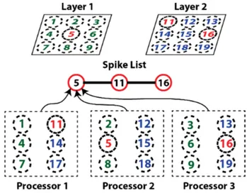
Since neurons are distributed on different processing units, they do not have access to neurons spiking on a different thread (threads can be associated to a different processing units). Thus, a global mechanism must be used that regroups the spiking neurons in a list that is available to all computing units. This is illustrated in figure 3. Individual neurons are then able to independently iterate through that list and react accordingly if they are connected to a neuron that spikes.
Figure 3. Example of parallel distribution of neurons and interaction with the global spike list. Neurons from layer 1 and 2 are distributed evenly on the 3 processors. This example shows the network in a state where there are 3 neurons spiking simultaneously (in red). All spiking neurons are put into the spiking list which is available to all processors. All processors iterate in parallel through the spiking list and process the spikes on their local neurons.
4.2. Differences between parallel and serial implementations
Memory management is different in the serial (conventional) and the parallel implementations. In the sequential version, all synaptic weights are stored in memory. However, for the parallel version, because of limited local memory size, synaptic weights for all neurons cannot be stored. Instead, the synaptic weight between two neurons is computed (with equations 4 and 5) when the receiving neuron fetches the spiking neuron information in the global spiking list. As such, the spiking list contains the ID of the spiking neurons along with the information needed by other neurons to compute the synaptic weight linking them.
5. Platform implementation
Implementation of the model was realized on two different architectures: Message Passing Interface (MPI) and Compute Unified Device Architecture (CUDA). The MPI implementation is used for platforms such as multi-core PCs or clustered computers whereas CUDA is for Nvidia’s GPUs. Each architecture brings a different level of parallelization, but also different constraints. This is described in the following subsections.
5.1. MPI Implementation
Computations are distributed as processes which can be scattered on different computing nodes. Each node is independent and has its own local memory. MPI is an interface that allows messages to be passed between the different processes to exchange data and synchronize computation. However, communications and data exchange are costly and need to be kept to a minimum by trying to constrain dependent data to a single process. Once computations run within the scope of a single process, it is equivalent as doing computation on a CPU.
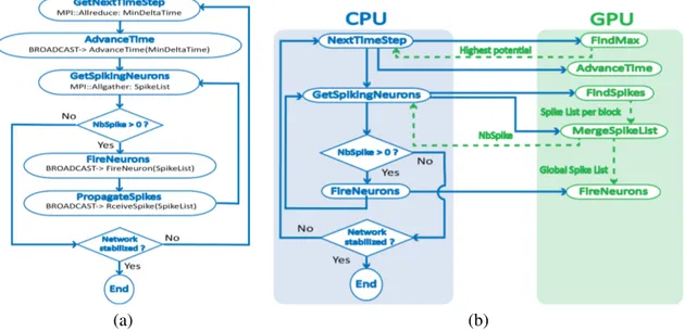
For the neural network implementation, each process is in charge of a group of neurons that resides in local memory for the duration of the simulation. Neurons are distributed on available processes with no particular order as the connections are too numerous to restrict communications within individual nodes. MPI collective operations are used to gather data distributed on the different processes, and general broadcast messages are used to instruct the processes of the computations they need to do on their neurons. The general program flow of the MPI implementation is shown in figure 4 (a).
(a) (b)
Figure 4. Execution flow of the program for both MPI (a) and CUDA (b) implementations. Both implementations follow the same general algorithm. It starts by finding the neuron with the highest potential. Then simulation time is advanced to when it fires. A list of spiking neurons is collected and spikes are finally computed. This is done iteratively untill there are no more spikes left. This iterative process represents one simulation cycle. Once a cycle is done, network stability is verified (the network is stable when the spike patterns are the same over multiple cycles).
Each process finds the neuron with the highest potential within its assigned neurons and computes the time needed for it to spike. Using the collective operation MPI AllReduce, which allows to find the minimal value of a variable distributed among all processes, the smallest time (MinDeltaTime) is isolated. It is then broadcasted in the system within a AdvanceTime message, that instructs the processes to advance the simulation time on their neurons. The global spiking list is assembled using the collective
operation MPI Allgather, which allows the gathering of data that is distributed on all processes. The FireNeurons and PropagateSpikes messages are then broadcasted with the spike list, instructing the processes to check if they are responsible for neurons affected by the spike list. The FireNeurons message instructs the processes to handle the computations of the spiking neurons themselves, that is resetting their internal potential. The PropagateSpikes message on the other hand, handles the computations on the neurons receiving a spike from a neuron in the spiking list.
5.2. Cuda Implementation
Computations are launched from the PC as kernels running on the GPU. A kernel consists of CUDA code that is distributed as blocks on the GPU. A block is a group of threads running on the graphic card processors, and collaborating together on the same data. Nvidia’s GPUs have global memory, which is available to all threads, and also local memory which is very fast and shared within a block. Local memory is very limited, and thus, CUDA code needs to be designed to maximize its use, and also to minimize exchanges with the PC which are very costly.
For the neural network implementation, the CPU controls the flow of the program as shown in figure 4 (b). When the neurons need to be manipulated, a CUDA kernel is called to launch the calculations on the GPU. A different kernel is used for each specific task because local resources usage changes depending on the computations. Kernels are individually optimized to use available resources as efficiently as possible, so the number of neurons handled per block varies depending on the kernel. Typically, each kernel is separated in blocks handling several hundreds of neurons at a time. All neuron data is kept in global memory. Each time a kernel is called, it loads the data of its assigned neurons in local memory, executes the required computations and returns the result in global memory.
The FindMax and AdvanceTime kernels find the next neuron to spike and advance the simulation time respectively. The highest neuron potential is sent to the CPU so it can keep track of the simulation time. The FindSpike kernel finds the neurons that have a potential above the firing threshold and creates a spike list for each CUDA block. Since blocks do not share memory, the MergeSpikeList kernel is used to merge all the spike list and create a single list. The total number of spiking neuron is sent to the CPU to determine which kernel needs to be launched next. If the list is not empty, the FireNeurons kernel is launched to compute the impact of the spiking neuron on the network. The FireNeurons kernel works, as mentioned before, by making all neurons in the network iterate through the global spiking list, and by performing the appropriate computations if a local neuron is affected by a spike.
6. Results and Discussion 6.1. Experimental setup
The MPI implementation was tested on a dual quad core (AMD Opteron 2.2Ghz), and on RQCHP’s Mammouth MP (2 CPUs/nodes (3.6GHz), 8GB/nodes, switch-infiniband). The CUDA implementation was tested on a Tesla C870 and a GeForce GTX285 from Nvidia.
For each implementation, the same 2 input images (Fig. 2) are presented to the neural network. Various network sizes are obtained by modifying the image resolutions. As the initialization values are randomized, the total number of iterations can vary between simulations. To ensure equivalent workload, instead of waiting for the network to stabilize, the number of iterations is arbitrarily fixed : 250 iterations for the segmentation of each image and 500 matching iterations for a total of 1000 cycles. To validate the different implementations, an image comparison benchmark is run and we verify that results are the same for all platforms.
6.2. Results
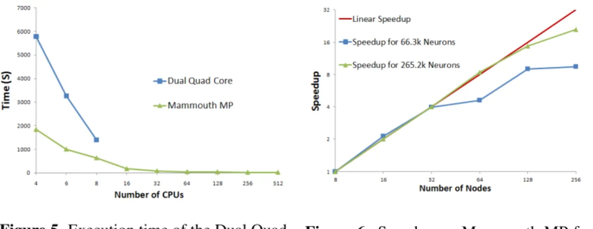
Table 1 gives the simulation times for different network sizes on different platforms. As can be seen, the MPI implementation running on the dual quad core is slower than the sequential implementation of the model. For Mammouth MP, performance is similar to the sequential version using only 2 nodes, which is
4 CPUs. As shown in figure 5, the execution time is greatly reduced as the number of CPUs is increased. Therefore, more than 8 CPUs on the dual quad core,would be faster than the sequential version.
Platform Network size in nb. of neurons 4.1k 16.6k 66.3k 265.2k
Sequential CPU 3 59 -
-Dual Quad Core 5 74 1394 41383
Mammouth MP (2 Nodes) 4 60 1838
-Mammouth MP (32 Nodes) 2 4 43 684
Mammouth MP (64 Nodes) 3 4 37 327
Tesla C870 2 8 75 2345
GeForce GTX 285 2 4 19 467
Table 1. Execution time in seconds for the simulation of different network sizes on different platforms. Sequential CPU simulations for network bigger than 16.6k neurons were not run because the memory requirement would be too high.
Figure 6 shows the scalability of our MPI implementation on Mammouth MP from 8 nodes up to 256 nodes. The speedup scales well with the number of processing nodes. The bigger the neural network, the better the speedup. When the network size gets relatively small (thousands of neurons for each processing core), the speedup function is no longer linear (Fig. 6).
Figure 5. Execution time of the Dual Quad Core versus Mammouth MP
Figure 6. Speedup on Mammouth MP for the number of node used
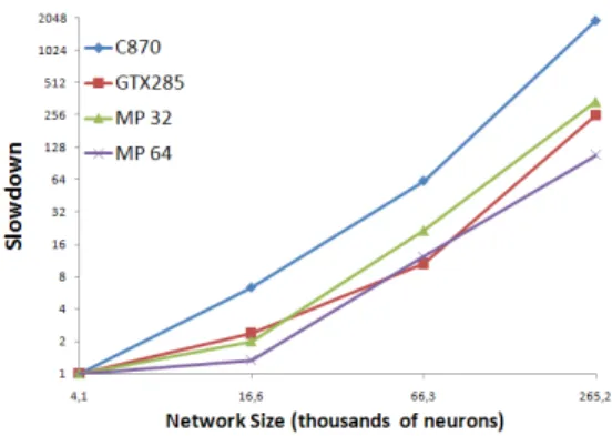
As for the CUDA implementation, (Table 1) the C870 is much slower than the GTX 285. This is mainly explained by the higher bandwidth on the GTX 285 rather than the greater number of processing units. Neurons are loaded in memory much faster, an operation that has to be done at each kernel execution. With 64 nodes, Mammouth Parallel (MP) has roughly equivalent performance to the GTX 285. It is important to note however, that the MPI implementation scales better with increasing network size than the CUDA implementation. This is shown more explicitly in figure 7, where a slowdown is observed when increasing the network size. The slope of the graph is greater for both GPUs than for MP. In fact, the CUDA implementation has to reload the neuron’s data from global memory for every kernel execution while on the MPI implementation, the neuron’s data never moves from the process to which they are initially assigned. The bigger the network, the more data transfer have to be done in the CUDA implementation whereas there is simply no transfer needed for MPI.
7. Conclusion
Parallel implementations of a strongly connected large scale spiking neural network were presented for both MPI and CUDA architectures. On Mammouth MP, scaling of the MPI implementation with the number of available cores was shown to be very good, following an almost linear speedup with very
Figure 7. Slowdown observed on different platforms with increasing network size
large neural networks. The CUDA implementation presented similar performance using a GTX 285, compared with Mamouth MP with 64 nodes. However, the MPI version was shown to scale better with network size than the CUDA version.
Considering the of cost to performance ratio for parallel implementation of spiking neural networks, GPUs show the best trade off. Although, the current CUDA implementation should be redesigned to avoid reloading the neurons’ data, which doesn’t necessarily change from a kernel to the other. Local data persisting through kernel execution would be a great feature for this application (though it may not be technically feasible).
For real image processing applications, it is not necessary to let the network iterate as much as in the presented experiments. Also, suitable initial conditions accelerate the convergence speed of the neural network. So care should be taken as not to extrapolate the current processing speed to real applications. The goal of this paper was to demonstrate the parallel implementation effectiveness of a spiking neural network implementing the binding operation between two layers of neurons. The findings can be generalized to any application other than image processing as long as the topology of the neural network is comparable (local connections inside layers and full connections between layers) and that weights between neurons can be computed online.
Acknowledgment
CRSNG, Univ. de Sherbrooke, OPAL-RT for funding the research. Vincent Tremblay Boucher, Julien Beaumier- ´Ethier, Alexandre Provencher and Jonathan Verdier for CUDA programming. Many thanks to Sean Wood for correcting English.
References
[1] Milner P 1974 Psychological Review 81 521–535 [2] Molotchnikoff S and Rouat J 2011 Frontiers in Bioscience
[3] Pichevar R, Rouat J and Tai L 2006 Neurocomputing 69 1837–1849 [4] Hodgkin A L and Huxley A F 1952 J Physiol 117 500–544 [5] Gerstner W 1998 Pulsed Neural Networks (The MIT Press)
[6] Izhikevich E 2003 IEEE Transactions on Neural Networks 14 1569–1572 [7] Brette R and et al 2007 Journal of Computational Neuroscience 23 349–398
[8] Plesser H E, Eppler J M, Morrison A, Diesmann M and Gewaltig M-O 2007 Euro. Conf. on Parallel Processing 672–681 [9] Nageswaran J M, Dutt N, Krichmar J L, Nicolau A and Veidenbaum A 2009 IJCNN 2009 3201–3208
[10] Fidjeland A and Shanahan M 2010 IJCNN 2010
[11] Yudanov D, Shaaban M, Melton R and Reznik L 2010 IJCNN 2010
[12] Nageswaran J, Dutt N, Wang Y and Delbrueck T 2009 2009 IEEE Int. Symp. on Circuits and Systems 1917 – 20 [13] Pallipuram V K, Bhuiyan M and Smith M C 2011 Journal of Supercomputing 1 – 46