Synoptic-Scale Atmospheric Circulation and Boreal Canada Summer Drought
Variability of the Past Three Centuries
MARTIN-PHILIPPE GIRARDIN*AND JACQUESC. TARDIF
Centre for Forest Interdisciplinary Research, University of Winnipeg, Winnipeg, Manitoba, Canada
MIKED. FLANNIGAN
Natural Resources Canada, Canadian Forest Service, Sault Sainte Marie, Ontario, Canada
YVESBERGERON
Groupe de Recherche en E´ cologie Forestière Inter-Universitaire, Université du Québec à Montréal, Montreal, Quebec, Canada
(Manuscript received 4 January 2005, in final form 30 September 2005) ABSTRACT
Five independent multicentury reconstructions of the July Canadian Drought Code and one reconstruc-tion of the mean July–August temperature were developed using a network of 120 well-replicated tree-ring chronologies covering the area of the eastern Boreal Plains to the eastern Boreal Shield of Canada. The reconstructions were performed using 54 time-varying reconstruction submodels that explained up to 50% of the regional drought variance during the period of 1919–84. Spatial correlation fields on the six recon-structions revealed that the meridional component of the climate system from central to eastern Canada increased since the mid–nineteenth century. The most obvious change was observed in the decadal scale of variability. Using 500-hPa geopotential height and wind composites, this zonal to meridional transition was interpreted as a response to an amplification of long waves flowing over the eastern North Pacific into boreal Canada, from approximately 1851 to 1940. Composites with NOAA Extended Reconstructed SSTs indicated a coupling between the meridional component and tropical and North Pacific SST for a period covering at least the past 150 yr, supporting previous findings of a summertime global ocean–atmosphere– land surface coupling. This change in the global atmospheric circulation could be a key element toward understanding the observed temporal changes in the Canadian boreal forest fire regimes over the past 150 yr.
1. Introduction
Forest fires are responsible for the spatial and tem-poral variations in the forest mosaic of the boreal forest (Bourgeau-Chavez et al. 2000). Fire has been an inte-gral ecological process since the arrival of vegetation on the landscape. Weather and climate are important de-terminants of fire activity (Flannigan and Harrington
1988; Johnson 1992; Flannigan and Wotton 2001). In particular, the frequency of precipitation through the fire season rather than the amount of precipitation is a critical aspect of the weather in terms of fire activity. A low frequency of precipitation is associated with a high probability of a large burned area, and vice versa (Flan-nigan and Harrington 1988; Flan(Flan-nigan and Van Wagner 1991). Another key weather aspect is blocking ridges in the upper atmosphere. Most of the area burned in the boreal forest of Canada is attributed to large-blocking high pressure systems at the 500-hPa atmospheric pres-sure level that cause dry fuel conditions (Skinner et al. 1999, 2002; Flannigan and Wotton 2001). When high pressure systems begin to break down, convective ac-tivity leading to numerous lightning strikes occurs and this ignites forest fires (Nash and Johnson 1996).
Climate and the associated weather are always * Current affiliation: Natural Resources Canada, Canadian Forest
Service, Laurentian Forestry Centre, Quebec City, Quebec, Canada.
Corresponding author address: Martin-Philippe Girardin,
Cana-dian Forest Service, Laurentian Forestry Centre, 1055, rue du P.E.P.S., C.P. 10380, Stn. Sainte-Foy, Quebec City, QC G1V 4C7, Canada.
E-mail: [email protected]
© 2006 American Meteorological Society
changing because of a number of factors such as solar variability, changes in the chemical composition of the atmosphere, and volcanoes. Thus, with a dynamic cli-mate and the strong linkage between clicli-mate and forest fires, variations in historical observations of fire activity resulting from changes in the climate and weather are expected. Studies have suggested that the fire regime in the Canadian boreal forest changed after the end of the Little Ice Age (⬃1850). The age distributions of forest stands across large areas of the Canadian boreal forest, reconstructed from living trees, snags, and downed woody material, suggest that fire frequency and the area burned have significantly diminished since 1850 (Larsen 1996; Weir et al. 2000; Bergeron et al. 2001; Bergeron et al. 2004). The existence of a trend toward a more moist climate in eastern boreal Canada was further documented in studies of forest communities located in flood-prone environments (Tardif and Berg-eron 1997a; Tardif and BergBerg-eron 1999), which revealed an increase in the frequency and magnitude of spring water levels at ice breakup. This trend agrees with stud-ies made in the Canadian Plains. Salinity reconstruc-tions in Alberta revealed that past aridity severity (1300–1750 period) was generally greater than that re-corded during the instrumental period (Sauchyn et al. 2002). While drought was frequent in the twentieth cen-tury, it tended to be of short duration and was sepa-rated by periods of relatively high precipitation (Sauchyn et al. 2003). With respect to fire weather se-verity under a 2 ⫻ CO2 scenario, general circulation
model (GCM) simulations predict a trend toward a moister climate in the Boreal Shield, and a drier climate in the Great Plains (Flannigan and Wotton 2001). This agrees with other simulations suggesting more intense, more frequent, and longer lasting 500-hPa-blocking high pressure systems over western-central North America, resulting from ongoing increases in green-house gases (Meehl and Tebaldi 2004).
Because of the relationship between atmospheric cir-culation and area burned, it was hypothesized that his-torical changes in the boreal forest fire regime were attributed to changes in the circulation of air masses (Bergeron and Archambault 1993; Hofgaard et al. 1999) and sea surface temperatures (SSTs; Girardin et al. 2004a). Ocean and atmosphere summertime cou-plings over Canada have been addressed and recog-nized by many authors (Bonsal et al. 1993; Bonsal and Lawford 1999; Nigam et al. 1999; Barlow et al. 2001; Girardin et al. 2004a,b; Shabbar and Skinner 2004). Nevertheless, most climate studies are based on short-term data and can provide little or no information on past climate history and its influence on vegetation dy-namics. Therefore, this paper investigates the spatial
and temporal variations observed in summer drought severity during the last three centuries in the eastern Boreal Plains and Boreal Shield of Canada. The extent to which the variability in the proxy records reflects changes in atmospheric and oceanic circulation is also explored.
2. Data and methods
Six independent annually resolved climate recon-structions going back to the early 1700s that are repre-sentative of climate variability from the eastern Boreal Plains to the eastern Boreal Shield were developed from a dense network of 120 tree-ring chronologies. Five of these were reconstructions of the July Canadian Drought Code (CDC; Turner 1972; Girardin et al. 2004a). The sixth was a reconstruction of the mean Ju-ly–August temperature. The dynamics between drought variability and atmospheric and oceanic drivers was analyzed using the National Centers for Environ-mental Prediction–National Center for Atmospheric Research (NCEP–NCAR) reanalysis gridded instru-mental 500-hPa geopotential heights and vector winds (1948–84; Kalnay et al. 1996), and National Oceanic and Atmospheric Administration (NOAA) Extended Reconstructed Sea Surface Temperatures (ERSST; 1854–84 period; Smith and Reynolds 2003).
a. Study area
The study area covers the eastern Boreal Plains to the eastern Boreal Shield ecozones, and most of the boreal forest from western Manitoba to eastern Quebec (Fig. 1). The study area covers six climate regions (Fig. 1), with boundaries approximating actual ecoregions defined by the Ecological Stratification Working Group (1996). These climate regions are the Boreal Plains (BP), Lac Seul Upland and Lake of the Woods (LS), Lake Nipigon (LN), the west and east Abitibi Plains (APw and APe, respectively), and southern Laurentian (SL) (Fig. 1).
All six regions under study have a subhumid to hu-mid hu-midboreal ecoclimate (west–east gradient), marked by warm summers and cold, snowy winters ac-cording to the Ecological Stratification Working Group’s (1996) regional classification. In the BP and LS regions, the average annual temperature ranges be-tween⫺1.0° and 1.0°C, whereas eastern regions from LN to SL range between 1.0° and 1.5°C. The average summer temperature is similar across the six regions, approximately 14.0°C. The average winter tempera-tures are more variable, ranging from⫺16.0°C in the BP region to⫺11.0°C in the SL region. The average
annual precipitation ranges from 450 mm in the west to 1600 mm in the east. Most of the annual precipitation in the study area falls between the months of June and October (Environment Canada 2002).
b. Development of the tree-ring residual chronologies
In winter 2001, a survey of available ring-width mea-surement series was made for the construction of a tree-ring chronology network. Sixty-three datasets were gathered from the International Tree Ring Data Bank
(ITRDB) data library (Archambault and Bergeron 1992; Hofgaard et al. 1999; Tardif and Bergeron 1997b; Jardon et al. 2003; Girardin et al. 2004a; Girardin and Tardif 2005). In 2002 and 2003, sampling was conducted in Ontario to fill gaps within the network; 57 datasets were collected. Tree-rings were sampled and cross dated using standard techniques (Yamaguchi 1991; Gi-rardin and Tardif 2005) and were validated using the COFECHA program (Holmes 1983).
In total, 120 datasets of ring-width measurement se-ries from 13 species and extending back to at least 1866 FIG. 1. (a) Geographical distribution of the locations of the 120 residual tree-ring
chro-nologies used for the climate reconstructions (squares). The different shades delineated the six regions. Supplemental chronologies used in a spatiotemporal analysis of radial growth are shown with circles (refer to section 3g). (b) Geographical distribution of the locations of the meteorological stations used in the calculation of the regional climate variables. (c) Domain of the area under study. Six regions enclosed by the shaded areas were selected for the climate reconstruction: BP, LS, LN, APw, APe, and SL.
were gathered for dendroclimatic reconstruction (Fig. 1; appendix A). The major species were conifers of the genus Pinus (45% of all datasets), with the exception of the Quebec area in which the genus Picea represented 51% of all datasets. The species Thuja occidentalis L. also represented an important fraction of the datasets (15%). In general, the datasets were well replicated, with only 13% of them being composed of less than 30 measurement series (appendix A). At least 25 chro-nologies had high subsample signal strength for a pe-riod covering the late-eighteenth century to present.
The age-/size-related trend was removed from the tree-ring measurement series using a spline function giving a 50% frequency response of 60 yr (Cook and Peters 1981). Although this detrending procedure re-sulted in the loss of information relative to long-term climate changes, 99% of the variance contained in fre-quencies lower than 19 yr was preserved. This “flex-ible” smoothing was necessary because many of the tree-ring series were less than 100 yr in length. The biological persistence contained in the standardized measurement series was removed (autoregressive mod-eling) to eliminate variation not resulting from climate (Cook and Holmes 1986). Biweight robust means of the residual measurement series were computed to create the residual chronologies. All chronologies were con-structed using the ARSTAN program (Holmes 1999).
c. Development of the climate data
Analyses of the tree growth–climate relationships were conducted using regional mean monthly average CDC (a description follows) from Girardin et al. (2004b), mean monthly temperature from Vincent and Gullett (1999), and total monthly precipitation from Mekis and Hogg (1999). The MET program from the Dendrochronology Program Library (Holmes 1999) was used to estimate the missing data for each station and to combine the stations into regional variables. Monthly variables for each station were normalized to give each station the same weight in calculating the mean values for each month and year. (Refer to Fig. 1b for the distribution of stations and to appendix B for a list of stations.)
The CDC is a daily component of the Fire Weather Index System (Van Wagner 1987) that is used across Canada by fire management agencies to monitor forest fire danger. It is an indicator of summertime moisture in deep organic layers in boreal conifer stands (Van Wagner 1970) and correlates well with radial growth of numerous boreal tree species (Bergeron and Archam-bault 1993; Tardif and Bergeron 1997b; Girardin et al. 2004a; Girardin and Tardif 2005). Moisture losses in the CDC are the result of daily evaporation and
transpira-tion, while daily precipitation accounts for moisture gains. Evaporation and transpiration losses are first es-timated as a maximum potential evapotranspiration based on temperature and seasonal day length. Second, this maximum potential evapotranspiration value is scaled by the available soil moisture to reflect the fact that as soil moisture content is reduced, evaporation is increasingly difficult (Turner 1972). The maximum wa-ter-holding capacity of the CDC is 100 mm for a layer with a bulk density of about 25 kg m⫺2, which amounts to approximately 400% of water per unit of mass. The minimum CDC value of zero represents soil saturation. A CDC rating of 200 indicates high drought and a rat-ing above 300 indicates severe drought. Refer to Girar-din et al. (2004b) and GirarGirar-din (2005) for further de-tails.
d. Tree growth and climate relationships
Redundancy analysis (RDA) (Legendre and Leg-endre 1998; Tardif et al. 2003; Girardin et al. 2004a) was used to investigate the species’ response to climate. RDA is the canonical extension of principal component analysis (PCA) and displays the main trends in varia-tion of a multidimensional dataset in a reduced space of a few linearly independent dimensions. In RDA, the canonical axes differ from the principal components (PCs) in that they are constrained to be linear combi-nations of supplied environmental variables (Ter Braak and Prentice 1988; Ter Braak 1994). RDA may be un-derstood as a two-step process: (i) each residual chro-nology is regressed on the selected climate variables and the predicted values are computed, and (ii) a PCA is then carried out on the matrix of predicted values to obtain the eigenvalues and eigenvectors (Legendre and Legendre 1998). The climate variables were selected using a forward selection on the basis of the goodness of fit and were tested for significance at the 5% level using 999 Monte Carlo unrestricted permutations.
One RDA was computed from each of the six gions. The dependent-variables dataset included all re-sidual chronologies for a given climate region and the independent-variables dataset included the correspond-ing regional mean monthly CDC, mean monthly tem-perature, and total monthly precipitation. All analyses were constrained to the common interval of 1919–84 because of the availability of meteorological data in the earliest years and of chronologies in the latest years. The period of analysis included from June of the year previous to ring formation to September of the year of ring formation. All RDA were conducted on covari-ance matrices because the descriptors (the tree-ring chronologies) were of the same kind, shared the same order of magnitude, and were measured in the same
units (Legendre and Legendre 1998). RDA was com-puted using the CANOCO 4.0 program (Ter Braak and Smilauer 1998), and the scaling of ordination scores was done using correlation biplots.
e. Reconstruction of drought severity
The climate reconstructions were performed using the varying time series technique described by Cook et al. (2002), Luterbacher et al. (2002), and Girardin et al. (2004a). Because of large time-varying chronologies, 54 submodels were developed for the reconstructions. The number of submodels constructed for each region var-ied between 6 and 11, starting with a minimum of five chronologies and adding chronologies in subsequent submodels. In each reconstruction submodel, the avail-able residual chronologies were transformed into non-rotated PCs to remove multicollinearity (Cook and Kairiukstis 1990; Legendre and Legendre 1998). Up to four PCs were kept for calibration. Because tree growth in the year of ring formation is influenced by weather conditions in both the current and the prior growing seasons (e.g., Archambault and Bergeron 1992; Hof-gaard et al. 1999; Fritts 2001; Girardin and Tardif 2005), the four PCs were also forwarded by 1 yr and included in the calibrations. PCA were conducted on covariance matrices and CANOCO 4.0 was used (Ter Braak and Smilauer 1998).
Calibrations for the period of 1919–84 were con-ducted on the predictors using forward stepwise mul-tiple linear regression analyses between the instrumen-tal climate indices (predictands) and the PCs (predic-tors; present and forward lags) (Cook and Kairiukstis 1990). The yearly climate indices for the early period covered by the site residual chronologies were esti-mated from the calibration equations. The stability of each submodel was verified as follows (Woodhouse 2003). The predictors selected from the 1919–84 cali-bration were used in a regression equation to predict drought in the period of 1941–84, and the resulting equation was tested on the period of 1919–40. The strength of the relationship between reconstruction and observation over the verification period of 1919–40 was measured by the reduction of error (RE) discussed in Cook et al. (1994). The RE provides a sensitive mea-sure of reconstruction reliability. Whenever RE is greater than zero the reconstruction is considered as being a better estimation of climate than the calibration period mean. The final reconstructions were built after merging segments of the submodels.
f. Atmospheric circulation
The long-term history of atmospheric circulation was analyzed using the nonrotated PCA approach (Yarnal
1993) on correlation matrices of drought reconstruc-tions. Large-scale correlation structure over the area is likely to relate to the large-scale atmospheric circula-tion, and therefore PCA is an appropriate tool to find patterns of variability that may be linked to atmo-spheric circulation. A correlation matrix was used so that all descriptors could contribute equally to the clus-tering of objects, independent of the variance (and units) exhibited by each one (Legendre and Legendre 1998).
Continuous wavelet transform (CWT) analyses were conducted to identify nonstationary signals in the first and second PCs of the six reconstructions. CWT was used to decompose signals into wavelets (small oscilla-tions that are highly localized in time; Torrence and Compo 1998). CWT analyses were performed using the Morlet wavelet basis with a wavenumber of 6 (AISN Software 1999).
The atmosphere’s physical dynamics were analyzed using May–July seasonal means of 500-hPa NCEP– NCAR reanalysis geopotential height (m) and vector wind (m s⫺1) composites. The NCEP–NCAR reanalysis 500-hPa grid has a global spatial coverage of 2.5° lati-tude⫻ 2.5° longitude with 144 ⫻ 73 points and a tem-poral coverage from 1948 to the present (Kalnay et al. 1996). SST composites were also created using NOAA ERSST (from Smith and Reynolds 2003). The ERSST covers the period from 1854 to the present. All maps were created with the aid of the National Oceanic and Atmospheric Administration–Cooperative Institute for Research in Environmental Sciences (NOAA–CIRES) Climate Diagnostics Center, in Boulder, Colorado (see information available online at http://www.cdc.noaa. gov).
3. Results
a. Tree-ring width and climate relationships
The RDA eigenvectors indicated that the majority of chronologies within their respective climate regions shared common environmental signals (Fig. 2). This was particularly true for the APw and SL regions in which the first canonical axis alone explained at least 25% of the total variance (Table 1). The partitioning of the chronologies was particularly strong on the positive side of the first eigenvector, with 60.8% of the chro-nologies having an eigenvector loading greater than 0.40. Only 5.8% of the chronologies had a similar load-ing on eigenvector 2 and a tendency for a distribution of
Betula papyrifera Marsh. and Quercus macrocarpa
Michx. along the second eigenvector was observed. Clustering of species within the reduced space was also observed, particularly with Pinus resinosa Ait. and
Pi-FIG. 2. Eigenvectors of the RDA conducted on the site residual chronologies for the six regions. For
clarity, arrows pointing from the origin to the descriptors (species chronologies) were not drawn. The descriptors are positioned in the biplot based on their correlations with the canonical axes. In addition, the biplot also approximates the correlation coefficient among descriptors and climate variables (Leg-endre and Leg(Leg-endre 1998). Climate variables and residual chronologies with “arrows” at sharp angles are positively correlated (cos0°⫽ 1.0, i.e., perfect correlation). Conversely, obtuse angles indicate negative correlation (cos180°⫽ ⫺1.0, i.e., perfect correlation). Climate variable abbreviations are for temperature (T), precipitation (P), and CDC (C). Months range from July of the year prior (⫺jul) to September of the year current (sep) to ring formation. Statistics of the RDA are given in Table 1. The significance of all canonical axes is p⬍ 0.001.
nus strobus Lamb. The species P. banksiana was often
distributed on the edges of these clusters. This is an indication of strong common signals within species and genus. Clustering was also observed in the genus Picea;
T. occidentalis had no specific locations within the
re-duced spaces.
The RDA indicated that the strongest climate influ-ence was from the summer season (Fig. 2). Optimal tree growth and assimilation of carbohydrates for the next year’s growth occurs if soil moisture is sufficient to maintain foliage water potential and minimize vapor pressure deficits. Of the total 43 significant monthly variables, 24 were related to June, July, or August from either the year prior t ⫺ 1 or current year t to ring formation. The July t CDC demonstrated a strong “negative” association with radial growth in five of six
regions. In general, the genus Pinus (particularly P.
resinosa and P. strobus) presented the strongest
corre-lation with the July CDC (Fig. 2). August t⫺ 1 tem-perature was a dominant variable in all six regions, and July t⫺ 1, November t ⫺ 1, and April t temperatures were in three, three, and five regions, respectively. Au-gust t⫺ 1 temperature more often pointed in the di-rection opposite to Picea mariana (Mill) B.S.P. and P.
banksiana. Despite the absence of a relationship
be-tween the CDC and radial growth in the SL region, the combined effects of July t⫺ 1 and August t ⫺ 1 mean temperatures suggested a negative effect of warm sum-mer temperature on the next year’s growth.
b. Reconstruction model performance
In all regions but SL, the mean July CDC was recon-structed as a proxy for summer drought. Because it is calculated on a daily weather cumulative scale, the mean July CDC gathers information over a season ap-proximating May–July. The SL models did not allow accurate reconstruction of the CDC. Therefore, the mean July–August temperature was reconstructed as a proxy for midsummer temperature in the SL region. Despite the absence of a drought signal, the SL recon-struction provides valuable information on past climate variability, notably on the occurrence of midsummer warm spells and persistent ridging. Hereafter, the SL reconstruction is more often referred to as a “drought” reconstruction for consistency throughout the paper.
Figure 3 presents the regional model performance RE for the drought reconstructions plotted against the time period for which a multiple linear regression model was used. The best model obtained was the BP reconstruction with RE exceeding 0.30 for a recon-structed period reaching the early 1700s. The LS, LN, and APw reconstructions also showed good reconstruc-tion skills for their whole period. The LN and APw reconstructions, however, demonstrated lower model coefficient of determination, R2. Finally, both APe and
SL reconstructions showed a decline of the RE statistic with a decrease in the number of predictors. The predic-tive skills of the submodels covering the nineteenth and twentieth centuries are high, and are acceptable for sub-models covering the eighteenth century. Pearson correla-tion coefficients calculated between pairs of reconstruc-tion submodels indicated that within any regions the sub-models were sharing very strong common variance (Table 2): 75% of all coefficients were greater than 0.70.
c. Spatial and temporal patterns of drought variability
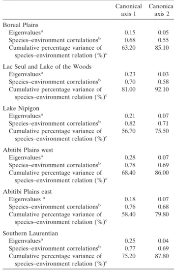
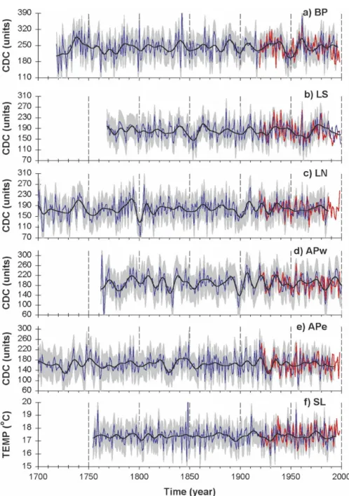
The regional drought reconstructions and their smoothed curves are shown in Fig. 4. Based on standard TABLE1. Redundancy analyses statistics per climate region.
Canonical axis 1 Canonical axis 2 Boreal Plains Eigenvaluesa 0.15 0.05 Species–environment correlationsb 0.68 0.55 Cumulative percentage variance of
species–environment relation (%)c
63.20 85.10
Lac Seul and Lake of the Woods
Eigenvaluesa 0.23 0.03
Species–environment correlationsb 0.70 0.58 Cumulative percentage variance of
species–environment relation (%)c
81.00 92.10
Lake Nipigon
Eigenvaluesa 0.21 0.07
Species–environment correlationsb 0.82 0.71 Cumulative percentage variance of
species–environment relation (%)c
56.70 75.50
Abitibi Plains west
Eigenvaluesa 0.28 0.07
Species–environment correlationsb 0.78 0.69 Cumulative percentage variance of
species–environment relation (%)c
68.40 86.00
Abitibi Plains east
Eigenvaluesa 0.18 0.07
Species–environment correlationsb 0.76 0.68 Cumulative percentage variance of
species–environment relation (%)c
58.40 79.80
Southern Laurentian
Eigenvaluesa 0.25 0.04
Species–environment correlationsb 0.77 0.69 Cumulative percentage variance of
species–environment relation (%)c
75.20 87.80
aVariance in a set of variables explained by a canonical axis. b Amount of the variation in species composition that may be
“explained” by the environmental variables.
cAmount of variance explained by the canonical axes as a fraction of the total explainable variance.
deviations of smoothed reconstructions ⬎1.0 for at least four consecutive years, persisting dry events marked the BP region during 1735–43, 1838–43, 1887– 92, 1936–40, and 1958–63. In the LS region, dry events marked 1791–95, 1838–42, 1860–67, 1908–11, 1932–37, and 1973–1983. In the APw and LN regions, dry events marked 1696–1700 (in LN), 1736–1744 (in LN), 1787– 96, 1806–10, 1836–41 (in APw), 1888–92 (in APw), 1905–11, 1918–22, 1934–38, and 1991–95. In the APe region, dry events marked 1734–38, 1748–54, 1789–92, 1819–22, 1837–49, and 1917–22. Warm spells occurred in the SL region during 1791–96, 1876–82, 1909–16, and 1971–78. Finally, the 1718–1840 period was marked by a significant positive correlation between the western (BP) and eastern (APe) regions [r ⫽ 0.24; 95% boot-strap confidence interval (0.09; 0.39)], contrasting with the absence of correlation from 1841 to 1984 (r⫽ ⫺0.12). A nonrotated PCA of the six drought reconstructions was run on the period 1768–1984; the first and second
component scores (PC1 and PC2, respectively) were projected on a time axis (Fig. 5). The relationship was extended to 1718 by running a second PCA on the BP, LN, and APe reconstructions on their common interval from 1718 to 1984. The component scores from this last PCA were highly correlated with the former ones (r
pc1⫽ 0.87 and rpc2⫽ 0.77 for n ⫽ 217, where n is the
sample size). The intent of this work was to focus on the west–east gradient, and thus succeeding PCs were not accounted for.
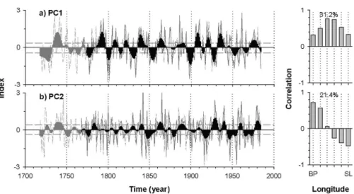
PC1 shared common variability with all six recon-structions; its center was located over Lake Nipigon and the western Abitibi Plains (Fig. 5a). The compo-nent showed strong interdecadal drought variability in the 1770–1845 and 1905–1940 intervals. Wavelet analy-sis (Fig. 6a) effectively indicated the presence of high variance in the 17–32-yr band (accounts for 20.3% of the variance). The spectrum also showed high variance in the 9–16-yr band in the early 1800s and early 1900s (Fig. 6a). Starting in the 1940s, variance in this band weakened, suggesting a change in the pattern of drought variability during recent decades.
The PCA orthogonality constraint in space generally dictates the second PC to be a domain-wide dipole (e.g., about half the dataset being inversely correlated with the component loading). PC2 was effectively associated with a dipole between the western and eastern regions and thus was referred to as a meridional component (Fig. 5b). Positive PC2 scores indicated drier conditions in the BP–LS regions and lower drought severity in the APe–SL regions, and vice versa. PC2 (Fig. 5b) sug-gested that the twentieth century was marked by an increase in the magnitude of the meridional compo-nent, particularly of its decadal mode. Interdecadal variability has also occurred during the periods of 1718– 50 and ⬃1830–70. Wavelet analysis (Fig. 6b) further indicated a period of increased variance in the 9–16-yr band during the late-twentieth century. Variance was also greater in the 17–32-yr band. The dynamics be-tween PC1 and PC2 and the atmosphere are analyzed in the subsection that follows.
d. Tropospheric circulation
Prior to investigating the composites, tests were con-ducted to validate the use of the 500-hPa geopotential heights against PC1 and PC2. (Refer to appendix C for a description of the climatology.) Correlation maps with 500-hPa geopotential heights (not shown) indi-cated that variability in PC1 was associated with a north and south dipole, with one cell at 57°N, 95°W and an-other at 35°N, 90°W. In contrast, the second PC was associated with an east and west dipole, with one cell at 50°N, 115°W and the other at 50°N, 50°W. The zonal FIG. 3. Transfer function model R2for the calibration period
1919–84 (black bars) and the corresponding RE statistics (gray bars) for the verification period of 1919–40, plotted against the time period for which a given calibration model was used (1941– 84). The R2is the fraction of the variance in instrumental data explained by the regression; the RE provides a sensitive measure of reconstruction reliability. Whenever RE is greater than zero the reconstruction is considered as being a better estimation of climate than the calibration period mean. The gray lines show the temporal developments of the number of chronologies used for the regional climate reconstructions (multiply the y scale by 50). Transitions from one submodel to another are delineated with vertical lines.
TABLE2. Relationships among reconstruction submodels per climatic regions. The values are Pearson correlation coefficients
cal-culated between submodels using the interval of 1870–1984. The labels in italic indicate the number of chronologies used in the submodels. Refer to Fig. 3 for identification of intervals covered by the submodels.
Pearson correlation coefficents
BP 5 6 8 10 11 13 5 1.00 6 0.95 1.00 8 0.91 0.95 1.00 10 0.87 0.91 0.88 1.00 11 0.86 0.89 0.87 0.98 1.00 13 0.84 0.84 0.82 0.87 0.88 1.00 LN 5 6 7 8 10 13 15 17 19 21 24 5 1.00 6 0.96 1.00 7 0.88 0.92 1.00 8 0.84 0.83 0.96 1.00 10 0.85 0.91 0.87 0.84 1.00 13 0.83 0.83 0.75 0.74 0.87 1.00 15 0.82 0.79 0.79 0.82 0.80 0.93 1.00 17 0.82 0.81 0.85 0.89 0.84 0.87 0.96 1.00 19 0.84 0.80 0.76 0.78 0.83 0.80 0.78 0.80 1.00 21 0.79 0.77 0.72 0.73 0.81 0.80 0.77 0.78 0.99 1.00 24* 0.78 0.75 0.69 0.70 0.80 0.79 0.75 0.77 0.98 0.99 1.00 APe 5 7 9 10 11 13 15 17 19 20 5 1.00 7 0.62 1.00 9 0.66 0.84 1.00 10 0.74 0.68 0.76 1.00 11 0.75 0.55 0.64 0.95 1.00 13 0.50 0.46 0.56 0.82 0.87 1.00 15 0.51 0.48 0.57 0.83 0.87 1.00 1.00 17 0.50 0.56 0.65 0.88 0.85 0.96 0.97 1.00 19 0.49 0.56 0.66 0.87 0.85 0.95 0.96 1.00 1.00 20* 0.39 0.61 0.64 0.78 0.72 0.75 0.76 0.83 0.85 1.00 LS 5 7 9 11 13 15 17 19 21 23 25 5 1.00 7 0.98 1.00 9 0.78 0.82 1.00 11 0.85 0.90 0.91 1.00 13 0.57 0.64 0.66 0.67 1.00 15 0.52 0.59 0.66 0.69 0.83 1.00 17 0.53 0.59 0.57 0.64 0.83 0.97 1.00 19 0.60 0.66 0.63 0.69 0.74 0.92 0.96 1.00 21 0.56 0.61 0.60 0.66 0.71 0.89 0.94 0.98 1.00 23 0.54 0.59 0.59 0.65 0.68 0.87 0.91 0.97 0.99 1.00 25 0.55 0.60 0.58 0.68 0.67 0.86 0.90 0.94 0.96 0.97 1.00 APw 6 7 9 10 11 12 13 6 1.00 7 0.69 1.00 9 0.66 0.73 1.00 10 0.64 0.72 0.98 1.00 11 0.64 0.71 0.97 1.00 1.00 12 0.65 0.72 0.98 1.00 1.00 1.00 13 0.64 0.71 0.98 0.99 0.99 1.00 1.00
index (ZI) and the meridional index (MI) define these types of circulation (after Bonsal et al. 1999):
ZI⫽ Grad共55⬚ to 65⬚N兲⫺ Grad共35⬚ to 45⬚N兲 共1兲 and
MI⫽ Z共45⬚ to 55⬚N, 115⬚W兲⫺ Z共45⬚ to 55⬚N, 80⬚W兲, 共2兲 where Z is the average 500-hPa value and Grad is the average 500-hPa gradient from 100° to 70°W (the ap-proximate longitudinal extent of the study region). The ZI measures the characteristic of the west–east flow over the six regions, where ⫹ZI defines a state with weak westerlies and strong meridional flow and⫺ZI is associated with strong westerlies and a weak meridional flow. The MI measures the meridionality of the flow, where⫹MI indicates an amplified western ridge and a deepened eastern trough and⫺MI indicates the reverse relation.
Time series of ZI and MI were correlated with their respective PC over the period of 1948–84 using the per-muted Pearson coefficients. Results indicated that PC1 depicted significant responses to the ZI (r⫽ 0.46, p ⬍ 0.005). Thus, it reflected variations in the strength of the westerly flow between the northern (55°–65°N) and southern (35°–45°N) regions. PC2 correlated well with the MI (r⫽ 0.45, p ⬍ 0.005), indicating that it reflected variations in the western ridge and eastern trough. These results were comparable to calculations on PCs obtained from instrumental records over the interval of 1948–98 (ZIpc1⫽ 0.41, MIpc2⫽ 0.43).
Years of highest and lowest PC1 and PC2 scores were selected for the creation of 500-hPa geopotential height and vector wind anomaly composites (1948–84 period). A two-sample permutation test indicated a significant difference in means among samples of ZI indices at the
time of the five highest and five lowest PC1 scores ( p⫽ 0.016). Similarly, a significant difference in means was observed among MI samples of the highest and lowest PC2 scores ( p⫽ 0.009). These two tests validated the use of the composite maps for exploration of the midtropospheric circulation variability associated with PC1 and PC2.
The 5 yr of positive PC1 (dry years; Fig. 7a) were associated, on average, with intensified ridging over the western Hudson Bay, lower-level divergence, and sub-sidence over much of the boreal forest (giving rise to drier conditions particularly in LN, APw, and APe re-gions). A meridional component gave rise to northeast-erly winds in eastern Canada and southnortheast-erly winds in the Great Plains. The 5 yr of⫺PC1 (Fig. 7b) were associ-ated with lower heights over boreal Canada. As op-posed to positive PC1 scores,⫺PC1 scores were asso-ciated with stronger midtropospheric westerlies and an amplified jet stream at 45°N and 70°–110°W. During years of low drought severity, moisture-bearing systems from the North Pacific Ocean were free to move across the continent. At 60°N the situation was the opposite, with the near absence of mid- and high zonal tropo-spheric winds (in absolute chart-reduced westerlies, not shown).
PC2 was, on average, associated with an oscillation in the position and direction of the jet stream and meridi-onal flows from westward (positive PC2) to eastward (⫺PC2). Positive PC2 scores (Fig. 7c) were character-ized by ridging over the Gulf of Alaska and Greenland and intensified troughing in eastern Canada. An anomalous anticyclonic flow over the Rocky Moun-tains, combined with the cyclonic flow above Ontario, gave rise to midtropospheric northwesterlies over cen-tral Canada and western Ontario. The persistence of the ridge induced subsidence of air over the eastern Boreal Plains, low precipitation, warming, and drying. TABLE2. (Continued)
Pearson correlation coefficents
SL 5 7 9 11 13 19 21 23 25 5 1.00 7 0.93 1.00 9 0.80 0.80 1.00 11 0.85 0.79 0.87 1.00 13 0.84 0.79 0.83 0.94 1.00 19 0.85 0.89 0.79 0.87 0.89 1.00 21 0.82 0.80 0.78 0.93 0.88 0.90 1.00 23 0.81 0.83 0.77 0.85 0.82 0.90 0.94 1.00 25 0.83 0.87 0.81 0.85 0.85 0.91 0.89 0.89 1.00
* These LN (1869–1987) and APe (1832–1984) submodels (RE⫽ 0.17 and 0.26, respectively) were not included in the final recon-structions; their statistics were omitted from Fig. 3.
In eastern Canada, the cyclonic activity drove midtro-pospheric southerlies along the U.S. east coast toward the Quebec interior. This flow allowed the advection of warm, moist, and unstable air from the subtropical North Atlantic basin into Quebec. The 5 yr of ⫺PC2 (Fig. 7d) were associated with a weakening of the
east-ern trough, and a downstream convergence and subsi-dence zone near 70°W. The circulation was associated with southerlies in the Boreal Plains and western Bo-real Shield that brought moisture-rich air from the coastal subtropical North Pacific. In eastern Quebec the anticyclonic flow drove an outflow of dry arctic air. FIG. 4. Reconstructions of the mean July CDC (units) for the (a) BP, (b) LS, (c) LN, (d)
APe, and (e) APw regions. The CDC scale ranges from soil saturation (zero) to extreme drought (⬎300). (f) Reconstruction of the SL mean July–August temperature (°C). Shaded area: error bars plotted against the time period for which a given calibration model was used. Red lines show instrumental 1913–98 records. Variance in the instrumental records was adjusted to correspond to reconstructions. Smoothed curves (black lines) were obtained from a polynomial fitting (order 6) across a moving 10-yr window within the data. These curves accounted for (a) 22.0%, (b) 22.8%, (c) 24.9%, (d) 35.1%, (e) 19.2%, and (f) 8.1% of the variance in the reconstructions.
FIG. 5. (a) PC1 and (b) PC2 scores of the PCA (thin solid lines) illustrating the relationship among the six climate reconstructions over the common interval of 1768–1984. The vertical bar charts at right express the correlation coefficients between a PC score and a given climate reconstruction (BP for western and SL for eastern sectors); the percentage of expressed variance by the PC scores is indicated. Also projected are the PC scores covering the interval of 1718–67 (thin dashed lines) obtained from the BP, LN, and APe reconstructions. Smoothed PC scores are overlaid in black.
FIG. 6. Continuous wavelet transformation power spectrums of (a) PC1 and (b) PC2. The dark blue color indicates areas of large power; thick-red contour is the 5% significance level for red noise [AR(1)⫽ 0.25 in (a) and AR(1) ⫽ 0.00 in (b)]. The cross-hatched regions on either end delineate the cone of influence where zero padding has reduced the variance. Note that for the period of 1718–67 the PCs were computed from only three climate reconstructions (BP, LN, and APe).
The PCs are additive, so any pattern from PC1 (ei-ther Fig. 7a or 7b) can be superimposed on any pattern from PC2 (Fig. 7c or 7d). For instance, PC1 indicated that 1955 was generally dry over the LS, LN, and APw regions. PC2 indicated that it was drier in APe than in BP. Climatologically, this suggested that the circulation in 1955 featured a strong anticyclone (i.e., Fig. 7a), but with a center located northeast of Ontario.
e. Sea surface temperatures
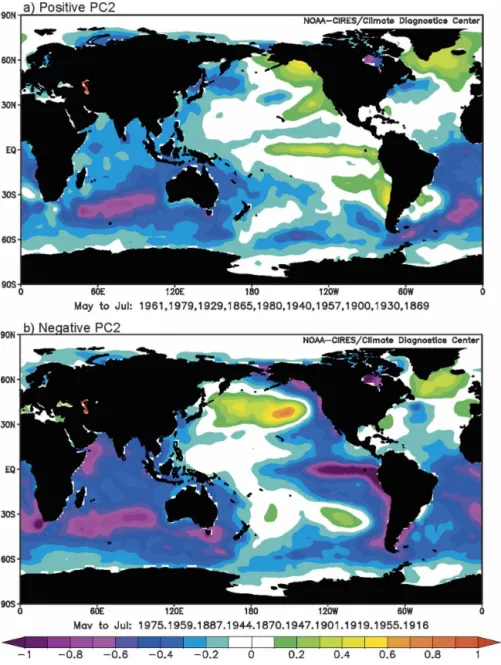
The connection between the west–east meridional component (PC2) and global ERSST is presented in Fig. 8. Analyses conducted on PC1 show no significant correlation with the mean May–July SST, and thus are not presented. A PC2 correlation chart (not shown) indicated a significant positive correlation ( p ⬍ 0.05) with SST along the eastern North Pacific coast and into the Tropics. A center of significant negative correlation was also observed in the interior North Pacific, roughly at 160°W and 30°N. The spatial structure of the vari-ability was very similar to that of the Southern Oscilla-tion (Ropelewski and Jones 1987), but with greater am-plitude at high latitudes and a reduced tropical expres-sion. The Pacific pattern is the one commonly referred
to as the Pacific decadal oscillation (PDO; Mantua et al. 1997; Zhang et al. 1997) or North Pacific pattern (Latif and Barnett 1996). A significant Pearson correlation between PC2 and the May–July ERSST PDO of Smith and Reynolds (2003; not shown) was obtained [r⫽ 0.25 with 95% confidence interval (0.09; 0.39), period 1854– 1984]. Analysis between the PDO and PC2 10–30-yr/ cycle waveforms (not shown) further indicated a highly significant correlation in the interdecadal mode with
r⫽ 0.72 (0.64; 0.79). [Correlations were computed
us-ing a nonparametric stationary bootstrap that accounts for autocorrelation in the data (PearsonT software; Mudelsee 2003).]
A two-sample permutation test indicated a signifi-cant difference in means among samples of ERSST PDO indices at the time of the 10 highest and the 10 lowest PC2 scores ( p⬍ 0.004). Figure 8a indicated that positive PC2 were associated with higher SSTs along the western coast of North America. A center of posi-tive anomalies not dissimilar to the typical El Niño sig-nature, but with reduced expression, was also observed in the tropical Pacific, roughly at 150°W. Two centers of lower-than-normal SSTs were observed in the interior North Pacific near 37°N, 160°W, and in the western FIG. 7. May–July 500-hPa geopotential height anomaly composites (5-m contour intervals) for 5 yr of (a) highest PC1 scores, (b) lowest PC1 scores, (c) highest PC2 scores, and (d) lowest PC2 scores. Regions of anomalously low (LOW) and high (DRY) drought severities are indicated. Solid contours indicate positive anomalies; dashed contours indicate negative anomalies (zero interval is boldface). Directions of 500-hPa vector wind anomalies (arrows) are also shown. The anomalies were calculated from the mean of the reference period of 1968–96. Years used in the composites are listed below each map.
North Pacific near 45°N, 155°W (Fig. 8a). In the South Pacific, a similar pattern was observed, with warmer SSTs along the American coast.
During average PC2 scores (not shown), the interior North Pacific anomaly shifted in sign. Lower SST oc-curred in the tropical and east subtropical North Pacific and along the western coast of North America and South America. During negative PC2 scores (Fig. 8b), the center of anomalously positive SSTs in the interior North Pacific intensified. SSTs lowered to reach an av-erage of ⬃1.5°C below normal in the eastern tropical and subtropical North Pacific (the typical La Niña
sig-nature) and ⬃0.7°C below normal along the western coast of Alaska. In the South Pacific, a similar pattern was observed, with warmer SSTs in the interior and cooler SSTs along the South American coast.
f. Frequency of composite types
Histograms showing the frequency per decades of positive and negative PC score departures were created (Fig. 9). The PC scores were classified as being either part of the upper 33.3% percentiles (positive PC tures), lower 33.3% percentiles (negative PC depar-tures), or in between (residual PC departures). The FIG. 8. May–July SST anomaly composites for 10 seasons of (a) highest PC2 scores and (b)
lowest PC2 scores over the interval of 1854–1984. The anomalies were calculated from the mean of the reference period of 1971–2000. Years used in the composites are listed below each map.
33.3% percentile threshold was arbitrarily chosen and results were consistent with the 20.0% and 40.0% thresholds.
The temporal distribution of the PC2 scores sug-gested a period of less frequent positive PC2 from 1751 to 1850, with the exception of the intervals of 1781–1800 and 1821–40. The 1751–1850 interval contrasted with periods of frequent positive PC2 from 1721–50 and 1851–1940 (Fig. 9d). From 1751 to 1850, positive PC2 occurred at an average rate of 2.3 yr decade⫺1, whereas from 1851 to 1940 the average was 4.1 yr decade⫺1. This change in the frequency of occurrences of positive PC2 in 1850 was tested significant using a two-sample per-mutation test ( p⫽ 0.006). A significant change toward a reduced frequency in the residuals of PC2 (Fig. 9f) from the former period to the later was also detected ( p⫽ 0.018). No significant change was detected in the frequency of PC1 and negative PC2 departures.
Climatologically, this change in the frequency of PC2 scores suggested a period of greater zonality from 1751 to 1850 across the eastern Boreal Plains and Boreal Shield during the summertime. It implied that less fre-quent ridging and air subsidence marked 1751–1850 over the eastern Boreal Plains, while in the eastern Boreal Shield it meant a weaker trough and less fre-quent advection of humid air masses from the subtropi-cal North Atlantic. The midtropospheric pattern asso-ciated with Fig. 7c and the SST pattern assoasso-ciated with Fig. 8a (cooler SST in the interior North Pacific and
warmer ones along the American North Pacific coast and in the Tropics) were likely less frequent from 1751 to 1850. The atmospheric transition at⬃1850 is further investigated in the next subsection.
g. Validation of spatiotemporal variability
The temporal stability of the shared variance among regions was evaluated by conducting a PCA on a rect-angular matrix of 90 multicentury tree-ring residual chronologies, sharing the common period of 1781–1980, and distributed across a rectangular grid covering from 41° to 61°N and from 101° to 61°W (Fig. 10) (e.g., Fritts et al. 1991; Bradley 1999; Gajewski and Atkinson 2003; Tardif et al. 2003). The rectangular matrix was created by nesting 58 chronologies located within our six cli-mate regions into a grid composed of 32 chronologies from surrounding areas (Fig. 1; appendix A). All mea-surement series were processed as described in section 2b. The 1781–1980 period was chosen to maximize the length of the period of analysis, the number of chro-nologies in each region, and the subsignal strength. The shared variance was analyzed by constructing four se-quential maps, each one representing the chronology loadings on a principal component for a given period of 100 yr. Though species were unequally distributed in the area of study, the approach was justified by the persistence of the relationship between radial growth and climate in the six regions.
The analysis of the interval of 1781–1880 (Fig. 10a) FIG. 9. Histograms showing the frequency per decade of PC1 and PC2 positive and negative
departures exceeding the higher and lower 33.3% percentiles from the long-term mean of the reference period of 1718–1984. The frequency per decade of nondeparture years (PC residu-als) is also shown. Third-order polynomial regression lines accounting for (d) 22.6% and (f) 20.4% are shown. PCs were obtained from the analysis of the BP, LN, and APe reconstruc-tions.
indicated that in the earliest period, chronologies from all sectors shared common variance. After 1851, a breakup of the common signal was observed with the weakening of the correlation coefficients between PC1 and chronologies from northern Canada and Quebec. This transition from a domain-wide pattern to a dipole likely reflects a shift in midtropospheric wind flow be-tween the north and south. The percentage of ex-plained variance has not changed substantially from the first interval to the last.
In the earliest interval, PC2 (Fig. 10b) was character-ized by a north–south dipole with the axis (zero line) passing through approximately 55°N. The dipole was weak on its negative center (average correlation ⬎⫺0.20) and strong on its positive one (average corre-lation⬍0.45). In the interval after 1851, the orientation
of the dipole shifted toward a west–east direction with the axis passing through approximately 90°W, that is, just west of Lac Seul. This is the current location of the average summer position of the axis dividing the west-ern ridge from the eastwest-ern trough (refer to Figs. 7c–d).
4. Discussion
a. Atmospheric circulation
The presented analyses provide new information on the year-to-year and decade-to-decade variability of summer drought severity along the southern limit of the Canadian boreal forest. Results suggest that the area covering the eastern Boreal Plains to the eastern Boreal Shield is under the influence of two components of large-scale atmospheric circulation. The zonal compo-FIG. 10. Spatial correlation fields of (a) PC1 and (b) PC2 of the 90 tree-ring chronologies for different 100-yr time periods. The respective eigenvalues are shown (%). Centers of positive (H) and negative (L) correlation are indicated. The total sum of the squares of the data matrix for each time period is 262.1, 236.2, 209.6, and 218.6, respectively. PCA was conducted using the correlation matrix.
nent (PC1) is associated with a circulation of cool and moist westerlies over the central area of the Boreal Shield during years of low drought severity, and a cir-culation of dry and cold northerlies during years of high drought severity. The analysis of the component’s spec-tra showed high variance in the 17–32-yr band over most of the reconstructed period. The analysis revealed no major changes in either its magnitude at⬃1850, or in its spectra. Changes were, however, noted in other pe-riods, with strong variance in high-frequency bands around 1800 and 1900 and low variance in the late-twentieth century. Despite the absence of changes in the component in⬃1850, analysis of the spatiotemporal variability in radial growth over the eastern half of Canada and the United States suggested that the ex-pression of the zonal pattern has changed between the northern and the southern areas of the Boreal Shield. This shift would corroborate with the reported contrac-tion of the Aleutian and Icelandic lows in 1850 (Guiot 1985; Gajewski and Atkinson 2003).
The meridional component reflects regional drought variability in the west–east dimension. This variability occurs as a response to the blocking of moisture-carrying systems upstream and advection of moisture air downstream of the long waves (Flannigan and Har-rington 1988; Weber 1990; Knox and Lawford 1990; Bonsal et al. 1999; Skinner et al. 1999, 2002). An am-plified western ridge is associated with a northerly dis-placement of the jet stream over western Canada and a southerly displacement in eastern Canada. This con-figuration favors northerly winds, air subsidence, and increasing drought severity in the eastern Boreal Plains. In the eastern Boreal Shield, this configuration favors cyclonic development, inflows of subtropical North At-lantic air, and lower drought severity. Spatiotemporal analyses conducted on the six reconstructions and the multicentury tree-ring chronologies suggested that the meridional component has gained in magnitude over the past 150 yr and particularly in the decadal scale of variability. This suggested that more intense longwave oscillations occurred during the past century over the Canadian boreal forest, contributing to a greater con-trast in summer drought severity between the eastern Boreal Plains and eastern Boreal Shield. Analyses of year-to-year variability suggested that from ⬃1751– 1850, amplifications of the western ridge and eastern trough were likely infrequent relative to ⬃1851–1940 (Fig. 9c). This meant reduced frequency in the occur-rence of air subsidence in the eastern Boreal Plains and airmass advection in the eastern Boreal Shield during the former interval.
Skinner et al. (1999) addressed the effect of atmo-spheric circulation shifts on the area burned across
Canada. A transition toward a higher frequency of ridg-ing (troughridg-ing) over western (eastern) Canada after 1974 contributed to significant increases in the area burned, especially in the northwest and central regions (1975–95 versus 1953–74). Analyses by Girardin et al. (2004b) effectively showed significant correlations be-tween seasonal area burned across the six regions dur-ing the period of 1959–98 and the instrumental zonal PC1 and meridional PC2. However, despite the fact that the season covered by the reconstructions may be a good proxy for fire weather conditions at the time of the greatest area burned, it may underestimate or omit variability and temporal changes in conditions leading to spring and late-summer fires. In Canada, 78% of the area burned from 1959 to 1998 occurred in June and July, while 8% occurred during May and 13% during August (Stocks et al. 2003).
The temporal changes reported are in the year-to-year and decade-to-decade scales of variability. Little attention was given to the reconstruction of low-frequency variations. In the past year or so discussions have taken place regarding various methods applied to standardize tree-ring data (e.g., Esper et al. 2002). The debate is focused on differencing the long-term climate signal from the long-term tree growth signal. For in-stance, the different approaches of tree-ring data stan-dardization appear to most substantially account for the differing low-frequency trends in the reconstructed Northern Hemisphere temperature (Esper et al. 2002). The use of nonconservative detrending may however be increasingly important in tree-ring data showing noise resulting from stand disturbances (herbivory and post–forest fire growth releases). But most importantly, the period covered by most samples collected in the boreal forest is insufficiently long to allow for robust reconstruction of low-frequency variations. The contri-bution of other types of proxies could be valuable in attempting to reconstruct low-frequency changes that may superimpose on those reported in this work.
b. North Pacific air–sea interactions
It is now commonly accepted that the atmospheric response to SST anomalies in the equatorial Pacific de-termines ocean conditions over the remainder of the global ocean (Yang and Zhang 2003; Kumar and Ho-erling 2003; Lau et al. 2004; Shabbar and Skinner 2004). Tropical SSTs, with the contribution of stochastic feed-back from the atmosphere, generate the North Pacific SST anomalies (Schneider et al. 2002; Newman et al. 2003; Wu and Liu 2003). Wu and Liu (2003) indicated that anomalies in the central and eastern North Pacific Ocean, well simulated by global ocean–atmosphere models, could be obtained from anomalous Ekman
transport and surface heat flux. Lau et al. (2004) sug-gested a mechanism in which air–sea interactions am-plify North Pacific anomalies and sustain them through feedback processes, involving the interplay of surface fluxes, atmospheric mean circulation and transient ed-dies, and radiation effects of stratocumulus cloud decks. Several paleoclimate studies suggested important changes in the North Pacific climate over the past three centuries (Luckman et al. 1997; Stahle et al. 1998; D’Arrigo et al. 2001; Evans et al. 2002; Finney et al. 2000; Gedalof et al. 2002; Wilson and Luckman 2003). The significant association observed between the me-ridional component and tropical and North Pacific SSTs indicated that spatiotemporal drought variability over the eastern half of Canada has been under the influence of this coupling for a period covering at least 150 yr. Because of the relationship between Pacific SSTs and atmospheric circulation, the combined infor-mation from these studies could support the observa-tion of a weakened western ridge and eastern trough from⬃1760 to 1840. Investigation of prominent aquatic population declines in the Gulf of Alaska by Finney et al. (2000) suggested the prevalence of cooler water along the coast from approximately 1750 to 1850. A prolonged period of cooler Pacific and western coast air temperature during the preindustrial period was also reported by Luckman et al. (1997), D’Arrigo et al. (2001), Evans et al. (2002), and Wilson and Luckman (2003). Reconstruction of the Southern Oscillation in-dex (SOI) by Stahle et al. (1998) showed a statistically significant increase in the SOI interannual variability during the mid-ninetieth century. Though there may be a teleconnection, the meridional component developed here is not optimized to capture the maximum atmo-spheric circulation variability associated with the Pa-cific, and thus it should not be interpreted as a proxy for past SST variability.
This study may be complementary to recent work by Jacobeit et al. (2003) in which July dynamical modes of atmospheric circulation in Europe were reconstructed. The authors also observed a period dominated by a westerly flow from about 1750 toward the end of the nineteenth century. Thereafter, a steady increase of a meridional component followed, which was associated with increasing anticyclonic activity over the eastern North Atlantic and the European continent. While it is difficult to link European and Canadian climate vari-ability, the combined information from this study and that of Jacobeit et al. (2003) suggests that the circula-tion transicircula-tion at about 1850 from zonal to meridional flows could be part of a global-scale phenomenon. In the context of global ocean teleconnections, it is sug-gested that North Pacific and North Atlantic SST
pat-terns may be connected through an extratropical cli-mate mode, linking SST variability in the North Pacific and the North Atlantic via an atmospheric bridge across North America (Lau et al. 2004).
c. Concluding remarks
This work constitutes an important step in the devel-opment of climate change adaptation strategies in the Canadian boreal forest sector. Paleoclimate informa-tion can improve our understanding of how the atmo-sphere–ocean and land climate systems have evolved over the past centuries, and provide a baseline to an-ticipate future vegetation response to climate variabil-ity and change across Canada. The results suggest that broad-scale atmospheric circulations are important in meteorological conditions like drought. Fire is related to weather, and more specifically drought, so it is likely that uncovered atmospheric patterns have also influ-enced forest fires and vegetation dynamics over the past centuries. In the light of the present findings, it is pertinent to believe that the decrease in the frequency of large areas burned around 1850 on the eastern Ca-nadian Boreal Shield is because of the more frequent advection of air masses from the subtropical North At-lantic. The meridional circulation is however highly variable in the decadal scale, and this variability likely gave rise to several succeeding episodes of severe and prolonged midtropospheric circulation blocking during the past 80 yr or so.
Acknowledgments. We acknowledge the Sustainable
Forest Management Network for funding this research and supporting M. P. Girardin. The author was also supported by doctoral scholarships from the Fonds Québécois de la Recherche sur la Nature et les Tech-nologies and the Prairies Adaptation Research Col-laborative. The field and laboratory work for the de-velopment of the Ontario chronologies could not have been done without the incredible support of Elizabeth Penner and Daniel Card. We thank Ontario Provincial Park for granting us permission to conduct this research in their parks. Thanks to Stan Vasiliauskas, Ed Iskra, Don Armit, Charlotte Bourdignon, and Dave New from the Ontario Ministry of Natural Resources and Timothy Lynham from the Canadian Forest Service for making our search of old trees in Ontario successful. We thank NOAA (NCEP–NCAR reanalysis project) and the Meteorological Service of Canada for their aid and contribution of climate data. We thank Kim Mon-son, Danny Blair, Malcom Cleaveland, and two anony-mous reviewers for commenting on and editing the manuscript.
APPENDIX A
Sources of Tree-Ring Chronologies
TABLEA1. Sources of the tree-ring chronologies. Mean is mean length of measurement series; N is the sample depth of the tree-ring series; SSS is the subsample signal strength and is used to define the portion of the residual chronology (year y to present) with a strong common signal (Wigley et al. 1984); and Sens is mean sensitivity of the residual chronology, with NA for information not available.
Species Contrib-utors* Location Lat (°N) Lon (°W) Period Mean (yr) N SSS ⬎ 0.85 (yr) Sens Boreal Plains
1 Quercus macrocarpa Ss Red River Alluvial Logs 49.20 97.10 1448–1999 98 92 1523 0.19
2 Quercus macrocarpa Ss Kildonan Park 49.56 97.06 1720–1999 137 44 1851 0.24
3 Thuja occidentalis Tj Middlebro 49.27 95.23 1802–2003 130 20 1875 0.16
4 Thuja occidentalis Tj Cedar Lake 53.00 99.16 1713–1999 117 77 1811 0.14
5 Pinus resinosa Tj Black Island 51.10 96.30 1709–2001 102 148 1724 0.15
6 Larix laricina Tj Duck Mountain Provincial Forest 51.60 101.00 1676–2002 99 89 1729 0.21 7 Picea mariana wet Tj Duck Mountain Provincial Forest 51.60 101.00 1758–2001 177 64 1795 0.13 8 Picea mariana dry Tj Duck Mountain Provincial Forest 51.60 101.00 1724–2000 156 19 1895 0.16 9 Pinus banksiana Tj Duck Mountain Provincial Forest 51.60 101.00 1717–2001 87 521 1757 0.15 10 Picea glauca Tj Duck Mountain Provincial Forest 51.60 101.00 1776–2001 129 81 1829 0.18 11 Populus balsamea Tj Duck Mountain Provincial Forest 51.60 101.00 1808–2001 106 47 1890 0.28 12 Populus tremuloides Tj Duck Mountain Provincial Forest 51.60 101.00 1806–2001 94 264 1888 0.25 13 Betula papyrifera Tj Duck Mountain Provincial Forest 51.60 101.00 1785–2001 102 114 1893 0.24 Lac Seul Upland and Lake of the Woods
14 Picea glauca Sf Bruno Lake 51.37 95.50 1822–1988 126 24 1846 0.19
15 Picea glauca Sf High Stone Lake 50.24 91.27 1813–1988 130 25 1827 0.18
16 Pinus resinosa Gm Caliper Lake Provincial Park 49.05 93.92 1851–2001 134 17 1857 0.20
17 Pinus resinosa Gm Kenora 49.92 94.12 1792–2001 129 41 1828 0.16
18 Pinus resinosa Gm Sioux Lookout Provincial Park 49.42 94.05 1772–2001 134 44 1808 0.23
19 Pinus strobus Gm Longbow Lake 49.72 94.28 1789–2002 123 41 1844 0.21
20 Pinus resinosa Gm Longbow Lake 49.72 94.28 1830–2001 157 43 1836 0.23
21 Pinus banksiana Gm Highway 105 50.45 93.12 1815–2001 130 44 1818 0.19
22 Pinus banksiana Gm Lake Packwash Provincial Park 50.77 93.43 1852–2001 86 12 1872 0.21 23 Pinus resinosa Gm Lake Packwash Provincial Park 50.75 93.43 1744–2002 168 38 1823 0.20
24 Pinus strobus Gm Camping Lake 50.58 93.37 1827–2002 112 37 1857 0.17
25 Thuja occidentalis Gm Lac Seul south 50.27 92.28 1762–2002 110 42 1875 0.17
26 Pinus resinosa Gm Lac Seul south 50.32 92.28 1837–2001 132 40 1855 0.12
27 Pinus resinosa Gm Red Lake 51.08 93.82 1818–2001 155 41 1823 0.18
28 Pinus banksiana Gm Snail Lake 50.87 93.38 1847–2002 91 24 1898 0.17
29 Pinus resinosa Gm Stormy Lake 49.35 92.23 1791–2001 112 37 1812 0.14
30 Pinus strobus Gm Eagle Lake 49.77 93.33 1712–2002 126 40 1765 0.22
31 Pinus resinosa Gm Eagle Lake 49.78 93.33 1808–2001 146 39 1825 0.18
32 Pinus strobus Gm Sioux Lookout 50.07 91.92 1784–2002 112 40 1848 0.17
33 Pinus resinosa Gm Sioux Lookout 50.07 91.92 1766–2002 116 29 1807 0.18
34 Pînus resinosa Gm Sowden Lake 49.53 91.17 1640–2001 216 40 1738 0.15
35 Pînus strobus Gm Sowden Lake 49.53 91.17 1816–2002 110 39 1836 0.18
36 Pinus strobus Gm Turtle River Provincial Park 49.25 92.22 1810–2001 104 34 1834 0.15 37 Pinus resinosa Gm Lake Sandbar Provincial Park 49.45 91.55 1828–2000 100 35 1899 0.19 38 Pinus strobus Gm Lake Sandbar Provincial Park 49.45 91.55 1773–2002 104 54 1902 0.18 Lake Nipigon
39 Pinus resinosa Gl Saganaga Lake 48.00 90.00 1719–1988 188 43 1780 0.23
40 Pinus resinosa Sc Ed Shave Lake 48.00 91.00 1700–1982** 162 38 1797 0.24
41 Pinus resinosa Gl Saganaga Lake 48.13 90.54 1644–1988 201 51 1693 0.26
42 Betula papyrifera Gm Rainbow Fall Provincial Park 48.50 87.38 1766–2001 143 48 1783 0.33 43 Picea glauca Gm Rainbow Fall Provincial Park 48.50 87.38 1788–2001 122 58 1813 0.19 44 Thuja occidentalis Gm Rainbow Fall Provincial Park 48.50 87.38 1774–2001 141 42 1825 0.15
45 Pinus strobus Gm Nipigon 49.23 88.17 1833–2002 98 47 1861 0.17
46 Pinus banksiana Gm Lake Nipigon Provincial Park 49.45 88.12 1866–2001 101 30 1875 0.16
47 Pinus banksiana Gm Shakespeare Island 49.62 88.08 1864–2002 83 62 1871 0.14
48 Thuja occidentalis Gm Beardmore campground 49.53 87.82 1734–2001 141 56 1819 0.15
TABLEA1. (Continued) Species Contrib-utors* Location Lat (°N) Lon (°W) Period Mean (yr) N SSS ⬎ 0.85 (yr) Sens 50 Picea glauca Gm MacLeod Provincial Park 49.68 87.90 1804–2000 140 50 1835 0.15 51 Thuja occidentalis Gm MacLeod Provincial Park 49.68 87.90 1790–2001 116 43 1859 0.14 52 Thuja occidentalis Gm Upper Twin Lake 50.15 86.55 1772–2001 124 32 1842 0.17 53 Picea mariana Gm Upper Twin Lake 50.15 86.55 1797–2002 150 39 1812 0.13 54 Pinus banksiana Gm Longlac 49.67 86.22 1847–2001 105 34 1864 0.21 55 Picea mariana Gm Sleeping Giant Provincial Park 48.37 88.82 1676–2001 132 30 1785 0.16 56 Pinus banksiana Gm Sleeping Giant Provincial Park 48.47 88.73 1817–2001 101 35 1826 0.18 57 Thuja occidentalis Gm Sleeping Giant Provincial Park 48.45 88.73 1713–2001 140 33 1828 0.13 58 Pinus resinosa Gm Sleeping Giant Provincial Park 48.45 88.73 1805–2001 159 41 1817 0.19 59 Pinus strobus Gm Sleeping Giant Provincial Park 48.45 88.73 1805–2001 116 42 1840 0.16 60 Pinus strobus Gm Sleeping Giant Provincial Park 48.43 88.75 1807–2001 145 53 1814 0.17 61 Thuja occidentalis Gm Sleeping Giant Provincial Park 48.37 88.82 1662–2001 162 55 1746 0.12 62 Thuja occidentalis Gm Sleeping Giant Provincial Park 48.32 88.87 1665–2001 137 68 1824 0.14 Abitibi Plains west
63 Thuja occidentalis Gm Fushimi Lake Provincial Park 49.83 83.92 1765–2002 154 34 1815 0.14 64 Picea mariana Gm René-Brunelle Provincial Park 49.42 82.13 1721–2002 148 50 1790 0.13 65 Pinus strobus Gm Geiki Lake 48.18 81.08 1709–2002 96 41 1876 0.17 66 Pinus resinosa Gm Blue Lake 48.58 81.72 1606–2002 223 46 1772 0.19 67 Pinus banksiana Gm Blue Lake 48.58 81.72 1760–2002 156 55 1772 0.17 68 Pinus banksiana Gm Foliyet 48.23 82.00 1769–2002 113 30 1819 0.17 69 Pinus resinosa Gm Ivanhoe Lake Provincial Park 48.15 82.50 1828–2002 126 38 1848 0.17 70 Thuja occidentalis Gm Missinaibi Provincial Park 48.27 83.40 1798–2002 128 43 1842 0.17 71 Pinus resinosa Gm Highway 556 46.87 83.45 1837–2002 144 33 1848 0.14 72 Thuja occidentalis Gm Highway 556 46.88 83.43 1760–2002 130 44 1827 0.17 73 Pinus strobus Gm Ranger Lake 47.02 83.88 1760–2002 99 40 1823 0.22 74 Pinus strobus Gm Montreal River 47.22 84.63 1779–2002 117 33 1880 0.20 75 Pinus resinosa Gm Montreal River 47.22 84.65 1773–2003 158 37 1780 0.28 Abitibi Plains east
76 Pinus strobus Gr Hobbs Lake 46.43 80.12 1547–1994 212 31 1714 0.16 77 Pinus resinosa Ce Lac Temagami 47.00 79.00 1644–1983** 266 36 1690 0.18 78 Populus tremuloides Cd Lac Duparquet 48.28 79.19 1831–1996 146 30 1840 0.24 79 Betula papyrifera Cd Lac Duparquet 48.28 79.19 1766–1998 138 74 1804 0.25 80 Picea mariana Gm Lac Duparquet 48.28 79.19 1800–1999 126 61 1849 0.14 81 Fraxinus nigra Tj Lac Duparquet 48.28 79.19 1790–1991 100 36 1834 0.20 82 Fraxinus nigra Tj Lac Duparquet 48.28 79.19 1682–1991 134 253 1716 0.20 83 Thuja occidentalis As Lac Duparquet 48.28 79.19 1186–1987 507 46 1283 0.16 84 Thuja occidentalis Tj Lac Duparquet 48.28 79.19 1417–1987 302 43 1569 0.14
85 Picea mariana Ha Joutel 49.26 78.27 1778–1994 NA 57 NA 0.18
86 Picea mariana Ha Hedge Hills 49.16 78.24 1816–1992 NA 67 NA 0.17 87 Picea mariana Ha Chicobi Hills 48.51 78.38 1820–1994 NA 61 NA 0.16 88 Picea mariana Ha Lac Opasatica 48.06 79.18 1703–1994 NA 61 NA 0.17 89 Picea mariana Ha Lac Hébécourt 48.29 79.27 1790–1993 NA 59 NA 0.17 90 Pinus banksiana By Abitibi Lake 49.00 79.50 1713–1987 103 75 1732 0.17 91 Pinus banksiana By Lac Duparquet 48.28 79.19 1726–1985 97 94 1775 0.16
92 Pinus banksiana Ha Joutel 49.26 78.27 1714–1994 NA 51 NA 0.19
93 Pinus banksiana Ha Hedge Hills 49.16 78.24 1811–1992 NA 67 NA 0.22 94 Pinus banksiana Ha Chicobi Hills 48.51 78.38 1814–1994 NA 57 NA 0.19 95 Pinus banksiana Ha Lac Hébécourt 48.29 79.27 1776–1993 NA 49 NA 0.22 Southern Laurentian
96 Picea mariana GsDl Lac Dionne 49.52 67.76 1809–1999 166 40 1824 0.13 97 Picea mariana GsDl Lac Dionne 49.66 67.58 1743–1999 181 48 1803 0.16 98 Pinus banksiana GsDl Lac Dionne 49.52 67.76 1811–1998 133 21 1817 0.16 99 Abies balsamea KcMh Mont Valin 48.05 70.04 1789–1994 NA NA NA NA 100 Picea mariana KcMh Cote-Nord 30 49.05 69.03 1713–1996 NA NA NA NA 101 Pinus strobus KcGf St-Marguerite 48.02 70.00 1768–1995 133 12 1850 0.17 102 Picea mariana Sf Lac Chevrillon 50.01 74.27 1797–1988 87 37 1813 0.14 103 Abies balsamea KcMh Lac Liberal 49.04 72.06 1751–1995 NA NA NA NA