is an open access repository that collects the work of Arts et Métiers Institute of
Technology researchers and makes it freely available over the web where possible.
This is an author-deposited version published in: https://sam.ensam.eu
Handle ID: .http://hdl.handle.net/10985/11474
To cite this version :
François MALBURET, Jean-Claude CARMONA, Benjamin BOUDON - Simulation of a
helicopter’s main gearbox semiactive suspension with bond graphs - Multibody System Dynamics - Vol. 39, n°1, p.60-64 - 2016
Any correspondence concerning this service should be sent to the repository Administrator : archiveouverte@ensam.eu
Simulation of a helicopter’s main gearbox semi-active suspension
with bond graphs
Benjamin BOUDON, François MALBURET, Jean-Claude CARMONA
Abstract
This paper presents a bond graph model of a helicopter’s semi-active suspension and the associated simula-tions. The structural and modular approach proposed with bond graph permits a systematic modeling of mecha-tronic multibody systems. The model is built as an assembly of components or modules (rigid bodies and kinematic joints) by following the structure of the actual system.
The bond graph model of the passive suspension with fixed flapping masses has been verified with another multi-body tool for three different excitations (pumping, roll and yaw). Next, the passive model, augmented with electrical actuators and controllers, is called the semi-active suspension model. Simulations on the semi-active suspension model have been conducted.
Keywords Multibody systems (MBS), Closed kinematic chain (CKC), Bond graph (BG), Helicopter, Mechanical
vibrations, 20-sim
1
Introduction
Mainly due to the operation of the rotor, the helicopter is subject to important vibration levels affecting namely the flight handling, the fatigue of the mechanical parts and the crew’s comfort. The considered vibrations created by the aerodynamic and inertia forces acting on the rotor excite the main gearbox and next the fuselage at a specific frequency bΩ where b is the number of blades of the main rotor and Ω the rotational velocity of the main rotor. Suspensions between the main gear box (MGB) and the fuselage help to filter theses problematic vibrations. Dif-ferent passive technical solutions exist for the completion of this joint. In this paper, the MGB-Fuselage suspension with a SARIB system (Suspension Antivibratoire à Résonateur Intégré dans les Barres in French) is studied. This anti-vibratory system creates an anti-resonance phenomenon at the bΩ frequency. The principle of this system will be described in section 2. Even if the passive SARIB MGB-Fuselage suspension is efficient compared to more classical suspensions such as flexible suspension, the passive solutions show their limits when different types of external forces (pumping force and roll / pitch torque) are combined and when some fluctuations of the variable engine speed occur during the flight. So, to address these challenges, intelligent active solutions are proposed so that the filtering can be adjusted according to the vibration sources.
The studies of such systems still suffer from a lack of tools and methods that are necessary to the design of complex mechanical systems and also to the development of an intelligent joint. The system model is a complex mechatronic multi-body system (according to definitions given in [1]) because of the numerous bodies and joints, the mechanical forces applied on the MGB, and the presence of several kinematic loops and electronics actuators. The design and the analysis of such complex systems are usually conducted with analytical methods based on physical equations or signal-flow methods based on transfer functions written on a block diagrams form. Unfortu-nately, these two classical approaches may cause a loss of the physical sense and the visibility of the modeling assumptions [2, 3]. Moreover, reusing models and taking account increasing complexity can be cumbersome and prone to errors because of the need of manual transformations so as to build physics-based model libraries with block diagrams [3].
In this context, we present a bond graph (BG) approach [4] that permits a structural and modular approach of a complex mechatronic system. These well-known features [5, 6]: graphic, object-oriented, multiphysic and acausal can be exploited for this class of multibody system with embedded electronics. Mainly with its graphical nature, the bond graph brings a more global view and comprehension of complex mechatronic system which lead to more sustainable solutions. Based on oriented-object and acausal features, bond graphs also permit a modular approach which allows a better knowledge capitalization to better store and reuse your modeling works. Moreover, it would facilitate the automation of the modeling task. Particular attention will be given in showing the interest of the bond graph tool relative to more conventional tools.
In the 90’s, thanks to the multibond graph formalism (an extension of bond graphs where the scalar power bonds become vectors bonds and the elements multiports), the bond graph was extended to the study of multibody systems with three dimensions [7] [8]. Nevertheless, few complex multibody systems with kinematic closed loops have been simulated. In the last twenty years, computer science and software dedicated to bond graphs such as 20-sim software1 have considerably progressed and give back many interest to bond graph [9]. First, the graphical aspect of bond graph can be fully exploited. Indeed, friendly environments enable the entering, modifying or in-terpreting of bond graphs. Secondly, the automatic generation of equations from a bond graph enables the engi-neers to avoid the solving equations. Consequently, this step is less cumbersome and prone to errors. Moreover, the simulation software mentioned are now equipped with performing numerical solvers.
The MGB-Fuselage suspension with SARIB system studied here is a complex mechanical closed kinematic chain (CKC) system. The dynamics equations of such a CKC system are a differential-algebraic equation systems (DAE) which are difficult to treat and which require specific solving methods. The method of singular perturba-tions [10] [11] [12] used in this paper appears to be an elegant and easy solution to derive the simulation of a CKC system.
This paper has two main objectives. The first one is to model and simulate a helicopter semi-active suspension between the main gear box (MGB) and the aircraft fuselage with bond graph. The second one is to show that bond graphs allow the modeling of such a class of systems with a structural and modular approach.
The paper is organized as follows. In section 2, we present the context and purpose of the suspension studied. Section 3 details the modeling and simulation framework based on a bond graph approach. Section 4 describes first the kinematic structure and the mechanical assumptions retained for the suspension model. Secondly, the modeling and simulation framework is applied and the bond graph model of passive suspension is detailed. Sim-ulation results and a validation based on experimental results will be presented in Section 5. Finally, the conclusion will be given in the last Section.
2
Overview of the MGB-Fuselage suspensions
2.1 Context
The rotor of a helicopter is a powerful vibration generator that can generate various vibration phenomena. Let us consider:
- forced vibrations,
- resonances "ground and air",
- dynamic problems of the power chain.
Blades undergo periodic and alternating inertia and aerodynamic forces whose fundamental frequency is the rotation frequency of the rotor as explained in [13]. These efforts on the blades cause forces and torques on the hub which then becomes a mechanical excitation of the fuselage. It is always shown in [13] that these forces and moments transmitted from the rotor to the fuselage have frequencies whose are frequency harmonics (kbΩ) with b the number of blades of the main rotor and Ω the rotation speed of the main rotor. Moreover, most of the time, the first harmonic bΩ is preponderant.
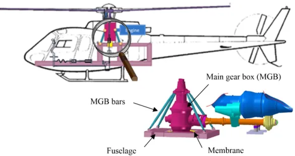
Therefore, its behavior depends on its dynamic characteristics and the filtering systems placed between the rotor and the fuselage (as shown in Fig. 1). In this sequel, we will focus on one of these filtering systems: the SARIB system (called Suspension Antivibratoire à Résonateur Intégré dans les Barres in French).
1 http://www.20sim.com/
Overview of the MGB-Fuselage suspensions 3
Fig. 1 - Helicopter suspension between the MGB and the aircraft structure
2.2 Interest and functions
The MGB-Fuselage suspension must ensure several important functions. Firstly, the joint allows the transmis-sion of the static force necessary to the sustentation of the helicopter with a limited static displacement. Moreover, the suspension helps to reduce the mechanical vibrations transmitted to the fuselage according to the force and displacement aspects. In this paper, we will focus on this latter function.
2.3 Operating principle
The classical MGB-Fuselage suspension is composed of four MGB bars and a main membrane as shown in Fig. 2a. The MGB bars can rigidly suspend the fuselage without flexibility to the rotor and thus transmit the lift from the rotor to the structure.
The membrane is a flexible suspension with the following observed behavior:
- a low stiffness for angular movements around the roll and pitch axes and the linear vertical pumping displace-ment,
- a very high stiffness for linear movements perpendicular to the vertical direction and for the yaw movement. Thus, the membrane allows the angular movement of the MGB around the pitch and roll axes. The flexibility of the membrane around these axes allows a strong filtration of the dynamic moments around these axes. In addi-tion, the membrane transmits the main rotor torque thanks to its very high stiffness around the yaw axis. In con-clusion, the conventional suspensions allow filtering pitch and roll dynamic moments without filtering the pump-ing dynamic efforts.
(a) (b)
The suspension equipped with SARIB system is a vibration absorber. Its purpose is to render the filtering of these pumping dynamic efforts possible. On the SARIB solution, beaters with flapping masses are added between the MGB bars and the fuselage Fig. 2b. They permit a vertical degree of freedom to the MGB with regard to the fuselage. The principle of the SARIB system is to tune, for an accurate defined frequency, these flapping masses on each SARIB bar so as to create inertial forces on the fuselage opposite to the force of the MGB bars on the beaters. The equilibrium of a SARIB bar enables to better understand this principle. In other words, there is an anti-resonance phenomenon on the transmissibility function between the excitation applied to the MGB. Hence, the forces transmitted to the fuselage can be strongly reduced at this anti-resonance frequency.
In the semi-active suspension, the flapping masses on the beaters can be translated and be consequently called tuning masses. The idea of the semi-active suspension will be to tune the positions of the moving masses so that the anti-resonance frequency of the structure corresponds to the frequency of the excitation forces on the MGB.
2.4 Overview of the experimental setup
According to helicopters engineers, two types of experiments can be conducted in order to test the flight be-havior of the MGB-fuselage system: either directly on a helicopter or on an experimental setup. The first type of test is more expensive and is carried out mainly in the validation phase of the system. The research work presented in this paper is focused on the pre-sizing phase.
It was thus decided to develop an experimental setup on a small scale so as to conduct the experimental tests. The geometry and mass properties correspond to a light helicopter with a scale of approximately ½ (see appendix). The models proposed in this paper have been simulated with the data of this experimental setup. This experimental setup preserves the 3D feature of the real system by the use of four MGB bars. It allows the simulation of a semi-active system with SARIB beaters equipped with tuning masses. The experimental setup has to represent the flight behavior of the helicopter in different operating phases: hover, up / down or turn. In these operating phases, the MGB is subjected to pumping, pitch and roll excitements. On the experimental setup, the rotor action, provided by the aerodynamic forces and the blades stiffness, applied to the MGB will be approximated by a sinusoidal excitation at the frequency bΩ obtained with a vibration equipment.
Modeling and simulation framework 5
3
Modeling and simulation framework
3.1 Classical bond graph modeling
3.1.1 Brief reviewThe concept of energy is fundamental in the description of the evolution of technological systems. Energy is present in all areas of physics and is the link between them. From this observation, a number of tools with energetic representations for modeling complex systems have been defined. One of the main tools is the bond graph. The bond graph was created by H. Paynter [4] in 1959 and developed by R. Rosenberg and D. Karnopp [14] in the United States.
The bond graph is based on a study of the transfer of power in a system modeled by lumped parameters. The bond graph is a graphical modeling tool that covers all physical systems (mechanical, hydraulic, electronic, ther-mal...) regardless of their condition (linear, nonlinear, continuous …). It is represented as an oriented graph show-ing dynamic variables and power bonds between these variables. The bond graph systematically associates two different variables for each bond: a generalized effort variable (which is a force or a torque in mechanics) and a generalized flow variable (which is a translational or rotational velocity in mechanics) on each side of the half-arrow link. Each bond has therefore power information, obtained by the product of these two variables, and allows direct access to the energy transferred by a simple integration of power. The bond graph approach enables thus, the representation of mechatronic systems in a graphical form that describes the exchange of power between basic elements like inertia, compliance, dissipation, conservative power transformation, gyrator actions and sources.
More details on bond graphs can be found in [5, 6] on the basis, the operation and the construction of classical bond graphs. The classical bond graphs mentioned in this paragraph 3.1 also called 1D bond graphs deals with mechatronics system with elementary motions (translation and rotation around fixed axis) and without 3D move-ment.
3.1.2 Benefits of bond graphs
The major benefits of bond graphs developed mainly in [5] [6] are well-known in mechatronics communities. They are thus only recalled here but not detailed for space reasons. As mentioned previously, the bond graph is a unified and energetic language covering almost all physical domains. The bond graph facilitates a systemic ap-proach necessary to design a mechatronic system thanks to its features as graphical display, object-oriented lan-guage and acausality (in a similar manner as Modelica [15]).
In addition, bond graphs also enable the use of new features such as structural analysis [16] of a system from the bond graph structure (causality, controllability, observability, inversibility, etc). While these characteristics is not utilized in this paper, the exploitation of bond graphs is mentioned here since it constitutes of a perspective of this work.
3.2 Modeling of multibodies system with bond graphs
3.2.1 Brief reviewThe aim of this section is to recall the main contributors concerning methodologies for modeling the dynamics of three-dimensional multibody systems (MBS). More detailed reviews specifying applications of BG modeling for MBS can be found in [5], [6] and [17].
The first bond graph models of multibody systems have been proposed by D.C Karnopp and R.C Rosenberg [18, 19] thanks to an analytical approach based on an appropriated choice of generalised coordinates, the construc-tion of juncconstruc-tion structure for the formulaconstruc-tion of the kinematic laws and a lagrangian formulaconstruc-tion.
In the 90’s, thanks to the multibond graph (MBG) formalism [20] [21] (an extension of bond graphs where the scalar power bonds become vector bonds and the elements multiports), the application fields of the bond graph were extended to the study of multibody systems with three dimensional movements.
The bond graph approach used for multibody systems was introduced by A. M. Bos [7, 8]. In his PhD, he developed bond-graph models for three-dimensional multibody systems and discussed how to derive the equations of motion from the bond-graph in several different forms. At this time, although he managed to conduct simula-tions of a 3D motorcycle, the equasimula-tions had been derived with a manual process.
Library models for a rigid body and for various types of joints have been provided in [10] so that bond graph models of rigid multibody systems can be assembled in a systematic manner.
J. Felez [22] developed a software that helps with modeling multibody systems using bond graphs. To handle derivative causalities with this software, he proposes a way to introduce Lagrange multipliers into the system so as to eliminate derivative causality.
In [23, 24], different methods for simulating BG models have been presented. Simulations have been conducted with a predecessor of 20-sim software and numerically compared mainly on the computing time and accuracy. Even if the possibility of using multibond graph was evocated, the difficulty of implementing bond graphs with vector bonds were not mentioned.
Furthermore, W. Marquis-Favre and S. Scavarda [25] propose a method to simplify bond graph models for multibody systems with kinematic loops. Nevertheless, few complex multibody systems with kinematic closed loops have been simulated.
3.2.2 Discussion on the use of bond graphs for multibody systems
In [6], [26], some difficulties in using bond graphs for multidomain applications namely multibody systems have been pointed out. Even if some of these difficulties such as ( the use of frame-dependent vectors and gener-ation of constraints at velocity level) are persistent, other points described hereafter have been improved or solved thanks to the evolution of dedicated software for bond graphs and the use of appropriated methods.
Firstly, the multibond graph allows to simplify the bonds between the bond graph elements and the readiness of the model. Nevertheless, the causality analysis of multibond graphs can be considered as a difficult task as mentioned in [6]. Multibond graphs do lead to causality constraints as mentioned in [27] and [28]: 1) each dimen-sion of a vector bond must have the same causality, 2) the causality of transformers implied in cross product and the causality of gyrators is imposed. However, some methods for dealing with these two constraints (namely sin-gular perturbations or Lagrange multipliers, …) have been proposed [27] and are efficient to resolve these diffi-culties.
Secondly, thanks to the use of the word bond graph (WBG), the multilevel representation is permitted and allows for the concatenation of the bond graphs’ bodies and joints. This technique makes it possible to "zoom in / out" on different parts of the system, such as in a Simulink model. However, with bond graphs, the hierarchical decomposition is not made in mathematical functions as in block diagrams but in models of subsystems. As defined in [5], the structural models are defined as an assembly of models of physical elements or subsystems following the same architecture as the real system without prior analysis on how to connect the various subsystems. From the authors’ points of view, bond graphs thus belong to this class of structural modeling tools. As a consequence, it is possible to obtain a global representation of the system built from subsystems which facilitates the manage-ment of interactions and/or couplings.
Thirdly, the modularity allowed by the bond graph method enables the model to evolve and meet the levels of complexity required for each design problem by the addition or modification of new components and subsystems and by replacing behavior laws.
Fourthly, even if it is true that bond graphs for multibody systems require a certain level of expertise, the generation of equations from the bond graph models can be done automatically by dedicated softwares to bond graphs such as 20-sim and even for complex bond graph models as it will be shown in this paper through the MGB-Fuselage suspension. Naturally, it is important to note that methods such as the singular perturbation method used in this paper must be used to tackle constraints due to vector bonds and derivative causalities which can appear on some inertial elements.
3.2.3 Approach chosen : the BOS and Tiernego method
In order to keep a modular approach, the principal method for modeling multibody system with bond graphs is the Bos and Tiernego method [7]. This method enables a multibody system to be built as an assembly of bodies and joints. The principle of this method is based on the use of absolute coordinates systems and Newton-Euler equations. Indeed, in such a way, the dynamic equations of a rigid body depend on, obviously, his mass/inertia parameters and also on geometric parameters defined only for the considered body. Consequently, the dynamic equations of the complete system consist of a sum of the dynamic equations of each body depending only on its own parameters.
Modeling and simulation framework 7
3.3 MBG modeling of closed kinematic chains (CKC)
3.3.1 Problem statementThe simulation of mechanical systems with kinematic loops requires specific methods. This difficulty does not come from the bond graph tool but from the application of dynamics equations to such systems where some kine-matic variables are linked together because of the kinekine-matic constraints. Regardless the analytical method em-ployed (fundamental principle of dynamics or Lagrange equations with multipliers), when no preliminary kine-matic works is done, the equations obtained are differential algebraic equations (DAEs) whose numerical resolution requires specific numerical integration methods. In bond graphs, this class of constrained mechanical systems that leads to differential-algebraic equations present inertial elements with derivative causality whose variables are dependent on others variables considered as independent through algebraic constraints.
In this paper, in order to keep a modular approach as mentioned in the previous section, absolute coordinates are selected. Consequently, in this case (absolute coordinates selected), it is important to notice that open chain (OC) and closed kinematic chain (CKC) systems both lead to a DAE formulation. Consequently, one of the nec-essary priorities of the simulation method exposed in this paper will be to handle DAEs.
3.3.2 Resolution methods
These difficulties to solve numerically differential equations are developed, for example, in W. Marquis-Favre [29]. A recent and concise review of the methods for solving DAEs can be also found in [30]. To sum up, one can find three groups of methods: the direct resolution of the DAE thanks to specific solvers, the reduction of the DAE in an ODE like the coordinates partitioning method or minimal coordinates and the conversion to an ODE by modifying the model system. The singular perturbation method which is used in the paper belongs to the last category of these methods that is to say the conversion to an ODE by modifying the model system.
3.3.3 Approach chosen : the singular perturbation method
The bond graph simulation with the singular perturbation method is quite easy to implement compared to conventional techniques used during an analytical study. We thus decided to use the method of singular perturba-tion which, from our point of view, keeps a physical insight and permits to keep a modular approach without the need to use additional stabilization techniques to circumvent the drift of the constraints.
The singular perturbation method consists in augmenting the bond graph of the joints with parasitic elements [31] [32] also called virtuals springs in [12]: stiffness and damping elements corresponding to C energy store element and R resistive element.
The enforcement of constraints through parasitic C and R elements instead of using ideal flow sources can circumvent the two multibond constraints mentioned in 3.2.2 thanks to the effort-out causality permitted by the parasitic elements. Firstly, it allows the same causality assignments for all the bonds of a multibond. Secondly, it allows to suppress the causality conflict which may appear because of the imposed causality of the transformers implied in the cross product and gyrators [27].
If the kinematic constraints modeled by the bond graph where the joints are rigidly imposed, derivative cau-sality appears at the multibonds connected to the translational inertia elements. The derivative caucau-sality, due to constraints, requires that the equations derived from the bond graphs to be differential algebraic equations (DAEs). The resolution of such equations is quite complex from a computational point of view as we explained before. The singular perturbation method relaxes the kinematic joint constraints. The dynamic equations are in an ODE form with no geometric constraints to deal with. It leads thus to a bond graph with integral causality which can be simulated easily using explicit solvers.
The values of the compliant elements must be chosen carefully. To our knowledge, two methods for selecting these elements exist : 1) the eigenvalues decoupling between the parasitic frequency and the system frequency, 2) the use of activity metric [31]. These parameters can be chosen so as to model the joint compliances which exist in all mechanical joints. Thus, this point gives to this method a physical significance. The stiffnesses introduced should be high enough so as not to change the dynamic of the system but not too high so as to prevent the numerical difficulties of stiff problems (with high-frequency dynamics). This method leads to a necessary compromise be-tween the accuracy of the results and the simulation time: the stiffer the system is, the more numerical errors are reduced but the more simulation time remains important. However, the increase of the simulation time can be balanced by parallel processing as the mass matrix in a block-diagonal form can enable to decouple the system as
it is explained in [12]. As T. Rayman recommends, adding a damping element (R resistive element) in parallel with the stiff spring (C energy store element) enables to dampening of the high eigen frequency associated with the high stiffness. The exact influence of these parameters still remains a research work in which the authors are particularly interested in.
4
Modeling of the passive suspension
The bond graph modelling steps described above will now be applied to model the MGB-fuselage suspension equipped the with SARIB device. First, the mechanical model of the MGB-fuselage suspension and the associated assumptions will be presented. Secondly, the construction of the bond graph model of the MGB-fuselage suspen-sion will be detailed.
4.1 Modeling assumptions of the MGB-Fuselage suspension
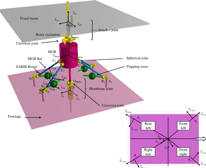
The 3D MGB-fuselage suspension with free fuselage is a set of 14 rigid bodies (the MGB, four MGB bars, four SARIB beaters, four intermediate bodies and the fuselage) and includes eighteen kinematic links (four revo-lute joints, eight spherical joints and two prismatic joints). The kinematic scheme of the 3D MGB-fuselage sus-pension is shown in Fig. 4.
Fig. 4 - Kinematic scheme of the 3D joint between the main gearbox and the fuselage C2 C1 C3 Spherical joint SARIB Beater B2 B1 B3 A1 A2 A3 F z F y F x MGB x MGB y FF y FF x FF z Rotor excitation SB x MB z MB x MB y SB y SB z MGB Fixed frame Fuselage Universal joint Universal joint AMGB OMGB MGB Bar MGB z GF Flapping mass GMGB GSB GMB OFF OF 2 F int x 1 F a F y F x 3 F int y 3 F int x 3 A 2 F int y 2 A 1 A 4 A 1 F int y 1 F int x 4 F int x 4 F int y Rear left Front left Front right Right rear « Attach » joint Membrane joint
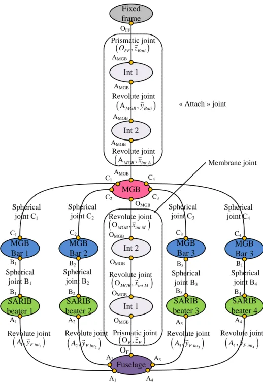
Modeling of the passive suspension 9 For the sake of clarity, the different kinematic joints are also described in the joints graph Fig. 5.
Fig. 5 - Joints graph of the 3D SARIB passive suspensions
The MGB is suspended by a joint called “attach” to the fixed frame. This joint consists of a universal joint and a prismatic joint. The weight of the system (mainly the weight of the MGB and the fuselage) is taken up by a tension spring at the prismatic joint of this attach. The spring is dimensioned such that the natural frequency of the mass / spring system is small enough and distant from the excitation frequency applied to the MGB.
The structure of the suspension consists of four identical legs and a central membrane. Each leg consists of SARIB beaters and a MGB Bar connected by a spherical joint. The upper ends of these legs are connected to the MGB with spherical joints and the lower ends of these legs are connected to the fuselage through revolute joints. The revolute joints between SARIB beaters and the fuselage have a torsion spring dimensioned such that the antiresonance frequency in the efforts transmitted to the fuselage is positioned on the rotor excitation frequency while taking up enough the effort to lift the helicopter with a small displacement between the MGB and fuselage.
MGB
Bar 1
MGB
SARIB
beater 1
Fuselage
MGB
Bar 2
SARIB
beater 2
MGB
Bar 3
SARIB
beater 3
MGB
Bar 3
SARIB
beater 4
Int 2
Int 1
Spherical joint B1Revolute joint Prismatic joint
Revolute joint Spherical joint C1
Fixed
frame
Int 2
Int 1
Prismatic joint(
A y1, F int1)
C1 Revolute joint(
AMGB,yBati)
C2 C3 C4 AMGB AMGB OFFO
F OMGB OMGB OMGB OMGB Revolute joint(
OMGB,xint M)
OMGB C1 AMGB AMGB B1 B1 A1 A1 A2 A4 A3 Revolute joint(
A y2, F int2)
Spherical joint C2 Revolute joint(
AMGB,xint A)
(
OFF,zBati)
AMGB C2 B2 Spherical joint B2 Spherical joint C3 Spherical joint C4 Spherical joint B3 Spherical joint B4 B2 A2 B3 A3 B4 A4 C3 B3 C4 B1 Revolute joint(
A y3, F int3)
Revolute joint(
)
4 4, F int A y(
OMGB,xint M)
(
O ,F zF)
« Attach » joint Membrane jointGiven the physical phenomena observed, the main membrane between the MGB and the fuselage is modeled by two revolute joints with orthogonal axes (also called universal joint) and a prismatic joint in serial. The flexi-bilities of the membrane in pumping, roll, and pitch are modeled by the degrees of freedom of these joints com-bined with stiffness. A torsion spring with low stiffness at each revolute joint of the universal joint and a linear spring, also with low stiffness along the z-axis will model the filtering carried out by the membrane. The rigidities of the membrane are modeled by rigid joints or, in other words, by a lack of degree of freedom around or along the movements considered.
These bodies are assumed to be rigid. The intermediate parts (called Int1 and Int2) are supposed with negligible masses. As previously mentioned, absolute coordinates have been chosen for modularity reasons. Some local mov-ing reference frames are attached to these bodies:
(
, , ,)
FF FF FF FF FF
R = O x y z attached to the fixed frame,
(
, , ,)
MGB MGB MGB MGB MGB
R = G x y z attached to the MGB,
(
, , ,)
SB SB SB SB SB
R = G x y z attached to the SARIB Beaters,
(
, , ,)
MB MB MB MB MB
R = G x y z attached to the MGB Bar,
(
, , ,)
F F F F F
R = G x y z attached to the fuselage and RFinti =
(
A xi, Finti,yFinti,zFinti)
also attached to fuselage so as to
facilitate the definition of the axis of the revolute joints.
4.2 Modeling assumptions of the suspension environment
As previously mentioned in section 1, the action of the rotor on the MGB in the experimental setup is approxi-mated by a sinusoidal excitation with a frequency bΩ.
The external mechanical actions applied to the MGB are the forces applied by the vibrating shakers. The de-scription of the experimental setup shall be specified in Section 5.2 of this paper. These excitations will be applied along or around the joints of the “attach” joint between the fixed frame and the MGB. They allow the MGB to be subjected to pumping, pitch and roll excitations. These mechanical actions will only consist of a dynamic compo-nent to analyse the vibration behaviour of the suspension.
For the pumping excitation, the wrench applied by the actuator at the mobility of the prismatic joint is:
(
)
( )
( )
( )
0 Bati Bati O f t zactuator along vertical axis prismatic joint avec f t F g t
τ → = = ×
(1)
For roll excitation, the wrench applied by the actuator at the mobility of the revolute joint around roll axis is:
(
)
( )
0( )
( )
BTP
r r Bâti
A
Actuator around roll axis roll revolute joint avec m t M g t
m t y τ → = = × (2)
For pitch excitation, the wrench applied by the actuator at the mobility of the revolute joint around pitch axis is:
(
)
( )
0( )
( )
BTP p p int A Aactuator around pitch axis pitch revolute joint avec m t M g t
m t x τ → = = × (3)
Different types of excitation are used by modulating the amplitude of each excitation by a dimensionless function g(t): constant, sinus type or swept sine. The constant excitation permits to ensure that the equilibrium position of the system under its own weight is physically acceptable. The sine excitation permits to get more accurate frequencies of the anti-resonance frequencies.
The swept sine excitation is used to analyze the frequency behaviour of the system including resonances and anti-resonances frequencies.
For the swept sine excitation, a modulation function was constructed, as shown in four parts:
- within [0, t1], a progressive increase to a sinusoidal excitation at a frequency of
f
start de 5Hz is carried outwith a linear amplitude variation,
( )
(
)
( )
(
)
2 1 2 1 2 1 1 1 1 2 1 1 0, , 4 sin 2 2 2 2 1 , , sin 2 2 2 2 start start t t t g t t t t t t t t g t t t t t tω
ω
∀ ∈ = ∀ ∈ = − − + − + (4)Modeling of the passive suspension 11 - within [t1, t2], the sine excited mode at
f
startis preserved the necessary time so that the transient modedisappears and there is only permanent regime,
[ ]
1, 2 ,( )
sin(
start)
t t t g t ω t
∀ ∈ = (5)
- within [t2, t3], a linear swept sine is used with a sweep frequency from
f
start (5Hz) tof
end (25Hz). Theexpression of the chirp signal is given in [33] and recalled below :
[ ]
2,
3,
( )
sin
(
2) (
2)
2
startt
t t
g t
t t
t t
T
ω
ω
∆
∀ ∈
=
+
−
× −
∆
(6)With ∆ =ω ωend −ωstart and ∆ = −T t3 t2
- within [t3,+], the sine excited mode at
2 end end f ω π = (25Hz) is kept.
[
3,]
,( )
sin(
end)
t t g t ω t ∀ ∈ +∞ = (7)For the conducted simulations, the time intervals were defined with the numerical following values: t1=3s, t2=5s and t3=25s.
Fig. 6 - Modulation function of the excitation g(t)
4.3 Construction of the bond graph model of the MGB-Fuselage joint
4.3.1 Components modelingThe components modelling (rigid bodies and kinematic joints) of the system will be now be presented.
4.3.1.1 Rigid bodies
A reminder of the general rigid body modelling
Let us remember the architecture of a rigid body multibond graph model based on [5], [8], [25], [34]. This bond graph architecture is based on the Newton-Euler equations with the inertia matrix (modeled with a multiport energy store element
i i
S ,G i
I in the upper part) associated with gyroscopic terms respectively (modeled with a multiport gyrator element also called Eulerian Junction Structure about mass-center of body i expressed in its frame
i
G i
EJS and the mass matrix modeled with a multiport energy store element
[ ]
i 0m in the lower part). The upper part of the bond graph represents the rotational dynamic part expressed in the body frame while the lower part is for the translational dynamic part expressed in the inertial reference frame (or Galilean frame). The two corresponding 1-junctions arrays correspond respectively to the angular velocity vector of body i Ω
( )
i/ 0 iand the translational velocity vector of the center of mass of body i V G(
i/R0)
0expressed in these two coordinate frames.The central part of the MBG describes the kinematic relations between the velocities of the two points of the body i (V M
(
j /R0)
iand V M(
k /R0)
0) and the velocity of the center of mass V G(
i/R0)
iresulting from the for-mula of the rigid body.0 5 10 15 20 25 30 time {s} -2 -1 0 1
o ct o de odu at o de a p tude de e c tat o
( )
g t
[s]
t
Progressive increase
of magnitude Sweep frequency
Excited mode at 5Hz Excited mode at 25 Hz
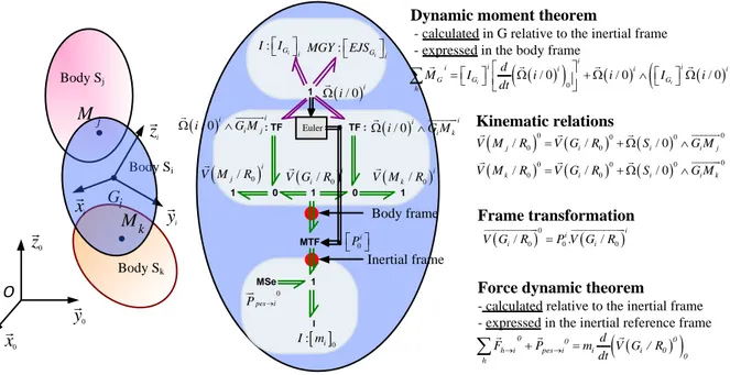
Fig. 7 - Bond graph model of the rigid body
As the translational dynamic is expressed in the inertial reference frame, a modulated transformation element (MTF) between V G
(
i /R0)
iand V G(
i/R0)
0permits the coordinate transformation between the body frame and the inertial frame. The rotation matrix can be calculated from Euler angles. In this paper, the XYZ Cardan angles have been employed. The angular velocity components of the considered body expressed in the body frame (called the pseudo-velocities or Euler angles rates of changes) are used to determine the body’s orientation and the corre-sponding coordinate transformation matrix. This classical process is reminded in Fig. 8. It should be noted that the initial conditions used for the integration of time derivatives of the Euler angles must be consistent in regards to the kinematic constraints.Fig. 8 - Calculation of the Euler angles and rotation matrix from the angular velocity
The MGB
The MBG representation of the construction is given in Fig. 9. The bond graph representation shows as many branches in the structure junctions as kinematic joints for the determination of the velocities of corresponding points. From the linear velocity of the center of mass GMGB and the instant rotation velocity Ω
(
MGB/ Fixed frame)
, the linear velocity of the point OMGB, the linear velocity of AMGB point of the MGB and the linear velocities Ci point at the ball joints between BTP and BTP bars are calculated.
0 0 1 : TF TF : MSe 1 1 1 1 I MTF : i G i I I : i G i MGY EJS ( )i/ 0i Ω ( / 0) i i V G R V M( k/R0)i
(
/ 0)
i j V M R ( )i/ 0i G Mi ki Ω ∧ ( )i/ 0i G Mi ji Ω ∧ 0 i P [ ]
0 : i I m 0 pes i P → Inertial frame Body frameDynamic moment theorem
- calculated in G relative to the inertial frame - expressed in the body frame
( )
(
)
( )(
( ))
0 / 0 / 0 / 0 i i i i i i i i i G G G h d M I i i I i dt = Ω + Ω ∧ Ω ∑
Kinematic relations(
)
( ) ( ) ( ) ( ) ( ) 0 0 0 0 0 0 0 0 0 0 0 0 / / / 0 / / / 0 j i i i j k i i i k V M R V G R S G M V M R V G R S G M = + Ω ∧ = + Ω ∧ Force dynamic theorem
- calculated relative to the inertial frame - expressed in the inertial reference frame
( )
(
)
0 0 0 h i pes i i i 0 0 h d F P m V G / R dt → + → =∑
Frame transformation ( )0 ( ) 0 0 0 / i. / i i i V G R =P V G R 0y
0z
O jM
i G Body Sj Body Si Body Sk 0x
iz
iy
kM
ix
Euler Initial conditions(
/ 0)
x i i y z B Ω Ω = Ω Ω ( )
( )
( )
( )
( )
( )
( ) ( )
( ) ( )
(
)
cos tan sin tan
sin
cos tan sin tan
/ 0 / / 0 cos 0 1 i i x y z B ε α γ γ β γ γ γ γ γ β β β β Ω Ω = Ω Ω − − α ε β γ = α ε β γ = ε=
∫
εdu+εini Calculation of pseudo-velocities Intégration Rotation matrix 0cos( ) cos( ) cos( )sin( ) sin( )
cos( )sin( )sin( ) cos( )sin( ) cos( ) cos( ) sin( ) sin( )sin( ) cos( )sin( ) sin( )sin( ) cos( ) cos( )sin( ) cos( )sin( ) cos( ) sin( )sin( )) cos( ) cos( )
i P β γ β γ β γ α β α γ α γ α β γ β α α γ α γ β γ α α β γ α β − + − − = + − ini ini ini ini α ε β γ = Euler 0 i P
(
Bi/ 0)
i ΩModeling of the passive suspension 13
Fig. 9 - Bond graph modeling of the MGB with its environment
The fuselage
With a similar approach, the bond graph modelling of the fuselage is given in Fig. 10.
Fig. 10 - Bond graph model of the fuselage with its environment (MGB/ 0)MGB Ω ( 1 / 0) MGB V C ∈MGB MTF 1 1 1 1 1 1 1 1 MSe Weight TF TF TF TF TF TF 1 0 0 0 0 0 0 ( 2 / 0) MGB V C ∈MGB ( 3 / 0) MGB V C ∈MGB ( 4 / 0) MGB V C ∈MGB 1 MGB MGB GC 2 MGB MGB G C MGB MGB MGB G O IntA 2 Revolute joint Spherical joint MGB bar 1 Revolute joint IntM 2 4 MGB MGB GC MGB MGB MGB G A ( BTP / 0)MGB V O ∈MGB V G( MGB∈MGB/ 0)MGB ( )0 / 0 MGB V G ∈MGB 0 MGB P [ ]0 : MGB I m : GMGB MGB I I : MGB G MGB MGY EJS 3 MGB MGB GC Spherical joint MGB bar 2 Spherical joint MGB bar 2 Spherical joint MGB bar 4 Euler Rotational dynamics Translational dynamics MTF 1 1 1 1 1 1 1 MSe TF TF TF TF TF 1 0 0 0 0 0 Spherical joint SARIB beater 1 SARIB beater 2 SARIB beater 3 SARIB beater 4 IntM 1 Prismatic joint
Rotational dynamics
Translational dynamics
(
Fus/ 0)
Fus Ω Weight 1 Fus Fus G A (
1 / 0)
Fus V A ∈Fus(
Fus / 0)
Fus V G ∈Fus[
]
0 : Fus I m : Fus G Fus I I : Fus G Fus MGY EJS 2 Fus FusGA GFusOFusFus
3 Fus Fus GA 4 Fus Fus G A
(
)
0 / 0 Fus V G ∈Fus(
2 / 0)
FusV A ∈Fus V A
(
3∈Fus/ 0)
Fus V A(
4∈Fus/ 0)
Fus0 Fus P Euler Spherical joint Spherical joint Spherical joint
The SARIB beaters
The bond graph model of a SARIB beater kinematically linked to the fuselage and the MGB bars is given in Fig. 11.
Fig. 11 - Bond graph model of a SARIB beater i kinematically linked to its environment
The MGB bars
The bond graph model of a MGB bar beater kinematically linked to the MGB and a SARIB bar is given in Fig. 12.
Fig. 12 - Bond graph model of MGB bar i kinematically linked to its environment
MTF 1 1 1 1 MSe Weight TF TF 1 0 0 0 BSi P
(
BS / 0i)
i BS Ω BSi BSi i G B (
i / 0)
BSi V A ∈BSi(
/ 0)
BSi BSi i V G ∈BS(
)
0 / 0 BSi V G ∈BSi[
]
0 : BSi I m : GBSiBSiI I MGY: EJSGBSiBSi
(
i / 0)
BSi V B ∈BSi BSi BSi i G A Fuselage MGB bar i Spherical joint Revolute joint Euler MTF 1 1 1 1 MSe TF TF 1 0 0 Spherical joint SARIB beater i(
BBi/ 0)
BBi Ω Weight BBi BBi i G C (
i / 0)
BBi V C ∈BBi(
BBi / 0)
BBi V G ∈BBi(
)
0 / 0 BBi V G ∈BBi[
]
0 : BBi I m : BBi G BBi I I : BBi G BBi MGY EJS(
i / 0)
BBi V B ∈BBi BBi BBi i GB 0 BBi P MGB Spherical joint Rotational dynamics Translational dynamics EulerModeling of the passive suspension 15
4.3.1.2 Kinematic joints
The joint modelling will now be detailed. The singular perturbation method is here implemented by the addition of parasitic elements which were presented in the previous section. The joint models permit the expression of the constraints that are introduced when rigid bodies are connected. As the bond graph model of the rigid body, the joint models have been built in a modular way in the sense that they have links with rigid bodies and their modelling does not change when the whole model of the system is assembled.
The revolute joints
Eight revolute joints are present in the system: two for the universal joint in the attach joint between the fixed frame and the MGB, two for the universal joint in the membrane between the MGB and the fuselage, and four between each SARIB beaters and the fuselage. The bond graph modelling between the SARIB beaters and the fuselage is given in Fig. 13. The bond graph models of the other revolute joints are designed in a similar manner.
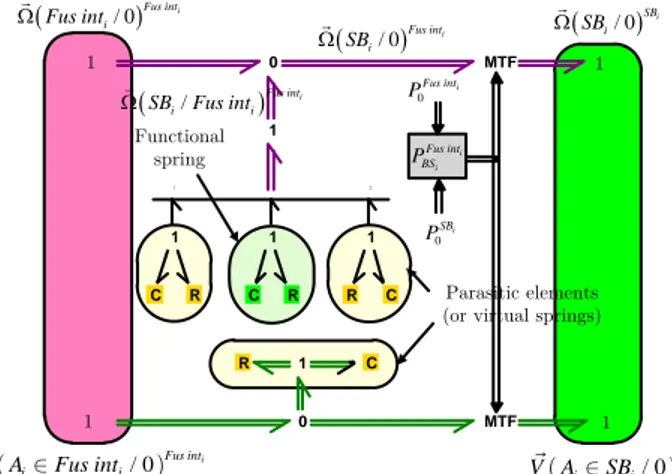
Fig. 13 - Bond graph model of the revolute joint between the SARIB beaters and the fuselage
The upper part of this joint’s model corresponds to the angular velocities. The lower part of this joint’s model corresponds to the translational velocities. The R/C elements in this model are functionally different. On the one hand, the R/C elements corresponding to the stiffness and damping around the y axis (revolute joint’s axis) model the behaviour of the torsional spring. On the other hand, the R/C elements with high stiffness and some damping around the other axes model the virtual springs since there are no physical springs in these directions. They permit to block the degree of freedom along and around these axes and make the numerical simulation possible (as ex-plained in section 3).
The spherical joints
Eight spherical joints are present in the system: four between the SARIB beaters and the MGB bars and also four between the MGB bars and the MGB. The bond graph modelling of the spherical joint between the SARIB beater and a MGB Bar is described in Fig. 14. The latter shows the blocking of the translational degree of freedom in which the relative translational velocities are close to zero thanks to the virtual springs. The other spherical joints are built in the same manner.
Fig. 14 - Bond graph model of the spherical joint between a MGB bar i and a SARIB beater i C C C C MTF MTF 1 1 1 1 3 1 2 R R R R 1 0 0 ( / 0)SBi i SB Ω ( / 0)Fus inti i Fus int Ω 1 ( / 0) i Fus int i SB Ω ( / )Fus inti i i SB Fus int Ω / 0Fus inti i i V A Fus int / 0SBi i i V A SB Parasitic elements (or virtual springs)
i i Fus int BS P 1 1 Functional spring 1 0 i Fus int P 0 i SB P
(
/ 0)
RSBi i SB Ω(
/ 0)
BSi R i i V B ∈BS R(
/ 0)
RMBi i MB Ω(
/ 0)
MBi R i i V B ∈MB R i i BS MB P(
/)
RSBi i i MB SB Ω MTF MTF 1 R R 1 0 0 1 1 1 1 C Parasitic elements Functional spring 0 i BS P 0 i MB PThe prismatic joints
The bond graph model of the prismatic joint between the MGB and an intermediate body is given in Fig. 15.
Fig. 15 - Bond graph model of the prismatic joint between the MGB and a intermediate body
4.3.2 Excitation models
The mechanical actions developed by the actuators are modelled by an effort source connected to the junctions
1 which are free in the attach joint. The example of the implementation of an excitation by a swept sine at the pitch
joint is shown in Fig. 16.
Fig. 16 - Bond graph model of the actuators of the excitation
Depending on the selected excitation direction (pumping, roll or pitch), this source will be respectively con-nected either to the free junction of the prismatic joint, or the revolute joints around the roll or pitch axis. Three choices of excitation forms may also be selected: constant for a natural mode excitation (if this constant is zero) or a static study, sinusoidal or swept sine for excited modes.
The practical realization of these actuators will be conducted using vibration shakers as we will detail in the experimental validation section.
4.3.3 Assembly 0 0 ò R R R 3 2 1 1 1 1 1 1 1 MTF C C C C
(
/ 0)
Fus Fus V O ∈Fus R(
/ 0)
Fus Fus R Ω(
)
0 / Fus INT R Ω(
/ 0)
Fus MGB V O ∈INT R(
/ 0)
Fus MGB Fus Fus R O O Ω ∧(
MGB /)
Fus V O ∈MGB Fus Parasitic elements (or virtual springs)Functional spring 1 1 1 1 Excitation Fixed frame MGB Prismatic joint Revolute joint Revolute joint Chirp signal Direction: Form : Constant Sine Pitch Sweep 1 1 1 MotionProfile Se Se Se Pumping Roll
Modeling of the passive suspension 17 These rigid bodies and joints models, as described above, are then connected together according to the archi-tecture defined in the kinematic diagram. The bond graph model of the 3D MGB-fuselage suspension is given below in Fig. 17. As expected, the structural aspect of the model is explicit in so far as the structure of the model is similar to the joints graph of the system.
Fig. 17 Bond graph model of the passive MGB-fuselage suspension
4.3.4 Simulation protocol Getting equations
The step of generating the mechanical equations is fully automated and transparent to the user using the 20-sim software. In this step, the solver reads data corresponding to the bond graph model and builds a mathematical problem: the equations of the system.
Resolution of the equations
The used bond graph software (20-sim) then solves the equations. With the method of singular perturbation, this step resolution can be performed simply using classical integration schemes for solving differential equations ODE solver such as Runge Kutta 4 (RK4). However, the integration scheme that has been used is the Backward
MGB Fuselage Glissière MB1 1 R MB 0 R /R SB1 1 R SB 0 R /R SB1 1 R SB 0 R /R RFus 1 0 A Fus/R V R1 1 1 0 A /R SB V SB R1 1 1 0 B /R SB V SB R 1 1 1 0 B /R MB V MB R 1 1 1 0 C /R MB V MB R 0 C1 /R MGB V MGB RFus Fus 0 V O Fus/R RFus Fus 0 R /R Rint int 0 R /R RMGB MGB 0 V O MGB /R RFus Fus 0 R /R RMGB MGB 0 R /R MB1 1 R MB 0 R /R RMGB MGB 0 R /R RFus Fus 0 R /R IntA 1 IntA 2 IntM 2 IntM 1 Excitation Fixed frame Prismatic joint Revolute joint Revolute joint MGB bar 1 MGB bar 2 MGB bar 3 MGB bar 4 SARIB beater 1 SARIB beater 2 SARIB beater 4 SARIB beater 3 Spherical joint Spherical joint Spherical joint Spherical joint Spherical joint Spherical joint Spherical joint Spherical joint Revolute joint Revolute joint Revolute joint Revolute joint Revolute joint Revolute joint Rint int 0 R /R RFus Fus 0 R /R
Differentiation Formula (BDF). It was preferred as it allows a simulation of a stiff problem which is much faster than explicit solvers (like RK4).
Post-processing
From the mathematical solution, the solver computes and communicates the results requested by the user. 20-sim allows the user to evaluate and easily plot any of the physical quantities involved in the bond graph model of the system. In addition, graphs can be exported to various types of image-formats or data with .csv or .xls file. The data exportation allows for the comparison of results from different sources in the same graphic interface (for example Matlab).
5
Simulation and validation of the passive suspension
5.1 Validation protocol
So as to validate the suspension’s model, a process based on two steps has been conducted.
The first step is a verification step by comparison of the simulation results with MapleSim software which contains a library dedicated to multibody systems.
The second step is a validation step by comparing the simulation results with those provided from the experi-mental setup. This step will be presented in future works since the electronic devices and the vibration equipment are not yet installed.
5.2 Complementary description of the experimental setup
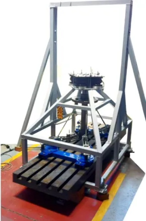
The experimental setup was performed by maintaining the architecture of a real device (Fig. 3). The corre-spondence between the different mechanical elements of a helicopter and the experimental setup will be detailed in this paragraph.
To reproduce the effects of the rotor lift, the set {BTP-link-fuselage} has been suspended from the fixed frame (Fig. 3). This joint has to lift up the entire weight suspended by analogy to the static force of lift, it was performed by the use of pneumatic components. They were designed so that the natural frequency induced by the overall stiffness is below 2Hz.
The fuselage was replaced by a rigid mass called fuselage mass (Fig. 3).
A single body has replaced the set {rotor shaft-MGB} and the rotation has been deleted. This single body is composed of a shaft equipped with a recessed tray (Fig 18).
Simulation and validation of the passive suspension 19 The overall joint between the fuselage mass and the system equivalent to the set {rotor shaft-MGB} has four bars, four semi-active SARIB beaters and a system representing the usually existing membrane on the helicopter.
The MGB bars consist of threaded rods that have a spherical joint without backlash at each end.
Each SARIB beater is linked by a revolute joint to the fuselage, which are themselves clamped to the fuselage mass as shown in Fig 18. Each SARIB beater is fitted with a moving mass (Fig.19) connected with a prismatic joint along the SARIB beater. The translational movement is controlled by means of a screw-nut system and a DC motor. It should be noted that, in this section, the moving masses are fixed on the SARIB beaters.
Fig.19 - Revolute joint between a SARIB beater and the fuselage
5.3 Use of MapleSim for BG model verification
The simulation parameters used for both the bond graph simulation and Maplesim simulation are summarized in the following table.
Table 1. Simulation comparison
Software MapleSim Bond graph conducted with 20-sim
Solver Rosenbrock (stiff) Backward Differentiation Formula (BDF)
Method Linear graph theory Singular perturbation
Number of coordinates 84 (14 bodies) 84 (14 bodies)
Number of constraints
74
(8 spherical joints, 8 revolute joints, 2 prismatic joints)
0
DoF 10 (6 + 4) 84
5.4 Comparison between simulation numerical results and experimental result
The vibration analysis of the system is mainly evaluated by analyzing the acceleration of the fuselage points and forces transmitted from the MGB to the fuselage at the SARIB beater/ fuselage joint. Simulation results with different types of excitation (pumping, roll, pitch) are the following and will permit to analyze the dynamic be-havior of the suspension. The results presented were compared with a multibody software MapleSim.
5.4.1 Dynamic behavior with pumping excitation 5.4.1.1 Acceleration of the point OF of the fuselage
Worm shaft Rail de
guidage
Moving mass SARIB beater armature
Rotation axis DC motor
The point OF is defined as the intersection of the MGB’s axis and the upper plane of the fuselage. It is a central point on the fuselage that can be measured.
The vertical component of the acceleration of this point is given in Fig. 20
Fig. 20 - Vertical component of the acceleration of the point OF for a pumping excitation An anti-resonance frequency is observed at 18.5 Hz.
The curve obtained with Maplesim is very close to the curve obtained with the simulation of the bond graph model with 20-sim.
5.4.1.2 Forces transmitted to the fuselage
The forces transmitted to the fuselage at the revolute joints between the SARIB beaters and the fuselage ex-pressed in the intermediate pins fuselage were determined as shown in Fig. 20.
As shown in the above figures, the curves of the vertical forces transmitted at the revolute joints are logically similar to the curve of the acceleration of the point OF. Through the action of inertial forces, the transmission forces of the MGB to the fuselage are reduced at a certain frequency called antiresonance frequency. They present an antiresonance at about 18.5 Hz. SARIB beaters thus play their roles.
Fig. 21 - Vertical force transmitted to the fuselage at the revolute joint A1 for a pumping excitation
We can observe in Fig. 22 that the anti-resonance phenomenon observed in the force along x-axis in the inter-mediate fuselage frames does not occur at the same frequency as the one which had been observed for the trans-mission of vertical forces to the fuselage (for reminding around 18.5Hz). The frequency of anti-resonance is around 16.3Hz. The designer will have to monitor the amplitude of the component along x-axis of these forces which are not minimal at the anti-resonant frequency for the vertical forces transmitted to the fuselage.
0 5 10 15 20 25 30 -10 -5 0 5 10 a z [ m. s - 2] Time [s] BG (20sim) Maplesim 0 5 10 15 20 25 30 -5000 -4000 -3000 -2000 -1000 0 1000 Time [s] F z [N ] BG (20-sim) Maplesim
Simulation and validation of the passive suspension 21
Fig. 22 - Force along x axis in the intermediate fuselage frame at the revolute joint A1 for a pumping excitation
5.4.2 Dynamic behavior with roll excitation
The vertical force transmitted to the fuselage at the revolute joint A1 between the SARIB beaters and the fuse-lage expressed in the intermediate fusefuse-lage frames was determined as shown in Fig. 23. As previously, an anti-resonance phenomenon is observed at the frequency of 18.5 Hz.
Fig. 23 - Vertical force at the revolute joint A1 for a roll excitation
In Fig. 24, we can notice the phase shift between the vertical force at the revolute joint A1 and the revolute joint A2 when the MGB is submitted to a roll excitation.
(a) (b) Fig. 24 – (a) Vertical forces at the revolute joints A1 and A2 with a roll excitation, (b) zoom
5.4.3 Dynamic behavior with pitch excitation
Similar results are observed for a pitch excitation but are not presented for the sake of concision.
0 5 10 15 20 25 30 -2000 0 2000 4000 6000 8000 Time [s] F x [N ] BG (20-sim) Maplesim 0 5 10 15 20 25 30 -5000 -4000 -3000 -2000 -1000 0 1000 Time [s] F z [N ] BG (20-sim) MapleSim 0 5 10 15 20 25 30 -5000 -4000 -3000 -2000 -1000 0 1000 Time [s] F z [N ] Vertical force A1 Vertical force A2 15 15.2 15.4 15.6 15.8 -3000 -2500 -2000 Time [s] F z [N ]
6
Modeling and simulation of the semi-active suspension
In this part, the multiphysic properties of the bond graph approach will be illustrated by the addition of electrical actuators directly in the multibody system. Next, a control command structure of the mechatronic model will be proposed through the semi-active suspension. This section will thus show how structural (for the model of the mechatronic system) and functional (for the model of the command) approach can be conducted in a unique 20-sim model.
6.1 Operating description
The objective of a semi-active suspension is to improve the reduction of vibrations despite some fluctuations of the frequency of the rotor excitation. The principle of the semi-active device is to maintain the positioning of the anti-resonant frequency of the suspension on the rotor excitation frequency. This tuning of the anti-resonant frequency can be obtained by changing the inertia of the assembly properties {SARIB beaters + moving masses}. More specifically, these inertial properties are altered by changing the position of the moving masses on SARIB beaters. For this purpose, the movement of the moving masses is actuated by a rotating DC motor and a screw-nut system. Contrary to an active system, the mechanical energy brought by the actuators is only used to change the system parameters (inertia of SARIB beaters). The actuators produce no effort to oppose directly to incoming efforts. Therefore, such a system is referred to as semi-active.
6.2 Integration of the electromechanical actuators models
The models of moving masses in prismatic joint with regard to the SARIB beaters are added to the bond graph model of the passive suspension previously built with fixed masses as shown in Fig. 25.
Fig. 25 - Bond graph model of the MGB-fuselage joint with moving masses (in dotted rectangles)
The model of the device {DC motor + screw nut} will first be presented in a model allowing the movement of a mass along an axis and then integrated into the system MGB-fuselage joint. Inspired from [5], the bond graph of a rotating DC motor has been incorporated. A controllable voltage source u is imposed across the rotor’s winding.
MGB bar 1 SARIB beater 1 Revolute joint Spherical joint MGB bar 2 SARIB beater 2 Prismatic joint Moving mass DC motor 1 Prismatic joint Prismatic joint MGB bar 3 MGB bar 4 SARIB beater 3 SARIB beater 4 Revolute joint Revolute joint DC motor 2 Revolute joint Measure current Moving mass Moving mass Measure velocity/ position Command
signal Command signal Command
signal Command signal DC motor 3 DC Motor 4 MGB Fuselage Moving mass measure acceleration Spherical joint Spherical joint Spherical joint Spherical joint Spherical joint Spherical joint Spherical joint Measure velocity/ position Prismatic joint Measure current Measure current Measure current Measure velocity/ position Measure velocity/ position IntA 1 IntA 2 Excitation Fixed frame Prismatic joint Revolute joint Revolute joint IntM 2 IntM 1 Revolute joint Revolute joint Prismatic joint