Comparison of different interpolation methods and sequential Gaussian simulation to estimate volumes of soil contaminated by As, Cr, Cu, PCP and dioxins/furans.

Comparison of different interpolation methods and sequential Gaussian simulation to estimate volumes of soil contaminated by As, Cr, Cu, PCP and dioxins/furans Sabrine Metahni, Lucie Coudert, Erwan Gloaguen, Karima Guemiza, Guy Mercier, Jean-Francois Blais

PII: S0269-7491(19)30631-1

DOI: https://doi.org/10.1016/j.envpol.2019.05.122 Reference: ENPO 12667

To appear in: Environmental Pollution Received Date: 1 February 2019 Revised Date: 9 May 2019 Accepted Date: 22 May 2019

Please cite this article as: Metahni, S., Coudert, L., Gloaguen, E., Guemiza, K., Mercier, G., Blais, J.-F., Comparison of different interpolation methods and sequential Gaussian simulation to estimate volumes of soil contaminated by As, Cr, Cu, PCP and dioxins/furans, Environmental Pollution (2019), doi: https:// doi.org/10.1016/j.envpol.2019.05.122.

This is a PDF file of an unedited manuscript that has been accepted for publication. As a service to our customers we are providing this early version of the manuscript. The manuscript will undergo copyediting, typesetting, and review of the resulting proof before it is published in its final form. Please note that during the production process errors may be discovered which could affect the content, and all legal disclaimers that apply to the journal pertain.

M

AN

US

CR

IP

T

AC

CE

PT

ED

•

TP**

IDW**

OK**

SGS**

• Fitting experimental variograms

Compare

Risk assessment Results and

discussion Heavy metals (As, Cr, Cu)

Organic compounds (PCP, PCDD/F)*

Conclusion

Leaching

* PCP: Pentachlorophenol, PCDD/F: dioxins and furans

** TP: Thiessen polygon, OK: Ordinary kriging method, IDW: Inverse distance, SGS: Sequential Gaussian simulation

• Exploratory data analysis

•

Determine the volume of contaminated soil

• Transformed data

• Fitting experimental variograms

• Simulations (300 realizations)

• Gaussian back transformation

• Simulation post processing S

M

AN

US

CR

IP

T

AC

CE

PT

ED

Comparison of different interpolation methods and sequential Gaussian simulation to estimate volumes of soil contaminated by As, Cr, Cu, PCP and dioxins/furans

Sabrine Metahnia, Lucie Coudertb, Erwan Gloaguenc, Karima Guemizad, Guy Merciere, Jean-Francois Blaisf,*

a

Ph.D. student, Institut national de la recherche scientifique (Centre Eau, Terre et Environnement), Université du Québec, 490 rue de la Couronne, Québec, Qc, Canada, G1K 9A9, Phone: (418) 654-4677, Fax: (418) 654-2600, email: sabrine.metahni@ete.inrs.ca b

Assistant Professor, Université du Québec en Abititi-Témiscamingue (Institut de Recherche en Mines et Environnement), Université du Québec, 445 Boulevard de l’Université, Rouyn-Noranda, Qc, Canada, J9X 5E4, Phone: (819) 762-0971 ext. 2572, Fax: (819) 797-4727, email: lucie.coudert@uqat.ca

c

Professor, Institut national de la recherche scientifique (Centre Eau, Terre et Environnement), Université du Québec, 490 rue de la Couronne, Québec, Qc, Canada, G1K 9A9, Phone: (418) 654-2637 Fax: (418) 654-2600, email: erwan.gloaguen@ete.inrs.ca

d

Coordinator, Centre technologique des résidus industriels en Abititi-Témiscamingue, 433 boulevard du collège, Rouyn-Noranda, Qc, Canada, J9X 0E1, Phone: (819) 762-0931 ext. 1702, Fax: (819) 762- 2071, email : karima.guemiza@cegepat.qc.ca

e

Professor, Institut national de la recherche scientifique (Centre Eau, Terre et Environnement), Université du Québec, 490 rue de la Couronne, Québec, Qc, Canada, G1K 9A9, Phone: (418) 654-2633, Fax: (418) 654-2600, email: guy.mercier@ete.inrs.ca

f

Professor, Institut national de la recherche scientifique (Centre Eau, Terre et Environnement), Université du Québec, 490 rue de la Couronne, Québec, Qc, Canada, G1K 9A9, Phone: (418) 654-2575, Fax: (418) 654-2600, email: jean-francois.blais@ete.inrs.ca

*Corresponding author :

Tel: (418) 654-2575, Fax: (418) 654-2600, email: jean-francois.blais@ete.inrs.ca

M

AN

US

CR

IP

T

AC

CE

PT

ED

A

Understanding the spatial distribution of organic and/or inorganic contaminants is crucial to facilitate decision-making of rehabilitation strategies in order to ensure the most appropriate management of contaminated sites in terms of contaminant removals efficiencies and operating costs. For these reasons, various interpolation methods [Thiessen Polygon (TP) method, inverse of distance (IDW) method, ordinary kriging (OK), as well as sequential Gaussian simulations (SGS)] were used to better understand the spatial distribution of As, Cr, Cu, pentachlorophenol (PCP) and dioxins and furans (PCDD/F) found onto a specific industrial site. These methods do not only vary in complexity and efficiency but also lead to different results when using values coming from the same characterization campaign. Therefore, it is often necessary to evaluate their relevance by performing a comparative analysis. The results showed that ordinary kriging (OK) was a better estimator of the mean and more advanced compared to the two other methods of interpolation (TP and IDW). However, it appeared that SGS has the same power than OK but it also permitted to calculate a reliable value of the probabilities of exceeding regulatory cut-offs of contamination.

Keywords: Contaminated site; heavy metals; PCDD/F; Ordinary kriging; Sequential Gaussian simulations; Risk assessment.

M

AN

US

CR

IP

T

AC

CE

PT

ED

1

I

During the last decades, the amount of sites contaminated with inorganic and/or organic compounds dramatically increased. Therefore, challenges related to the rehabilitation of contaminated sites are becoming ubiquitous around the globe because of the serious health risks they represent as well as the significant costs involved (Guemiza et al., 2017). Treated wood storage sites are an example of areas of mixed contamination and are the subject of several studies. The coexistence of heavy metals and organic compounds in treated wood storage sites are the result of the use of preservative agents to protect wood against insects, fungi and weathering conditions (PCA, 2009). Over the last years, the most commonly used preservative agents were Pentachlorophenol (PCP) preservative agent mainly composed of PCP and some trace of dioxins and furans (PCDD/F) as well as Chromated Copper Arsenate (CCA) preservative agent mainly composed of As, Cr and Cu. Several studies demonstrated that the contents of As, Cr, Cu, PCP and/or PCDD/F found in soils are significantly higher near the pollution source (treated wood storage sites). Many factors can affect the amount of contaminants leached from treated wood. Such factors include how long the wood has been exposed to the environment, the size and type of wood that was treated and the type of soil (Coudert et al., 2013). Studies have shown that these contaminants are mainly distributed and immobilized during the first 30 cm and that the migration of PCP can be up to 60 cm (Khodadoust et al., 2005, Lespagnol, 2003) Despite the results of these studies, the spatial distribution of such contaminants in soils surrounding industrial activities is poorly understood. An incorrect estimate of the contamination’s situation of a site (volume of contaminated soil and level of contamination) can lead to a mismanagement of its efficiency and controllability as well as important increases of rehabilitation costs if the contamination is underestimated.

M

AN

US

CR

IP

T

AC

CE

PT

ED

For this reason, it would be of interest to develop strategies to better evaluate the spatial distribution of both organic and inorganic contaminants through the combination a systematic sampling strategy with a geostatistical data processing.

In fact, conventional statistical methods do not give an accurate description of the spatial variability of contaminants in soils, whose knowledge is necessary to efficiently treat values in terms of average values or probability and to have a limit value lower than a certain cut-off (Vauclin et al., 1982). Goovaerts (1999) reported that when the phenomena studied is complex, classical statistics are quickly abandoned in favor of the geostatistical models. Geostatistical data modeling has now virtually permeated all areas of oceanography, cartography, meteorology, agriculture, fisheries resources, civil engineering, finance (Ordoñez et al., 2018) as well as the environment, especially for the rehabilitation of contaminated soils (Lin et al., 2016, Shen et al., 2017, Xie et al., 2011). During the past years, significant effort have been invested to improve the characterization of contaminated soils and to reduce the costs related to the rehabilitation of these sites by applying geostatistical techniques within the characterization phase. Indeed, rehabilitation of contaminated sites should be based on a precise and accurate characterization of soil contamination to avoid errors in the quantification of pollution, which can have serious consequences for both health and rehabilitation costs (Boudreault et al., 2016). Before starting any sampling campaign, it is important to use the information related to the history of the site, when available, because it provides historical information related to the nature and sometimes the potential location of the pollution (inorganic and/or organic) at a lower cost compared to a systematic characterization campaign on the entire site. A visit of the contaminated site is also very valuable in order to make an inventory of the infrastructures present on this site, to evaluate the zones of potential contamination and to define a more appropriate sampling plan (CCME,

M

AN

US

CR

IP

T

AC

CE

PT

ED

1993). The history of site and the site visit allows to build a conceptual model of the contamination both spatially but also in time. This conceptual model will then guide the sampling strategy. The number of samples that will be collected usually depends on the sampling area and the allocated budget (Cui et al., 2016). In general, a more important number of samples will produce a more accurate description (map) of the pollution and its spatial distribution (Mueller et al., 2001). The choice of the sampling mesh, as well as the interpolation method, are considered as key factors since they strongly affect the pollution mapping (Kravchenko, 2003). In recent years, a growing number of studies have combined geographical information science (GIS) and multivariate statistical analysis techniques to examine the spatial distribution of heavy metals in soils at a regional scale (Hou et al., 2017, McGrath et al., 2004). GIS-based geostatistics were proved to be a powerful tool in studying soil contamination (Facchinelli et al., 2001). Jin et al. (2019) showed through their study that a systematic combination of GIS with multivariate statistical analysis proved valuable for elucidating anthropogenic and natural sources of heavy metals in soil and dust at children's playgrounds in Beijing (China). In the same context, Zawadzki et al. (2016) demonstrated that it is possible to use a magneto-geochemical data set in order to discriminate the origins of soil contamination between natural and anthropogenic sources. Henriksson et al. (2013) successfully coupled GIS and multivariate data analysis (PCA) in order to assess the levels of PCDD/F contamination in soil from a sawmill site. Their results showed that GIS and PCA are powerful tools in decision-making on future investigations, risk assessments and remediation of contaminated sites.

Actually, interpolation methods are numerous and they vary in complexity and efficiency (Bobbia et al., 2001). Therefore, it is often necessary to evaluate the relevance of these methods by performing a comparative analysis of the various methods used. Indeed, Saito and Goovaerts

M

AN

US

CR

IP

T

AC

CE

PT

ED

(2000) conducted a comparative study of four classical interpolation methods including ordinary kriging, log-normal kriging, multi-Gaussian kriging, and indicator kriging in order to accurately delineate a site highly contaminated with dioxins and furans in Michigan (USA). This study revealed that lognormal kriging gave the best results with smaller prediction errors as well as lower characterization costs compared to the other geostatistical algorithms. Fabijańczyk et al. (2017) studied the magnetometric assessment of soil contamination by using three advanced geostatistical methods, namely indicator kriging, empirical Bayesian kriging, and indicator cokriging. Their results showed that properly chosen geostatistical methods can greatly improve the effectiveness of magnetometric screening of soil pollution, even in problematic areas. Zawadzki et al. (2008) studied the spatial distribution of lead concentrations in soils by using ordinary kriging and sequential Gaussian simulation (SGS). According to these authors, the results showed that unlike kriging, the simulation reproduced the maximum values of lead concentrations in soils without smoothing effect.

The most commonly used interpolation methods are: i) the Thiessien Polygon (TP) method and the inverse of distance (IDW) and the most used geostatistical method is ordinary kriging (OK). As long as the basic conditions of the random function under study are met, kriging will always be a better estimator of the mean than the other methods (Cui et al., 2016). This interpolator has been used in many cases of soils contaminated with metals. For example, Atteia et al. (1994) used OK to identify the distribution of seven potentially toxic metals (Cd, Co, Cr, Cu, Ni, Pb, and Zn) on a contaminated area of 14.5 km2 region of the Swiss Jura. Other authors like McGrath et al. (2004) have used kriging to measure the spatial variability of Pb in the Silvermines region of Ireland. Burgos et al. (2006) demonstrated that the kriging-interpolated maps are considered as very valuable tool in studying pollution and monitoring soil parameters

M

AN

US

CR

IP

T

AC

CE

PT

ED

after amendment application at field scale. However, these linear interpolation methods do not allow the calculation of probabilities of exceeding contamination cut-offs. In this case, non-linear methods such as the indicator kriging or geostatistical simulations are recommended to be used (Juang et al., 2004; Lin et al., 2016). In recent years, many studies have focused on SGS to generate probability maps for assessment of soil pollution and to optimize of sampling plans during the characterization of contaminated sites (Boudreault et al., 2016, Demougeot-Renard et

al., 2004).

The main objective of this study is to determine if geostatistical techniques can be used to adequately determine the volumes of soils contaminated by both inorganic (As, Cr, Cu) and organic contaminants (PCP, PCDD/F) and to compare the predictive ability of these methods. Therefore, specific objectives of the present study were to: (1) map the spatial distribution of As, Cr, Cu, PCP, and PCDD/F initially present on an industrial contaminated site; (2) determine the volumes of soils contaminated using different interpolation methods (TP, IDW and OK) and by the SGS method and to compare their performances; and (3) quantify the risk assessment of the evaluation of spatial distribution of these contaminants.

2

M

2.1 Investigation area and soil sampling

The present study was conducted on an industrial site where treated wood samples where stored for different period of time, named S3 for confidentiality reasons, with a total area of 375 m2. The inappropriate management and/or disposal of treated wood led to heterogeneous soil contamination by As, Cr, Cu, PCP and PCDD/Fs. History of industrial activities on this site is poorly documented, increasing challenges related to the definition of an appropriate sampling

M

AN

US

CR

IP

T

AC

CE

PT

ED

campaign to adequately identify contaminants spatial distribution. The geology, observed on the site, indicates the presence of an embankment (gravel) above a natural soil (clayey silt).

In this study, two sampling methods (systematic and random) were coupled over the area. This approach was chosen in order to optimize the sampling quality and the representativeness of the data. Sampling was done on a grid of (15 m x 25 m), on two depths: P1 (depth 0 to 15 cm) and P2 (15 to 30 cm). A total of 27 exploration holes (1 m x 1 m each) were dug up on each depth (P1 and P2) on November, 2014 on the industrial site using a John Deer mini-excavator, model 35D. Among the 27 samples collected on the site, 3 holes (B1, B2, and B3) were dug up outside of the industrial site to determine the background noise. The site plan and location of the 27 exploration holes that have been completed are shown in Fig. 1. In each of the exploration holes, a first sample was taken from the surface up to 15 cm of depth (depth P1) and a second one was taken between 15 cm and 30 cm depth (depth P2). The sampling was done by excavating soil from the hole and collecting 200 g of soils using the “cone and quartering” method to ensure the representability of the sample. Between each soil samples, all the equipment used (dipper, manual showels, etc.) were rinsed with water using a Karcher or dichloromethane to avoid any contamination.

Table 1 presents the different cut-offs defined for each contaminant (As, Cr, Cu, PCP and PCDD/F) that were used in the exploratory analysis of the data. These cut-off values (cut-off 1, cut-off 2, cut-off 3 and cut-off 4) have been defined according to regulatory criterion of industrialized countries, depending of the intended use of the site once rehabilitated.

2.2 Analytical methods

Several parameters were used to characterize the contaminated soil samples collected on the industrial site. For example, pH was determined according to the method described by the

M

AN

US

CR

IP

T

AC

CE

PT

ED

Quebec Expertise Center for Environmental Analysis (CEAEQ) (MA. 100 - pH 1.1) by using a pH-meter (Accumet Research AR25 Dual Channel pH/Ion meter, Fischer Scientific Ltd., Nepean, Canada) equipped with a double junction Cole-Parmer electrode with an Ag/AgCl reference cell. Organic matter content was analyzed according to CEAEQ method (MA. 1010 – PAF 1.0) (CEAEQ, 2003). The particle size distribution of the fine fraction (less than 0.125 µm) of the X11 Y12 sample was determined using a laser particle sizer (Partica Laser Scattering LA-950V2-Laser Particle Size Analyser, ATS Burlington, ON, Canada). The cation exchange capacity (CEC) was determined according to Metson method (AFNOR X 31-130) (Metson, 1956).

2.2.1 Metal analysis

Metal and metalloid analyses were performed in triplicate in our laboratories using an inductively coupled plasma - atomic emission spectroscopy (ICP-AES) (Varian, Mississauga, ON, Canada), after partial digestion performed according to the Method 3030I (APHA, 1999). The detection limits (LOD) and limit of quantification (LOQ) were estimated at 0.15 and 0.50 mg As.kg-1, 3.00 and 10.0 mg Cr.kg-1, 1.00 and 3.33 mg Cu.kg-1. For each series of experiments, the quality of the results was controlled using certified soil samples (CNS 392-050, PQ-1, lot # 7110C513, CANMET, Canadian Certified Reference Materials Project (CCRMP)) and certified standard solutions (Multi-elements standard, Catalogue No.C00-061-403, SCP Science, Lasalle, QC, Canada).

2.2.2 PCP analysis

PCP analysis was performed in triplicate according to the CEAEQ method MA. 400 – Phe. 1.0 (CEAEQ, 2013) using gas chromatography with mass spectroscopy (GC-MS) (Perkin Elmer, model Clarus 500, column type RXi-17, 30 m x 0.25 mm x 0.25 µm). The LOD and LOQ are

M

AN

US

CR

IP

T

AC

CE

PT

ED

estimated at 0.003 and 0.009 mg PCP.kg-1. Contaminants present in soil samples were extracted using Soxhlet extraction in the presence of methylene chloride, followed by liquid/liquid extraction using sodium hydroxide. Then, a derivatization step of PCP was performed overnight using anhydrous acetate and carbonate calcium. Finally, PCP-acetates were extracted from the aqueous solution using methylene chloride. Certified soil samples (CMR 143, BNAs-Sandy Loam) were also analyzed to confirm the adequacy of the extraction and analytical methods. Internal and recovery standards were also used to follow the behavior of PCP during the preparation and/or analysis steps.

2.2.3 PCDD/F analysis

The determination of PCDD/F content was done in our laboratories according to the CEAEQ method MA. 400-D.F. 1.1.(CEAEQ, 2011) using GC-MS (Thermo Scientific, model Trace 1310 Gas Chromatograph coupled with mass spectrometer detector ISQ, column type ZB Semi-volatile, 60 m × 0.25 mm × 0.25 µm). The LOD vary between 0.1 and 3 ng.kg-1 while the LOQ vary between 0.3 and 9 ng/kg-1 according to the congeners of PCDD/F. In order to validate the PCDD/F analysis method and results, recovery standards were used and some samples were sent to accredited laboratories for analyses checking.

2.3 Interpolation methods

Once sampling was done and contaminant concentrations determined, an exploratory analysis of the data was performed to: (1) validate the available data, (2) establish baseline levels of data for consistent data support (number of samples, minimum, maximum and mean content values, variance or standard deviation, symmetry, etc.), (3) study the spatial distribution of the data and understand their degree of homogeneity (Arnaud et al., 2000).

M

AN

US

CR

IP

T

AC

CE

PT

ED

The Thiessen polygons (TP) method consists on dividing the geographical space into polygons by plotting at the turn of each sampling point a polygon containing all the points of the plane. These polygons are obtained by plotting bisecting lines perpendicularly to the lines, connecting all sampling points for which the sample considered is the nearest sample. The clustered data will have small-area influence polygons, whereas the isolated data will have larger polygons (Mu, 2009). Supposing that one wants to estimate the value at a point S0 of a site D, this point necessarily belongs to one of the influence polygons. The value estimated at point S0 will then be identical to the value that has been assigned to the polygon to which it belongs. The TP method was performed using ArcGIS software.

2.3.2 Inverse Distance (IDW)

The inverse of distances (IDW) is one of the most applied and deterministic interpolation method (Bhunia et al., 2016). For each point to be estimated, it consists on calculating the average of the values of the points situated in the neighborhood weighted by the inverse of the distance (1 / d) at the calculated point (Bartier et al., 1996). The estimator (Ẑ (S0)) is calculated according to Eq. (1).

Ẑ

S

=

M

AN

US

CR

IP

T

AC

CE

PT

ED

Where Ẑ is the interpolated value at location S0, n representing the total number of neighbour data values, Z(Si) represents the known samples at the points Si; |Si - S0| represents the distances between the points i and 0.

2.3.3 Ordinary Kriging method (OK)

Ordinary Kriging (OK) is a method interpolating regionalized random variables. It is defined as an optimal and unbiased linear estimation method (Lin et al., 2001). It predicts the value of a variable at non-sampled sites by a linear combination of point values of a regionalized variable or averages on blocks of a regionalized variable using the structural properties of the semi-variogram and the data of the considered parameters (Armstrong et al., 1997). First step of OK consists in computing an experimental semivariogram to measure the spatial correlation of the variable under study. The semivariogram is then modeled using a variogram function parametrized with three parameters consisting of a sill (C0 + C), a range (R) and a nugget effect (C0). The sill represents the spatial variance of the random field. The range is a distance at which data is no longer autocorrelated and the nugget effect represents the micro-scale variation or measurement error.

Several standard models are available to fit the experimental semivariogram, e.g., spherical, exponential, Gaussian, linear and power models (Liu et al., 2008). In the present study, after the cross validation, the semivariograms of As, PCP and PCDD/F have been modeled using a combination of a small nugget effect and spherical models, using Istatis software. Information generated through variogram was used to calculate sample weighing factors for spatial interpolation by OK, using nearest 15 sampling points and a maximum searching distance equal to the range distance of the variable (Lark et al., 2004).

M

AN

US

CR

IP

T

AC

CE

PT

ED

The interpolated value (Ẑ (S0)) of the regionalised variable z at the point S0 is given by Eq (2).

Ẑ S = ∑ λ Z S Eq. 2

Where Ẑ the predicted value at location , Z (Si) is the measured value of a soil attribute at position xi. is the corresponding weight obtained from the OK system with

∑ = 1; and N is the number of sample data within the neighborhood.

Kriging estimates are calculated as weighted sums of the adjacent sampled concentrations. These weights depend on the exhibited correlation structure. That is, if data appear to be highly continuous in space, the points closer to those estimated receive higher weights than those farther away. These weights are selected based upon a minimization of the estimation variance.

By construction, OK is an estimator of the mean. It thus won’t reproduce the histogram and the variogram of the measured data. It is then not mathematically consistent to apply cut-off or non-linear manipulation of the kriged maps in order to infer probabilities or reliable decision maps. 2.3.4 Sequential Gaussian simulation (SGS)

A simulation is a possible realization of the contaminant contents on the field of interest, which reproduces the spatial variability of the studied phenomenon while respecting the histogram and the variogram of the measured contents (GeoSIPOL, 2005). SGS is one of the most used simulation algorithms because its ease to be conditioned to measured data values.

The SGS is based on multi-Gaussianary assumption of a random function variable (Delbari et al., 2009). It consists on defining a regulatory spaced grid, covering the region of interest and establishing a random path through all grid nodes, such that each node is visited only once in

M

AN

US

CR

IP

T

AC

CE

PT

ED

each sequence (Delbari et al., 2009). This approach can produce a large number of possible realizations (equally probable solutions) of pollution distribution through original sampling data from the considered site contaminated by organic and inorganic compounds. However, the number of realizations to calculate is debatable. In this case, we simulated realizations until we obtained a stabilization of the variance of the simulated blocks (300 realizations for all the contaminants). Similarly to OK, the same semi-variograms must be computed and modeled before the calculation of SGS. Nevertheless, the SGS often requires more assumptions, in particular a multigaussian framework: each variable must be transformed into a normal distribution beforehand and the simulation result must be back-transformed to the raw distribution afterwards. So the data that were not normally distributed were transformed (Gaussian anamorphosis transformation) in this study. By using a gaussian transformed data set, an experimental, an omni-directional semi-variograms of As, PCP and PCDD/F have been calculated and then modelled. In this case, the model was composed of two structures, nugget effect and spherical model. Thereafter, the conditional simulation step using SGS can be performed. A conditional simulation corresponds to a grid of values having a normal distribution and obeying the model. Moreover, it honors the data points as it uses a conditioning step based on kriging which requires the definition of a neighborhood. In this study, SGS have been performed on a grid of (15 m x 25 m), the same pollution neighborhood parameters as in the kriging was chosen. The number of 300 realizations has been fixed and the Gaussian back transformation has been done using the anamorphosis function. The determination of the cut-off maps giving the probability PCDD/F exceeds different thresholds has been done using Simulation Post processing on Isatis software.

M

AN

US

CR

IP

T

AC

CE

PT

ED

3

R

3.1 Physico-chemical characterization of the soil S3

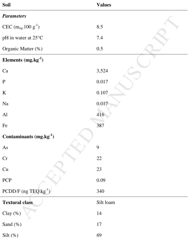
Table 2 presents some parameters of the sample X11Y12 of soil S3 and the initial concentrations of both organic and inorganic contaminants. This sample contained 0.5% of organic matter and its CEC was estimated at 8.5 meq.100g-1. The pH value of this soil was quite neutral (pH = 7.4). The elemental analysis of this sample revealed relatively low calcium, phosphorus, potassium and sodium contents with values reaching 3,524; 0.017; 0.107 and 0.017 mg.kg-1, respectively, and a concentration in iron and aluminum of 416 mg.kg-1 and 387 mg.kg-1, respectively. This entire soil sample was chosen because it contained a low concentration of organic contaminants. Indeed, it contained 9 mg As.kg-1, 22 mg Cr.kg-1, 23 mg Cu.kg-1, 0.09 mg PCP.kg-1 and 340 ng TEQ.kg-1 (PCDD/F). The distribution study of the particles' size by laser granulometry of the fraction less than 0.125 µm of the X11 Y12 sample, revealed that 14% of these particles were less than 2 µm, 69% were between 2 and 50 µm and 17% were between 50 and 2,000 µm. The texture of entire soil is silty loam (CEPP, 1987) .

3.2 Spatial distribution and descriptive statistics

An implementation map (Fig. 2) as well as a descriptive table (Table 3) of the exploratory statistics have been established for each contaminant (As, Cr, Cu, PCP and PCDD/F) present on the site by using MATLAB Software. A quick visualization of the data on the implantation maps established for the different contaminants gave a first idea of the spatial distribution of the contaminants. For the samples B1, B2 and B3 (background noise), the results highlighted a contamination inferior than cut-off 2 for the five contaminants, supporting the choice of their location. High contamination of PCP and of PCDD/F, exceeding cut-off 3 could be detected in

M

AN

US

CR

IP

T

AC

CE

PT

ED

the northwestern part of the site as well as a slight contamination of As (> cut-off 2). Moreover, it appeared that the concentration of both organic and inorganic contaminants were more important in the first 15 centimeters in almost location (except X8Y0P1 for PCP) and had tendency of decreasing with the depth, which is in accordance with the results obtained by Lespagnol (2003).

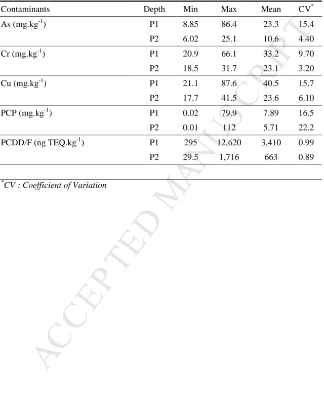
Following As contamination, the results indicated that As contents varied from 8.85 to 86.4 mg.kg-1 for P1 and from 6.02 to 25.1 mg.kg-1 for P2. Average contents and standard deviation were estimated at 23.3 ± 15.4 mg.kg-1 for P1 and 10.6 ± 4.4 mg.kg-1 for P2. The implementation map indicated an excess of the cut-off 3 (50 mg.kg-1) for a single sample (X10Y4P1) and an excess of the cut-off 2 (30 mg/kg) for only 4 samples among the 54 samples collected (X9Y1P1, X0Y3P1, X4Y8P1 and X11Y11P1). Moreover, no contamination was observed for the depth 2 (15-30 cm), indicating that the mobility of As was restricted to the first 15 cm, which is in accordance with the results obtained by Lespagnol (2003). The established implementation maps for the Cr and the Cu revealed a contamination superior to the cut-offs 2 (250 mg.kg-1 for Cr and 100 mg.kg-1 for Cu) for both depths P1 and P2, with average contents of 33.2 mg Cr.kg-1 for P1 and 23.1 mg Cr.kg-1 for P2. For Cu, average contents were estimated at 40.5 mg.kg-1 and23.6 mg.kg-1 for P1 and P2, respectively, indicating that the contamination was more important at the surface (0-15 cm).

The PCP implantation map showed an excess of the cut-off 4 (74 mg.kg-1) of PCP for samples X4Y2P1 and X8Y0P2 and an excess of the cut-off 3 (5 mg.kg-1) for 6 samples derived from P1 and for 1 sample derived from P2, with average contents estimated at 7.89 mg.kg-1 for P1 and 5.71 mg.kg-1 for P2. According to the PCDD/F implementation map, an important contamination of the northwestern part of the site was observed. Indeed, 5 samples found in P1 revealed

M

AN

US

CR

IP

T

AC

CE

PT

ED

contents above the cut-off 4 (5,000 ng TEQ.kg-1) for P1 and several samples in P1 and P2 revealed levels above cut-off 3 (750 ng TEQ.kg-1). According to the results presented in Table 3, PCDD/F contents varied from 295 to 12,620 ng TEQ.kg-1 for P1 and from 29.5 to 1,716 ng TEQ.kg-1 for P2, indicating a huge heterogeneity of PCDD/F contamination on the considered site.

Considering that the contamination of As, of Cr and of Cu come from the CCA-treated wood and that the PCP and PCDD/F contamination come from the PCP-treated wood, correlation studies have been performed on the following variables: (As-Cr), (As-Cu), (Cr-Cu), (PCP- PCDD/F) for both depth P1 and P2. The scatterplots between the variables (As, Cr and Cu), illustrated in Fig. 3, showed a satisfactory correlation between (As-Cr), (As-Cu) and (Cr-Cu) in P1 with respective correlation coefficients of 0.885 - 0.889 and 0.897. These results also highlighted a slight decrease in the correlations existing between these contaminants with depth. Considering contamination coming from PCP-treated wood, the scatterplots obtained between PCP and PCDD/F variables showed a good correlation level for P1 (Fig. 3). This correlation level decreases by 50.9% in P2. This decrease of correlation between the contaminants with the observed depth in both clouds of points can be explained by the fact that the contaminants do not migrate in the same way in soils. In fact, several studies have demonstrated that the As, Cr, Cu and PCDD/F are distributed and immobilized during the first 30 cm, unlike PCP can migrate up to 60 cm (Khodadoust et al., 2005; Lespagnol, 2003; Subramanian, 2007). Besides, these studies have shown that these organic and inorganic contaminants are significantly higher near the source of pollution and tend to decrease rapidly with the depth.

M

AN

US

CR

IP

T

AC

CE

PT

ED

Based on these results, interpolations were computed for As, PCP and PCDD/F as the contamination of the site by Cr and Cu was very low (cut-off 2) compared to As (cut-off 3), PCP (cut-offs 3 and 4) and PCDD/F (cut-offs 3 and 4).

3.3 Geostatistical analysis

The parameters of the semivariograms and variogram models chosen for As, PCP and PCDD/F that were used for OK and SGS methods, are presented in Table 4 (a) and (b), respectively. Unlike for OK method, a Gaussian transformation of the data was performed for SGS method before the semi-variogram calculation and back-transformed to original space after simulation in Gaussian space. The absence of contamination by As in P2 and by Cr and Cu in P1and P2 is noticed in Table 4 (a) and (b). This absence is due to the low contents of these contaminants (contents < cut-off 3). All experimental variograms for either OK or SGS were adjusted to a spherical model for each of the contaminants in P1 and P2. Besides, in all the variograms of contaminants, a nugget effect was observed (a discontinuity at the origin of the variograms representing noise level or short spatial structures not sampled). This nugget effect is probably due to the fact that soil pollution generally develops in a complex and heterogeneous environment (Jeannée, 2001). The ratio (Nugget / Sill) is considered as a criterion for classifying the spatial dependence of contaminant content (Chang et al., 1998; Chien et al., 1997). This ratio ranged from 9 to 56% for OK (Table 4 (a)) and from 30% to 39% for SGS (Table 4 (b)). Contaminant contents for As - P1, PCP - P1 and PCDD/F - P1 from OK had a strong spatial dependence since the ratio (Nugget / Sill) is less than 25%. However, for PCP - P2 and PCDD/F - P2, this ratio was moderate with values between 25 and 75%. For SGS, this ratio ranged from 30 to 39%, indicating that the spatial dependence of the contents was moderate for each contaminant in both P1 and P2.

M

AN

US

CR

IP

T

AC

CE

PT

ED

In contaminated site characterization, geostatistical methods have been used to estimate the volumes of soils whose concentration exceeds a regulatory criterion, to calculate the probabilities of exceeding regulatory criteria and to evaluate the uncertainty of these estimations (Boudreault

et al., 2016).

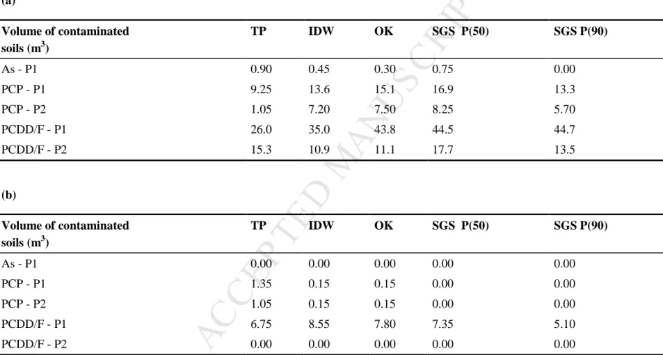
In the present study, soil volumes contaminated by As, PCP and PCDD/F were estimated from three interpolation methods (TP, IDW, OK) versus SGS, for both P1 and P2, except for As - P2 because the contamination was proven to be non-existent. Actually, these interpolation methods were chosen since they are the most commonly used to estimate volumes of contaminated sites. Table 5 presents the volume of soils contaminated by As, PCP or PCDD/F calculated using these methods. Table 5 (a) shows the volume of soil contaminated with values between cut-off 3 and cut-off 4 whereas Table 5 (b) shows the volume of soil contaminated with values that are above cut-off 4. According to the guide we referred to, the management of these soils is different depending on the cut-off value considered. In fact, beyond the cut-off 4 defined in Table 1, soils must be managed as dangerous residual materials, or treated to reach one of the cut-offs 1, 2, 3 or 4. Nowadays, the only available option for the remediation of these sites dealing with mixed contamination includes thermal treatment to destroy organic contaminants (PCP, PCDD/F) followed by immobilization of inorganic contaminants (As, Cr, Cu) through stabilization/solidification or landfilling (Kumpiene et al., 2016, Metahni et al., 2017). The cost of managing volumes of contaminated soils exceeding the cut-offs 4 is very expensive compared to volumes of contaminated soils between the cutt-offs 3 and cut-offs 4. A good estimation of volumes of contaminated soils allows for deciding about areas to be excavated and/or treated. Consequently, the cost of treatment can be accurately estimated. Results presented in Table 5 showed that PCDD/F contamination in P1 is the most problematic in this case, with volumes

M

AN

US

CR

IP

T

AC

CE

PT

ED

ranging from 26 to 45 m3 for P1 when the cut-off is between 750 and 5,000 ng TEQ.kg-1 and from 6.65 to 8.55 m3 when the cut-off is greater than 5,000 ng TEQ.kg-1. These results also showed that the contamination tends to decrease with depth (volume of contaminated soils less important in P2 compared with P1). These results can be explained by the fate and transport of metals, PCP and PCDD/F when they are released to the environment, due to the different physical and chemical properties of these contaminants and their different degree of affinity for the intrinsic components of soils (Guemiza et al., 2017). Besides, the results showed similarities in the estimations of the amounts of contaminated soils obtained by OK and SGS for PCP and PCDD/F unlike the other interpolation methods. Indeed, OK is considered as a better estimator of the mean and is more advanced than other interpolation methods such as TP and IDW (Cui et

al., 2016), since kriging considers two sets of distances (the distance between two sample

locations and the distance between a location of interest and a sample location) (Ha et al., 2014, Hou et al., 2017). However, the estimations of volume of soils contaminated by As was proven to be different depending on the method used, varying from 0.30 to 0.90 m3 and this can be explained by a very strong variation in the contents of As, which is often smoothed by the OK method. This smoothing effect can be observed when comparing kriged map of As, PCP and PCDD/F with the simulated map in the depth P1 (Supplementary Fig. 1). Both interpolations methods TP and IDW gave different volume estimations than OK and SGS considering the limitations of each of these methods. Even if TP estimation method is considered as a very simple method since it takes into account the content of a sample as block content, it neglects an extremely important factor which is the support effect (Armstrong et al., 1997), which often leads to an underestimation or an overestimation of contaminated soil volumes. Considering the IDW method, it is one of the most used spatial interpolation methods due to its fast

M

AN

US

CR

IP

T

AC

CE

PT

ED

implementation, ease of use and straightforward interpretation (Bhunia et al., 2016). However, it is indifferent to the geometric configuration of the observation sites. Indeed, only the distance with respect to the point counts, which results in the overweighting of the data groups. Unlike the OK in the case of regionalized variables, this method allows the estimation of the variable studied at each point of the considered field from the experimental data, the variogram and provides a variance of the error of the associated estimate (Juang et al., 2004). If the baseline conditions of the random function are met, OK will always be a better estimator of the mean than the other methods previously described (Cui et al., 2016). Numerous studies have demonstrated the performance of kriging compared to IDW for mapping soil properties (Kravchenko and Bullock, 1999, Mueller et al., 2004). However, OK tends to smooth out local details of the spatial variation in contaminant concentration. This is the reason why these linear interpolation methods do not allow the calculation of probabilities of exceedance of contamination thresholds. Indeed, smooth interpolated maps of soil contamination might cause unnecessary remediation of clean areas or overlook health hazards in contaminated areas. This smoothing effect has been clearly demonstrated in the study of Zawadzki et al. (2008), which was conducted for reassessment of soil contamination with lead. According to their results, the lead content maps showed that kriged values were smoothed from the range of 1-286 mg.kg-1 to the range of 1-90 mg.kg-1, unlike simulated map who reproduced better the range of variability of lead contents in soils. In this case, non-linear methods such as indicator kriging or simulations can and should be used. Indeed, the interpolators are estimators of the mean. Therefore, they are not suitable for reproducing the upper and lower quantiles. While a simulation is a possible realization of the contaminant contents on the studied field, which reproduces the spatial variability of the studied phenomenon while respecting the histogram and the variogram of the

M

AN

US

CR

IP

T

AC

CE

PT

ED

measured contents. Applying a concentration threshold to a conditional simulation provides an unbiased estimator of contaminant levels above the defined threshold (Boudreault et al., 2016). This is why SGS is the most appropriate method to use in order to estimate the volumes of contaminated soil.

3.4 Risk assessment

The SGS interest lies in the fact of calculating a large number of scenarios, allowing a reasoning in probabilities. In each estimated mesh, we have a histogram of the possible values (equi-probable), whose average converges towards the kriging. By calculating point by point, the proportion of realization exceeds a certain cut-off. As a result, it produces a map estimating the probability of exceeding the risk cut-offs, which will be used for risk assessment and decision-making. Actually, Fig. 4 illustrates the post-treatment of surfaces whose PCDD/F concentrations exceed the cut-off 3 (750 ng TEQ/kg) and the cut-off 4 (5,000 ng TEQ/kg) for both P1 and P2. Fig. 4a proved that in the case where the PCDD/F concentrations exceed cut-off 3, the P50 shows reasonable surfaces to be treated were estimated at 330 m2 for P1 and 116 m2 for P2, with a 90% confidence interval between 310 and 346 m2 for PCDD/F-P1 and between 86 and 148 m2 for PCDD/F-P2. However, when PCDD/F concentrations exceed cut-off 4, it is expected to treat an area of approximately 49 m2 only for P1 with a 90% confidence interval between 30 and 73 m2 (Fig. 4b). This information is critical for decision-makers to determine which contaminated areas can be disposed directly in a sanitary landfill (areas between cut-off 3 and cut-off 4), and which areas require treatment by thermal desorption to destroy organic contaminants (PCP, PCDD/F) followed by solidification/stabilization of inorganic contaminants (As, Cr, Cu – areas exceeding cut-off 4) or landfilling (areas exceed cut-off 3).

M

AN

US

CR

IP

T

AC

CE

PT

ED

Once defined, these risk curves will be used to assess the financial risks associated with the rehabilitation of this site. These risks will be estimated by applying a cost function to geostatistical estimates of soil volumes to be treated and their accuracy. Then, a sorting scheme has to be defined considering that only the blocks showing concentrations of contaminants above the cut-offs will be sent to a treatment channel or to be disposed in landfills.

4

C

Nowadays, soil characterization is a major challenge for the rehabilitation of contaminated sites. In fact, an erroneous interpretation of the state of contamination of a site may have serious consequences such as health issues and/or financial losses. This study aims to show the relevance of the geostatistics application in the case of industrial soils contaminated by both organic (PCP and PCDD/F) and inorganic (As, Cr, Cu) contaminants.

The exploratory analysis of the experimental data using the geostatistical tool revealed a perfect correlation between (As-Cr), (As-Cu) and (Cr-Cu) in P1, which slightly decreased with depth and a good level of correlation between PCP and PCDD/F for P1, which decreased by 50.9% in P2. Experimental variograms showed a nugget effect related to the heterogeneity of contaminant levels in the studied site.

In this project, a comparative study of two conventional interpolation methods versus geostatistical OK and SGS methods was conducted in order to evaluate the performance of each of these methods in estimating volumes of contaminated soils. The TP and IDW methods are interpolation methods that predict the value of a point only on the basis of the values of the points in the neighborhood and do not take into account the spatial structure of the data. For this reason, OK always remains a better estimator of the mean comparing to both other methods of

M

AN

US

CR

IP

T

AC

CE

PT

ED

interpolation if the variable under study shows a spatial correlation. However, OK provides a smoothed image of reality while also not allowing the calculation of probabilities of exceeding regulatory cut-offs of contamination. SGS had been proved to be the most suitable method for estimating volumes of soils contaminated with As, PCP and PCDD/F, and to quantify the uncertainty of estimates associated with the volumes calculations. These estimates will be relevant to select the most appropriate treatment in our case and to accurately assess the financial risk of this rehabilitation project.

Sample density by SGS depends on the sampling area and allocated budget. In the case of mixed contamination by organic (PCP, PCDD/F) and inorganic (As, Cr, Cu) compounds, the choice of the number of samples and the geostatistical approach is often guided by the budget allocated to the analysis of PCDD/F. The industrials are often forced to adopt other approaches than SGS like TP, to minimize the number of samples and to avoid the costly analyzes of organic contaminants. Supplemental research will be done to optimize the location and the number of sampling holes during a sampling campaign in order to reduce the cost of PCDD/F analysis and to establish the best strategy for the rehabilitation of these sites. It would also be interesting to combine GIS with multivariate data analysis in this case of contamination, because GIS and PCA represent powerful tools in decision-making on future investigations, risk assessments and remediation of contaminated sites.

Acknowledgments

This work was supported by the Natural Sciences and Engineering Research Council of Canada and IREQ under grant RDC 463019-14 and the Canada Research Chairs Program.

M

AN

US

CR

IP

T

AC

CE

PT

ED

R

APHA, 1999 Standards methods for examination of water and wastewaters. 20th Edition. American Public Health Association. Washington, DC, USA, 541 p.

Armstrong, M., Garignan, J., 1997. Géostatistique linéaire: Application au domaine minier. Sciences de la terre et de l'environnement. École des mines de Paris, Les Presses, Paris, France,112 p.

Arnaud, M., Emery, X., 2000. Estimation et interpolation spatiale : Méthodes déterministes et méthodes géostatistiques. Hermes science publications, Paris, France, 217 p.

Atteia, O., Dubois, J.P., Webster, R., 1994. Geostatistical analysis of soil contamination in the Swiss Jura. Environmental Pollution 86(3), 315-327, https://doi.org/10.1016/0269-7491(94)90172-4.

Bartier, P.M., Keller, C.P., 1996. Multivariate interpolation to incorporate thematic surface data using inverse distance weighting (IDW). Computers & Geosciences 22(7), 795-799, https://doi.org/10.1016/0098-3004(96)00021-0.

Bhunia, G.S., Shit, P.K., Maiti, R., 2016. Comparison of GIS-based interpolation methods for spatial distribution of soil organic carbon (SOC). Journal of the Saudi Society of

Agricultural Sciences 17(2), 114-126, https://doi.org/10.1016/j.jssas.2016.02.001.

Bobbia, M., Pernelet, V., Roth, C., 2001. L'intégration des informations indirectes à la cartographie géostatistique des polluants. Pollution atmosphérique N° 170, 251-262, https://doi.org/10.4267/pollution-atmospherique.2757.

Boudreault, J.P., Dubé, J.S., Marcotte, D., 2016. Quantification and minimization of uncertainty by geostatistical simulations during the characterization of contaminated sites: 3-D approach to a multi-element contamination. Geoderma 264, 214-226, https://doi.org/10.1016/j.geoderma.2015.10.019.

Burgos, P., Madejón, E., Pérez-de-Mora, A., Cabrera, F., 2006. Spatial variability of the chemical characteristics of a trace-element-contaminated soil before and after

remediation. Geoderma 130(1), 157-175,

https://doi.org/10.1016/j.geoderma.2005.01.016.

CCME, 1993. Guide pour l'échantillonnage, l'analyse des échantillons et la gestion des données des lieux contaminés. Volume I : Rapport principal. Rapport CCME EPC NCS62F, Programme national des lieux contaminés, Le conseil canadien des ministres de l'environnement, Ottawa, ON, Canada, 90 p.

Chang, Y.H., Scrimshaw, M.D., Emmerson, R.H.C., Lester, J.N., 1998. Geostatistical analysis of sampling uncertainty at the Tollesbury managed retreat site in Blackwater Estuary, Essex, UK: kriging and cokriging approach to minimise sampling density. Science of the Total Environment 221, 43-57, https://www.sciencebase.gov/catalog/item/5053d8d2e4b097 cd4fcf35ba.

Chien, Y.L., Lee, D.Y., Guo, H.Y., Houng, K.H., 1997. Geostatistical analysisof soil properties of mid-west Taiwan soils. Soil Science 162, 291-297, http://dx.doi.org/10.1097/00010694-199704000-00007.

M

AN

US

CR

IP

T

AC

CE

PT

ED

CEAEQ, 2003. Détermination de la matière organique par incinération : Méthode de perte de feu (PAF), MA. 1010 – PAF 1.0. Centre d'Expertise en Analyse Environnementale du Québec, Québec, QC, Canada, 9 p.

CEAEQ, 2011. Détermination des dibenzo-para-dioxines polychlorés et dibenzofuranes polychlorés : Dosage par chromatographie en phase gazeuse couplée à un spectromètre de masse, MA. 400 – D.F. 1.1. Centre d'Expertise en Analyse Environnementale du Québec, Québec, QC, Canada, 33 p.

CEAEQ, 2013. Détermination des composés phénoliques : dosage par chromatographie en phase gazeuse couplée à un spectromètre de masse après dérivation avec l'anhydride acétique, MA. 400 – Phé 1.0, Rév. 3. Centre d'Expertise en Analyse Environnementale du Québec, Québec, QC, Canada, 20 p.

CEPP, 1987. Le système Canadien de classification des Sols (3ième Édition). Publication 1646, Comité d'Experts sur la Prospection Pédologique, Agriculture Canada, Ottawa, ON, Canada, 187 p.

Coudert, L., Blais, J.F., Mercier, G., Cooper, P., Morris, P., Gastonguay, L., Janin, A., Zaviska, F., 2013. Optimization of copper removal from ACQ-, CA-, and MCQ-treated wood using an experimental design methodology. Journal of Environmental Engineering -

ASCE 139(4), 576-587, https://doi.org/10.1533/9780857096906.4.526.

Cui, Y.Q., Yoneda, M., Shimada, Y., Matsui, Y., 2016. Cost-effective strategy for the investigation and remediation of polluted soil using geostatistics and a genetic algorithm approach. Journal of Environmental Protection 7, 99-115, https://doi.org/10.4236/jep.2016.71010.

Delbari, M., Afrasiab, P., Loiskandl, W., 2009. Using sequential Gaussian simulation to assess the field-scale spatial uncertainty of soil water content. CATENA 79(2), 163-169, https://doi.org/10.1016/j.catena.2009.08.001.

Demougeot-Renard, H., De Fouquet, C., 2004. Geostatistical approach for assessing soil volumes requiring remediation: validation using lead-polluted soils underlying a former smelting works. Environmental Science and Technology 38(19), 5120-5126, https://doi.org/ 10.1021/es0351084.

Fabijańczyk, P., Zawadzki, J., Magiera, T., 2017. Magnetometric assessment of soil contamination in problematic area using empirical Bayesian and indicator kriging: A case study in Upper Silesia, Poland. Geoderma 308, 69-77, https://doi.org/10.1016/j.geoderma.2017.08.029.

Facchinelli, A., Sacchi, E., Mallen, L., 2001. Multivariate statistical and GIS-based approach to identify heavy metal sources in soils. Environmental Pollution 114(3), 313-324, https://doi.org/10.1016/S0269-7491(00)00243-8.

GeoSIPOL, 2005. Les pratiques de la géostatistique dans le domaine des sites et sols pollués. Géostatistique appliquée aux sites et sols pollués. Manuel méthodologique et exemple d'applications, GeoSIPOL, France, 139 p.

Goovaerts, P., 1999. Geostatistics in soil science: state-of-the-art and perspectives. Geoderma 89(1), 1-45, https://doi.org/10.1016/S0016-7061(98)00078-0.

M

AN

US

CR

IP

T

AC

CE

PT

ED

Guemiza, K., Coudert, L., Metahni, S., Mercier, G., Besner, S., Blais, J.F., 2017. Treatment technologies used for the removal of As, Cr, Cu, PCP and/or PCDD/F from contaminated soil: A review. Journal of Hazardous Materials 333, 194-214, https://doi.org/10.1016/j.jhazmat.2017.03.021.

Ha, H., Olson, J.R., Bian, L., Rogerson, P.A., 2014. Analysis of heavy metal sources in soil using kriging interpolation on principal components. Environmental Science and

Technology 48(9), 4999-5007, https://doi.org/10.1021/es405083f.

Henriksson, S., Hagberg, J., Bäckström, M., Persson, I., Lindström, G., 2013. Assessment of PCDD/Fs levels in soil at a contaminated sawmill site in Sweden – A GIS and PCA approach to interpret the contamination pattern and distribution. Environmental Pollution 180, 19-26, https://doi.org/10.1016/j.envpol.2013.05.002.

Hou, D., O'Connor, D., Nathanail, P., Tian, L., Ma, Y., 2017. Integrated GIS and multivariate statistical analysis for regional scale assessment of heavy metal soil contamination: A critical review. Environmental Pollution 231, 1188-1200, https://doi.org/10.1016/j.envpol.2017.07.021.

Jeannée, N., 2001. Caratérisation géostatistique de pollutions industrielles de sols: Cas des hydrocarbures aromatiques polycycliques sur l'anciens sites de cokeries. PhD report, École des mines de Paris, Paris, France, 201 p.

Jin, Y., O'Connor, D., Ok, Y.S., Tsang, D.C.W., Liu, A., Hou, D., 2019. Assessment of sources of heavy metals in soil and dust at children's playgrounds in Beijing using GIS and multivariate statistical analysis. Environment International 124, 320-328, https://doi.org/10.1016/j.envint.2019.01.024.

Juang, K.W., Chen, Y.S., Lee, D.Y., 2004. Using sequential indicator simulation to assess the uncertainty of delineating heavy-metal contaminated soils. Environmental Pollution 127(2), 229-238, https://doi.org/10.1016/j.envpol.2003.07.001.

Khodadoust, A.P., Reddy, K.R., Maturi, K., 2005. Effect of different extraction agents on metal and organic contaminant removal from a field soil. Journal of Hazardous Materials 117(1), 5-24, https://doi.org/10.1016/j.jhazmat.2004.05.021.

Kravchenko, A.N., 2003. Influence of spatial structure on accuracy of interpolation methods. Soil Science Society American Journal 67,1564-1571, https://doi.org/ 10.2136/sssaj2003.1564.

Kravchenko, A., Bullock, D.G., 1999. A comparative study of interpolation methods for mapping soil properties. Agronomy Journal 91, 393-400, https://doi.org/10.2134/agronj1999.00021962009100030007x.

Kumpiene, J., Nordmark, D., Hamberg, R., Carabante, I., Simanavičienė, R., Aksamitauskas, V.Č. 2016. Leaching of arsenic, copper and chromium from thermally treated soil.

Journal of Environmental Management 183, 460-466,

https://doi.org/10.1016/j.jenvman.2016.08.080.

Lark, R.M., Ferguson, R.B., 2004. Mapping risk of soil nutrient deficiency or excess by disjunctive and indicator kriging. Geoderma 118(1), 39-53, https://doi.org/10.1016/S0016-7061(03)00168-X.

M

AN

US

CR

IP

T

AC

CE

PT

ED

Lespagnol, G., 2003. Lixiviation du chrome, du cuivre et de l’arsenic (CCA) à partir de sols contaminés sur des sites de traitement du bois. Ph.D. Thesis, École Nationale Supérieure des Mines de Saint-Étienne et de l’Université Jean Monnet, France, 212 p.

Lin, W.C., Lin, Y.P., Wang, Y.C., 2016. A decision-making approach for delineating sites which are potentially contaminated by heavy metals via joint simulation. Environmental

Pollution 211(Supplement C), 98-110, https://doi.org/10.1016/j.envpol.2015.12.030.

Lin, Y.P., Chang, T.K., Teng, T.P., 2001. Characterization of soil lead by comparing sequential gaussian simulation, simulated annealing simulation and kriging methods. Environmental

Geology 41, 189-199, https://doi.org/10.1016/j.envpol.2015.12.030.

Liu, X., Zhao, K., Xu, J., Zhang, M., Si, B., Wang, F., 2008. Spatial variability of soil organic matter and nutrients in paddy fields at various scales in southeast China. Environmental

Geology 53, 1139-1147, https://doi.org/ 10.1007/s00254-007-0910-8.

McGrath, D., Zhang, C., Carton, O.T., 2004. Geostatistical analyses and hazard assessment on soil lead in Silvermines area, Ireland. Environmental Pollution 127(2), 239-248, https://doi.org/10.1016/j.envpol.2003.07.002.

Metahni, S., Coudert, L., Chartier, M., Blais, J.F., Mercier, G., Besner, S., 2017. Pilot-scale decontamination of soil polluted with As, Cr, Cu, PCP, and PCDDF by attrition and alkaline leaching. Journal of Environmental Engineering ASCE 143(9), 04017055, https://doi.org/10.1061/(ASCE)EE.1943-7870.0001255.

Metson, A.J., 1956. Methods of chemical analysis for soil survey samples. NZ Soil Bur Bull n°12.

Mu, L., 2009. Thiessen Polygon. International Encyclopedia of Human Geography, Kitchin R & Thrift N (Édit.) Elsevier, Oxford. p 231-236. https://doi.org/10.1016/B978-008044910-4.00545-9.

Mueller, T.G., Pusuluri, N.B., Mathias, K.K., Cornelius, P.L., Barnhisel, R.I., Shearer, S.A., 2004. Map quality for ordinary kriging and inverse distance weighted interpolation. Soil

Science Society of America Journal 68, 2042-2047,

https://doi.org/10.2136/sssaj2004.2042.

Ordoñez, J.A., Bandyopadhyay, D., Lachos, V.H., Cabral, C.R.B., 2018. Geostatistical estimation and prediction for censored responses. Spatial Statistics 23, 109-123, https://doi.org/10.1016/j.spasta.2017.12.001 .

PCA, 2009. Guidelines for the use, handling and disposal of treated wood. Parks Canada Agency, Ottawa, ON, Canada, 25 p.

Saito, H., Goovaerts, P., 2000. Geostatistical Interpolation of Positively Skewed and Censored Data in a Dioxin-Contaminated Site. Environmental Science Technology 34(19), 4228– 4235, https://doi.org/10.1021/es991450y

Shen, F., Liao, R., Ali, A., Mahar, A., Guo, D., Li, R., Xining, S., Awasthi, M.K., Wang, Q., Zhang, Z., 2017. Spatial distribution and risk assessment of heavy metals in soil near a Pb/Zn smelter in Feng County, China. Ecotoxicology and Environmental Safety 139, 254-262, https://doi.org/10.1016/j.ecoenv.2017.01.044.

M

AN

US

CR

IP

T

AC

CE

PT

ED

Subramanian, B., 2007. Exploring Neoteric Solvent Extractants: Applications in the Removal of Sorbates From Solid Surfaces and Regeneration of Automotive Catalytic Converters. Division of research and advanced studies, University of Cincinnati, Ohio, USA, 82 p. Vauclin, M., Vieira, S.R., Bernard, R., Hatfield, J.L., 1982. Spatial variability of surface

temperature along two transects of a bare soi. Water Resources Research 18(6), 1677-1686, https://doi.org/10.1029/WR018i006p01677.

Xie, Y., Chen, T.B., Lei, M., Yang, J., Guo, Q.J., Song, B., Zhou, X.Y., 2011. Spatial distribution of soil heavy metal pollution estimated by different interpolation methods: Accuracy and uncertainty analysis. Chemosphere 82(3), 468-476, https://doi.org/10.1016/j.chemosphere.2010.09.053.

Zawadzki, J., Fabijańczyk, P., 2008. The geostatistical reassessment of soil contamination with lead in metropolitan Warsaw and its vicinity. International Journal of Environment and

Pollution 35(1), 1-12, https://doi.org/10.1504/IJEP.2008.021127.

Zawadzki, J., Szuszkiewicz, M., Fabijańczyk, P., Magiera, T., 2016. Geostatistical discrimination between different sources of soil pollutants using a magneto-geochemical data set. Chemosphere 164, 668-676, https://doi.org/10.1016/j.chemosphere.2016.08.145.

M

AN

US

CR

IP

T

AC

CE

PT

ED

FIGURE CAPTIONS LIST

Fig. 1. Location of the 27 exploration holes at the treated wood storage site

Fig. 2. Implantation maps of As (a.), Cr (b.), Cu (c.), PCP (d.) and PCDD/F (e.) samples in P1 (0 to 0.15 m – value in blue) and in P2 (0.15 to 0.30 m – value in red) (As, Cr, Cu and PCP concentrations are expressed in mg.kg-1 and PCDD/F content expressed in ng TEQ.kg-1)

Fig. 3. Correlation between (As-Cr), (As-Cu) and (Cr-Cu) at P1 from 0 to 0.15 m (a.) and P2 from 0.15 to 0.3 m (b.), Correlation between (PCP-PCDD/F) (c.) Fig. 4. Post-treatment of areas with PCDD/F concentrations exceeding

750 ngTEQ.kg-1 at P1 (a.) and P2 (b.) or 5,000 ngTEQ.kg-1 at P1 (c.) and P2 (d.)

SUPPLEMENTARY FIGURE CAPTIONS LIST

Fig. 1. Maps of As, PCP and PCDDF concentrations in soils obtained by OK and SGS methods at P1 from 0 to 0.15 m: (OK) As P1 (a.), (SGS) As P1 (b.), (OK) PCP P1 (c.), (SGS) PCP P1 (d.), (OK) PCDDF P1 (e.), (SGS) PCDDF P1 (f.)

M

AN

US

CR

IP

T

AC

CE

PT

ED

Table 1 Cut-offs defined for the estimation of soil contamination in rehabilitation scenario Contaminants As (mg.kg-1) Cr (mg.kg-1) Cu (mg.kg-1) PCP (mg.kg-1) PCDD/F (ng TEQ.kg-1) Cut-off 1 6 85 40 0.1 - Cut-off 2 30 250 100 0.5 15 Cut-off 3 50 800 500 5 750 Cut-off 4 250 4,000 2,500 74 5,000

M

AN

US

CR

IP

T

AC

CE

PT

ED

Table 2 Soil parameters measured in the sample X11 Y12 P1 of soil S3

Soil Values Parameters CEC (meq.100 g-1) 8.5 pH in water at 25°C 7.4 Organic Matter (%) 0.5 Elements (mg.kg-1) Ca 3,524 P 0.017 K 0.107 Na 0.017 Al 416 Fe 387 Contaminants (mg.kg-1) As 9 Cr 22 Cu 23 PCP 0.09 PCDD/F (ng TEQ.kg-1) 340

Textural class Silt loam

Clay (%) 14

Sand (%) 17

Silt (%) 69

M

AN

US

CR

IP

T

AC

CE

PT

ED

Table 3 Descriptive statistics of investigated data of As, Cr, Cu PCP and PCDD/F contents measured in contaminated soils

Contaminants Depth Min Max Mean CV*

As (mg.kg-1) P1 8.85 86.4 23.3 15.4 P2 6.02 25.1 10.6 4.40 Cr (mg.kg-1) P1 20.9 66.1 33.2 9.70 P2 18.5 31.7 23.1 3.20 Cu (mg.kg-1) P1 21.1 87.6 40.5 15.7 P2 17.7 41.5 23.6 6.10 PCP (mg.kg-1) P1 0.02 79.9 7.89 16.5 P2 0.01 112 5.71 22.2 PCDD/F (ng TEQ.kg-1) P1 295 12,620 3,410 0.99 P2 29.5 1,716 663 0.89 * CV : Coefficient of Variation