This is an author-deposited version published in: http://oatao.univ-toulouse.fr/ Eprints ID: 5304
To cite this version:
Masmoudi, Malek and Haït, Alain Fuzzy uncertainty
modelling for project planning; application to helicopter maintenance.
(2012) International Journal of Production Research, vol. 50 (n° 13). pp.
3594-3611. ISSN 0020-7543
O
pen
A
rchive
T
oulouse
A
rchive
O
uverte (
OATAO
)
OATAO is an open access repository that collects the work of Toulouse researchers and makes it freely available over the web where possible.
Any correspondence concerning this service should be sent to the repository administrator: [email protected]
Fuzzy uncertainty modelling for project planning;
application to helicopter maintenance
Malek Masmoudi and Alain Ha¨ıt
Universit´e de Toulouse, Institut Sup´erieur de l’A´eronautique et de l’Espace 10 av. Edouard Belin 31055 Toulouse, France
Maintenance is an activity of growing interest specially for critical systems. Particularly, aircraft maintenance costs are becoming an important issue in the aeronautical industry. Managing an aircraft maintenance center is a complex activity. One of the difficulties comes from the numerous uncertainties that affect the activity and disturb the plans at short and medium term. Based on a helicopter maintenance planning and scheduling problem, we study in this paper the integration of uncertainties into tactical and operational multi-resource, multi-project planning (respectively Rough Cut Capacity Planning and Resource Constraint Project Scheduling Problem). Our main contributions are in modelling the periodic workload on tactical level considering uncertain-ties in macro-tasks work contents, and modelling the continuous workload on operational level considering uncertainties in tasks durations. We model uncer-tainties by a fuzzy/possibilistic approach instead of a stochastic approach since very limited data are available. We refer to the problems as the Fuzzy Rough Cut Capacity Problem (FRCCP) and the Fuzzy Resource Constraint Project Scheduling Problem (RCPSP). We apply our models to helicopter maintenance activity within the frame of the Helimaintenance project, an industrial project approved by the French Aerospace Valley cluster which aims at building a center for civil helicopter maintenance.
Keywords: Fuzzy/possibistic, Planning, Scheduling, PERT/CPM, Helicopters, maintenance.
1. Introduction
Aircraft maintenance consists of carrying out all the actions necessary to guarantee the required level of reliability, safety and operational capacity of the aircraft. A main characteristic of aeronautics is that maintenance is highly regulated, due to the potential criticality of failures. From a product point of view, various documents define aircraft maintenance. Among them, the maintenance planning document (MPD), established by the manufacturer on the basis of reliability studies, gives the periodicity of inspection of
the equipments (calendar limits and/or number of flight hours and/or number of take-off-landing flight cycles). The MPD is periodically updated so the maintenance tasks may change all along the aircraft life cycle. From a process point of view, the Aircraft Maintenance Manual describes how to perform the maintenance actions. Regulation also constrains the process: ratio of permanent operators, number of hours per week, and skills.
On this basis, the owner of the aircraft establishes the maintenance program, that must be approved by the authorities. The list of tasks to be performed during a maintenance visit depends on the aircraft exploitation and equipment history, while considering the limits set in the MPD. It also depends on decisions of anticipating some tasks in order to balance the number of visits and their durations (i.e., to balance aircraft exploitation and maintenance cost). Finally, unexpected failures may force to anticipate a visit.
Aeronautical maintenance visits are numerous; some are carried out on-line, like simple checks before and after flight or small inspections, others are generally subcontracted and carried out off-line, at a maintenance center. It is the case for Heavy Maintenance Visits (HMV). These visits affect all the aspects (structure, avionics, mechanics) and can last up to several months. On PUMA helicopters for example, HMV is generally carried out every twelve years and costs about two millions Euro (one third of the aircraft price).
Maintenance planning aims at organizing the activity of a maintenance center. It deals with the tasks to realize for each aircraft, the workforce and equipment organization, spare parts logistics (purchasing and inventory management). The challenge is to provide a minimum aircraft down time to the customers, while maintaining good productivity and inventory costs. This study focuses on planning and scheduling. We consider that spare parts logistics is out of the scope, and treat this aspect by introducing procurement delays.
The Helimaintenance project focuses on civil helicopter maintenance. In addition to the above considerations, helicopters have some specificities; particular flight conditions (vibrations, way of landing) involve high frequency of inspection for some equipments, limited volume may constrain the realization of tasks (number of operators concurrently working). Moreover, addressing civil customers involves a great heterogeneity of heli-copters. Indeed, the mean number of helicopters by civil owner is between two and three, and the conditions of use can radically vary from one customer to another (sea, sand, mountain...). The customization can also lead to very different equipment configurations. Hence the application of global optimization approaches, as can be found in the military domain for important homogeneous fleets and one single customer (Hahn and Newman 2008, Sgaslink 1994), is not pertinent in this case.
Next section presents the planning and scheduling processes for a maintenance center and describes the uncertainties that affect them. Section 3 recalls the state of art for fuzzy set and possibilistic approach, and their use in planning and scheduling problems under uncertainty. Sections 4 and 5 deal with fuzzy modelling in tactical and operational levels of planning. Each section contains an illustration from a helicopter maintenance activity.
2. Problem statement
The Heavy Maintenance Visits contain planned maintenance tasks and also corrective maintenance tasks since several failures are discovered during the initial inspection. Precedence constraints exist between the tasks, due to technical or accessibility
consider-ations. Hence a HMV may be seen as a project involving various resources as operators, equipment, and spare parts. As already noted, minimizing the overall visit duration give a competitive advantage to the company. Consequently, the management of a maintenance center is viewed as multi-project management, where every project duration should be minimized while respecting capacity constraints. Dealing with uncertainties is a main issue of helicopter maintenance planning. In this section we describe the specificities of the problem.
2.1. Tactical and operational project planning
Hans et al. (2007) classify multi-project organizations according to their projects vari-ability and dependency. In addition, they propose a hierarchical framework for multi-project planning and control. In the hierarchical axis, the framework is divided into the three levels of Anthony’s classification (strategic, tactical and operational) and in the functional axis it is divided into technological planning, capacity planning, and material coordination. Inspired from manufacturing, this framework is suitable to our problem that gathers production and project features. Following this reference, our problem is considered with high variability (numerous uncertainties) and high dependency (shared resources and external influence on spare parts supply).
Gademann and Schutten (2005) show the difference between Rough Cut Capacity Plan-ning (RCCP, tactical) and Resource-Constrained Project Scheduling Problem (RCPSP, operational). At the tactical level of planning, orders are studied and then prices and delivery times are negotiated with customers. After a project has been accepted, the macro-tasks are well specified and integrated into the global tactical plan. At the oper-ational level, macro-tasks are detailed into elementary tasks and resources are assigned to different tasks according to their capabilities. During tactical and operational plan-ning levels, dealing with capacity management problem is an important issue. In RCCP, the planning horizon is divided into periods contrary to RCPSP where time horizon is continuous. In RCCP the workload is defined in terms of macro-tasks work contents per required resources (e.g. a total of 150 hours of work content for Avionicians) in contrast to RCPSP where the tasks duration and the number of operators assigned to the tasks are considered (e.g. the task must be performed by 2 avionicians during 8 hours).
2.2. Uncertainties in planning and scheduling
Dealing with high variability is an important issue. The hierarchical decomposition aims at generating stable plans, coordinating levels and dealing with the adequate horizon and data at each level. At the tactical level, we can identify three main sources of uncertainty: • Uncertainty in the release date: a customer enters into a contract for a HMV several months before the helicopter entry in maintenance. According to the exploitation, the real start date may vary in order to reach the limits set by the MPD. The release date is fixed only 6 weeks earlier.
• Uncertainty in the workload: the corrective maintenance part is significant in these projects. The nature of the corrective maintenance is only known after the first in-spection tasks of the project.
• Uncertainty in procurement delays: though spare parts for planned maintenance can be purchased on time, corrective maintenance induce additional orders. Whether these parts are available in the inventory or should be purchased, or even must be
manufac-tured, the procurement delays may change radically.
And at the operational level, we can identify three main sources of uncertainty:
• Absence of operators: the unexpected lack of resources causes the delay of several tasks and hence some tasks’ durations are increased.
• Tasks durations: differs according to skills level of assigned operator. It differs also from one helicopter to another according to the compactness, state, and mission use. Tasks starting dates are consequently uncertain.
• Maintenance program updates: manufacturers and authorities send regularly new doc-uments (Service Bulletin, Airworthiness Directives, etc...) to add, eliminate or modify some tasks from the maintenance program document.
According to our knowledge the problem of tactical planning under uncertainty for aero-nautical maintenance, and the problem of civil aeroaero-nautical maintenance scheduling have never been studied. To deal with uncertainties in this case, we propose a combined ap-proach. First, considering the non repetitive aspect of the problem (each helicopter has its own history, the customers are numerous and the conditions of use are highly different), and the difficulty to predict the exploitation or establish statistics on corrective tasks or tasks durations, we propose a fuzzy set modelling for macro-tasks work contents to cope with uncertainty in tactical level of planning. Then uncertainty affecting the operational level is managed by a fuzzy set modelling for tasks’ dates and durations.
3. Fuzzy/possibilistic approach for planning
To deal with uncertainty, both fuzzy and stochastic modelling are used in literature depending on the quantity and quality of available information. Fuzzy modelling is more appropriate while few and imprecise information is available (Chen 2000), which is the case in helicopter maintenance domain (Masmoudi and Ha¨ıt 2010). Using stochastic computation usually starts by taking strong hypothesis while choosing distributions. In fact, when the real distribution of the uncertainty looks different than all known probability densities (exponential, beta, normal and others), stochastic arithmetic like convolution product becomes hardly applicable. Hence, the real distribution is usually estimated and simplified to fit with a known distribution. The strength of fuzzy modelling consists of respecting exactly what experts know about the uncertainty and no more. To be honest, small hypothesis are taken too while choosing the entire profile specially straight lines instead of curves (see section 3.1). Nevertheless, fuzzy arithmetic are easy to manipulate whatever the complexity of the profile considered.
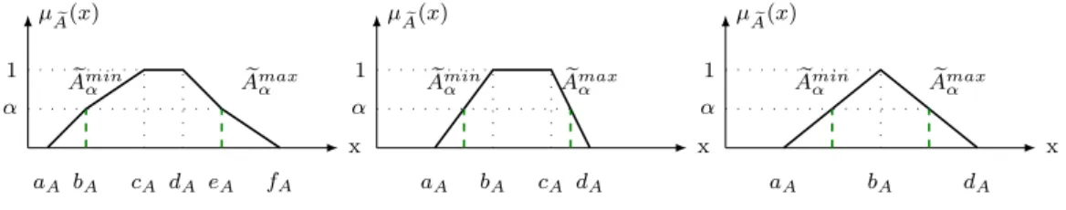
3.1. Fuzzy sets
Introduced by Zadeh (1965), the fuzzy set theory is well-suited to handle uncertainties in different domains specially in production management (Guiffrida and Nagi 1998). Many profiles are used in the literature to model fuzzy quantities (Figure 1). Particularly, the trapezoidal profile is well-supported by the possibility approach (see section 3.2).
Zadeh has defined a fuzzy set eA as a subset of a referential set X, whose boundaries are gradual rather than abrupt. Thus, the membership function µAeof a fuzzy set assigns to each element x ∈ X its degree of membership µAe(x) taking values in [0,1].
To generalize some operations from classical logic to fuzzy sets, Zadeh has given the possibility to represent a fuzzy profile by an infinite family of intervals called α-cuts.
Hence, the fuzzy profile eA can be defined as a set of intervals Aα= {x ∈ X/µAe(x) ≥ α}
with α ∈ [0, 1]. It became consequently easy to utilize classical interval arithmetic and adapt it to fuzzy profiles.
µ e A(x) 1 α x aA bA cA dA e Amin α Aemaxα µ e A(x) 1 α x aA bA cA dA eA fA e Amin α Aemaxα µ e A(x) 1 α x aA bA dA e Amin α Aemaxα
Figure 1. Some fuzzy profiles.
Dubois and Prade (1988b), and Chen and Hwang (1992) have defined mathematical operations that can be performed on trapezoidal fuzzy sets.
Let eA(aA, bA, cA, dA) and eB(aB, bB, cB, dB) be two independent trapezoidal fuzzy
num-bers, then:
e
A ⊕ eB = (aA+ aB, bA+ bB, cA+ cB, dA+ dB) (1)
e
A eB = (aA− dB, bA− cB, cA− bB, dA− aB) (2)
min( eA, eB) = (min(aA, aB), min(bA, bB), min(cA, cB), min(dA, dB)) (3)
max( eA, eB) = (max(aA, aB), max(bA, bB), max(cA, cB), max(dA, dB)) (4)
e A ∪ eB = max x∈X(µAe(x), µBe(x)) (5) e A ∩ eB = min x∈X(µAe(x), µBe(x)) (6) α eA = ( (αaA, αbA, αcA, αdA) if α > 0 (αdA, αcA, αbA, αaA) if α < 0 (7)
Other operations like multiplication and division have also been studied. For more details regarding fuzzy arithmetic we refer readers to Dubois and Prade (1988b).
3.2. Possibility theory
The possibility theory is based on fuzzy subsets. It was introduced by Zadeh (1978) to provide a mean to take into account the uncertainties while event occurs. Since we have chosen a fuzzy model, we will use the possibility theory to transpose uncertainty in data into uncertainty in workload.
The possibility theory introduces both a possibility measure (denoted Π) and a neces-sity measure (denoted N ). Let P to be a set (fuzzy or not), and eA is a fuzzy set attached to a single valued variable x. The possibility of the event ”x ∈ P ”, denoted by Π(x ∈ P ), evaluates the extent to which the event is ”possibly” true. It is defined as the degree of intersection between eA and P by the minimum operation:
Π(x ∈ P ) = sup
u
min(µ
e
A(u), µP(u)) (8)
The dual measure of necessity of the event ”x ∈ P ”, denoted by N (x ∈ P ), evaluates the extent to which the event is ”necessarily true”. It is defined as the degree of the inclusion ( eA ⊂ P ) by the maximum operation:
N (x ∈ P ) = inf
u max(1 − µAe(u), µP(u)) = 1 − Π(x ∈ P
c) (9)
where Pcis the complemetary of P (µPc(u) = 1 − µP(u)).
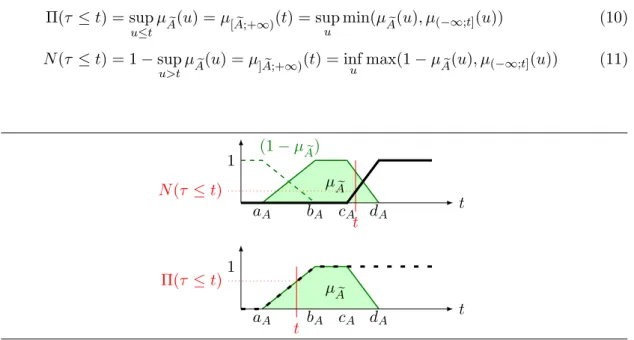
Let τ be a variable in the fuzzy interval eA and t be a real value. To measure the truth of the event τ ≤ t, equivalent to τ ∈ (−∞; t], we need the couple Π(τ ≤ t) and N (τ ≤ t) representing the fact that τ ≤ t is respectively possibly true and necessarily true (Fig. 2). Thus:
Π(τ ≤ t) = sup
u≤t
µ
e
A(u) = µ[ eA;+∞)(t) = sup u min(µ e A(u), µ(−∞;t](u)) (10) N (τ ≤ t) = 1 − sup u>t
µAe(u) = µ] eA;+∞)(t) = inf
u max(1 − µAe(u), µ(−∞;t](u)) (11)
1 aA bA cA dA t Π(τ ≤ t) µ e A t 1 aA bA cA dA t N (τ ≤ t) µAe (1 − µAe) t
Figure 2. Possibility and Necessity of τ ≤ t with τ ∈ eA.
Consequently, let τ and σ to be two variables in respectively fuzzy intervals eA and e
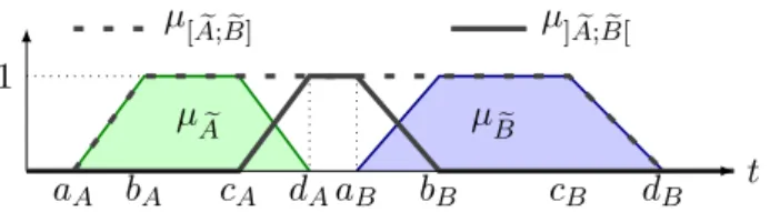
B, and t to be a real value. Based on the aforementioned possibility theory, we define a useful measure corresponding to the truth of the event ”t between τ and σ” by the couple Π(τ ≤ t ≤ σ) and N (τ ≤ t ≤ σ):
Π(τ ≤ t ≤ σ) = µ[ eA; eB](t) = µ[ eA;+∞)∩(−∞; eB](t) = min(µ[ eA;+∞)(t), µ(−∞; eB](t))
= min[sup
u
min(µ
e
A(u), µ(−∞;τ ](u)), sup v
min(µ
e
and
N (τ ≤ t ≤ σ) = µ] eA; eB[(t) = µ] eA;+∞)∩(−∞; eB[(t) = min(µ] eA;+∞)(t), µ(−∞; eB[(t))
= min[inf
u max(1 − µAe(u), µ(−∞;τ ](u)), infv max(1 − µBe(v), µ[τ ;+∞)(v)))]
(13) 1 aA bA cA dAaB bB cB dB µ e A µBe µ[ eA; eB] µ] eA; eB[ t
Figure 3. Necessity and possibility of t being between eA and eB.
Figure 3 presents the possibility and necessity membership functions for an event t to be between fuzzy intervals eA and eB.
3.3. Fuzzy Planning: State of the art
Since the early 90s, fuzzy logic became a very promising mathematical approach to mod-elling planning and scheduling problem characterized by uncertainty and imprecision.
We distinguish between production and project planning although they have some similarities. The Critical Path Method is one of the project planning specificities. It is based on two successive steps; a forward propagation to determine the earliest start and finish dates (and consequently the project duration and the free floats), and a backward propagation for the latest start and finish dates (and the total floats). In the fuzzy case, forward propagation is done using fuzzy arithmetic, leading to fuzzy earliest dates and a fuzzy end-of-project event. Unfortunately, backward propagation is no longer applicable because uncertainty would be taken into account twice. Dubois et al. (2003) show that the boundaries of some fuzzy parameters like the tasks’ latest dates and floats are reached in extreme configurations. Fortin et al. (2005) justify the problem complexity and propose some algorithms to calculate the tasks’ latest dates and floats. These parameters shall be used later to make decision on project delivering date on tactical level and deal with capacity problem on operational level of planning.
The study of a fuzzy model of resource-constrained project scheduling has been initi-ated in Hapke et al. (1994), and Hapke and Slowinski (1996). Many techniques partic-ularly the serial and parallel scheduling schemes (Hapke and Slowinski 1996), and the resource levelling technique (Leu et al. 1999) were generalized to fuzzy parameters. We refer readers to the volume edited by Slowinski and Hapke (2000) that gathers important work in fuzzy scheduling.
Applications of fuzzy logic to production planning is not widely used; a fuzzy mod-elling of delivery dates and of the resource capacities has for instance been suggested in Watanabe (1990), whereas imprecise operation durations and preferences at tactical level of production are considered in Inuiguchi et al. (1994). In Fargier and Thierry (2000) a fuzzy representation of imprecise ordered quantities is proposed. Recently in Grabot et al. (2005), a fuzzy MRP is provided based on the formalism of possibility distributions described in (Dubois and Prade 1988a). In tactical project planning, Masmoudi et al.
(2011) proposed a Simulated Annealing to solve the fuzzy capacity planning problem by providing a robust solution, hence several fuzzy robustness expressions are provided.
4. Modelling tactical plan
Without loss of generality, a multiple project capacity planning problem can be modelled as a single project capacity planning problem. This single project contains all macro-tasks from all projects. A tactical planning (RCCP) consists of allocating macro-tasks’ portions of work contents to time periods (e.g. 50 hours in period 3, 100 hours in period 4) in order to determine required capacity and reliable projects release and due dates.
The PUMA helicopter HMV, for example, contains about 18 macro-tasks and lasts about 6 months. Hence, the planning horizon for a helicopter maintenance is set to 12 months in order to cover the overall delay of a project. This situation can be compared to engineering-to-order (ETO) in manufacturing (Hans 2001).
In tactical level of planning, uncertainty is present in macro-tasks work contents as confirmed in (Elmaghraby 2002). In literature, few works deal with uncertainty in tactical planning using discrete stochastic distributions (Wullink 2005). Here, uncertainties in work contents are modelled with fuzzy numbers which presents a new contribution in project planning under uncertainty.
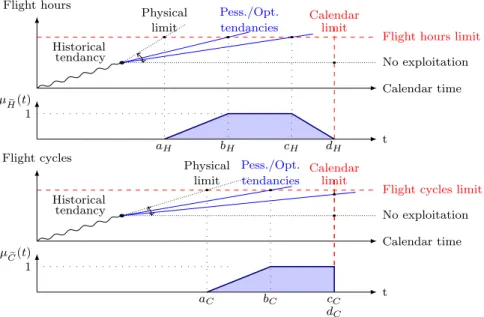
4.1. Modelling project release date
Figure 4 presents an example of an equipment inspection date determination from he-licopter exploitation assumptions, calendar limits and flight hours (top) or flight cycle (bottom) limits, for example 30000 hours or 15000 cycles by 10 years. From the update, flight hours evolve in a range going from no exploitation to the physical limits of the aircraft, through pessimistic and optimistic exploitation values. Intersections of these lines with calendar and flight hours limits define the four points aH, bH, cH and dH of
the trapezoidal fuzzy number eH, inspection date according to the flight hours. It is the same for flight cycles.
For a single equipment, the fuzzy inspection date is the minimum between fuzzy dates involved by flight hours ( eH) and cycles limits ( eC) (min( eH, eC), see section 3.1).
The fuzzy release date of the HMV is the fuzzy minimum of the inspection dates of critical equipments listed in the maintenance program, and of the helicopter itself. The uncertainty in this date decreases along the time, as information on actual exploitation increases.
The release and due dates are fixed 6 to 8 weeks ahead after a negotiation between the MRO and the customer (helicopter’s owner). Hence, a deterministic value of the release date is chosen with a certain risk among the possible values of the aforementioned fuzzy release date. Consequently, all tasks’ release and due dates are calculated using the deterministic Critical Path Method technique.
4.2. Fuzzy macro-task’s work content
At tactical level, uncertainty in macro task work content is mainly due to unexpected corrective maintenance. These additional tasks (work and delays) can represent one third to one half of the total project workload. They generally appear during the structural inspection macro tasks, but the whole project is impacted.
Calendar time Flight hours
Flight hours limit Calendar limit Historical tendancy Physical limit Pess./Opt. tendancies No exploitation µ e H(t) 1 t aH bH cH dH Calendar time Flight cycles
Flight cycles limit Calendar limit Historical tendancy Physical limit Pess./Opt. tendancies No exploitation µ e C(t) 1 t aC bC cC dC
Figure 4. Fuzzy inspection release date
Procurement for corrective maintenance may introduce delays in the planning. As the equipments to be purchased are not known before inspection, we consider different sce-narios: the equipment is available on site; or at an European supplier; or at a foreign supplier; or it may be found after some research; or it is obsolete and must be man-ufactured again. According to the information on the helicopter (age of the aircraft, conditions of use, etc...), some scenarios can be discarded from the beginning (e.g. new helicopter ⇒ no obsolescence) and others at the end of the major inspection tasks and hence macro-tasks’ workloads are refined.
macro-tasks’ work content are established by asking experts. Rommelfanger (1990) pro-poses a 6-point fuzzy number to represent the expert knowledge. In this work, however, we will still consider 4-point fuzzy numbers within a trapezoidal profile.
Each macro-task’s work content is divided into portions that are allocated to the time periods between the macro-task’s starting and finishing dates. Let consider a macro-task
e
A with a fuzzy work content PAe = (120, 180, 240, 300) present between period 3 and period 5. One third of the work content corresponds to resource type 1(υA1e = 1/3) and two third corresponds to resource type 2(υ
e
A2= 2/3). We choose to carry out the three
quarters of the macro-task eA at period 3(YA3e = 3/4) and the other quarter at period 4(Y
e
A4= 1/4). Table 1 shows the macro-task and its different work content portions.
Table 1. Macrotask Resource portions
Macro-task Resource type Period 3 Period 4
A 1 (30,45,60,75) (10,15,20,25)
4.3. Fuzzy workload plan
A feasible tactical plan respects all technological restrictions (precedence relations, macro-tasks durations and macro-tasks release, and due dates). We consider a set of macro-tasks (index j ∈ 1, . . . , n) with corresponding work content denoted pj and
min-imum duration denoted ωj. To perform a macro-task, several resource groups (index
i ∈ 1, . . . , I) are needed. The fraction of macro-task work content pj performed by
re-source group i is denoted υji, so that Piυji = 1 ∀j. We consider a planning horizon
discretized into T periods (index t). Variable Yjt represents the fraction of the work
content of task j executed in period t.
A macro-tasks plan aj (j = 1, . . . , n) specifies for each macro-task j the periods in
which it is allowed to be performed. A macro-task plan aj is a vector of 0-1 values ajt
(t = 0, . . . , T ) where ajt = 1 if macro-task j is allowed to be performed in period t, 0
otherwise. A feasible macro-task plan respects release and due dates of macro-task as well as precedence constraints. Hence, to ensure consistency, variables Yjtcan be greater than
0 if and only if ajt = 1. The vector Yj of variables Yjt, t = 0, . . . , T is called macro-task
schedule. Let Pjt = pj.Yjt be the amount of the work content (in hours) of macro-task j
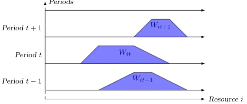
to be executed in period t (t = 0, . . . , T ). A tactical plan is defined by parameters fWit
=P
jepjυjiYjt corresponding to the total workload by resource group i (i ∈ 1, . . . , I) to be executed in period t (t = 0, . . . , T ) (Figure 5) while fWitare fuzzy numbers calculated
using formula (1) and (7) (fWit= (aWit, bWit, cWit, dWit)).
Periods
Resource i
Period t − 1 Wit−1
Period t Wit
Period t + 1 Wit+1
Figure 5. Partial fuzzy workload plan
4.4. Decision making on fuzzy tactical planing
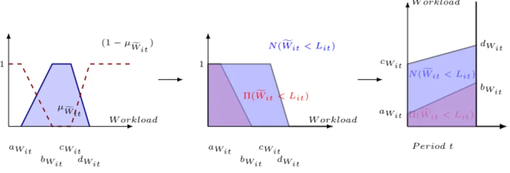
Let Lit to be the capacity limit of the resource i at period t = 0, . . . , T . To check if the
fuzzy workload exceeds the capacity limit or not, we consider the possibilistic approach. In fact, to measure the truth of the event fWit < Lit, we need the couple Π(fWit < Lit)
and N (fWit< Lit) (see section 3.2).
In Figure 6, we show the way to represent a fuzzy load by period using the necessity and possibility measures. This representation is similar to the one proposed by Grabot et al. (2005) to model uncertainty in orders in MRP method.
Let Nit and Πit to be the values of the workload membership function intersection
with the capacity limits: ∀i, t Nit = N (fWit < Lit) and Πit = Π(fWit < Lit) (∀i, t) with
1 aWit bWit cWit dWit µ f Wit (1 − µ f Wit) W orkload 1 aWit bWit cWit dWit Π(fWit< Lit) N (fWit< Lit) W orkload W orkload P eriod t aWit bWit Π(fWit< Lit) cWit dWit N (fWit< Lit)
Figure 6. How to get a fuzzy load by period using the Necessity and possibility measures.
Πit are calculated as follows:
Nit= 0 ifLit < cWit Lit−cWit
dWit−cWit if Lit∈ [cWit, dWit]
1 ifLit > dWit (14) Πit= 0 if Lit < aWit Lit−aWit
bWit−aWit if Lit ∈ [aWit, bWit]
1 if Lit > bWit
(15)
Note that Crit= Nit+ Πit(∀i, t) is called the credibility of workload fWit being under the
limit of capacity Lit. These variables are to minimize while dealing with optimization on
capacity planning problem (Masmoudi et al. 2011).
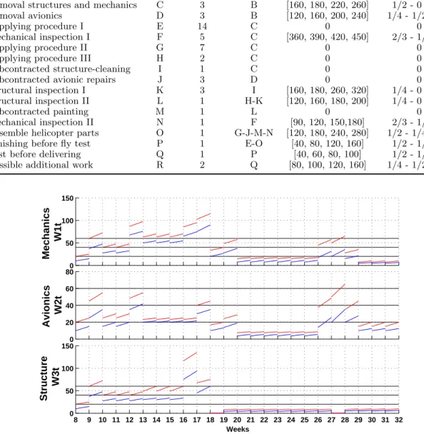
4.5. A Helicopter maintenance case study
In the helicopter maintenance center, three main human resources are needed to perform HMVs: mechanic experts (i = 1), avionic experts (i = 2) and structure experts (i = 3). Table 2 contains data of a real HMV project.
Different flexible capacity levels are considered when dealing with tactical planning: regular capacity, overtime capacity, hired capacity and subcontracted capacity.
In this paper, we do not deal with optimization problem. Hence, Figure 7 shows the earliest plan while resource constraint are not considered. The example of earliest plan corresponds to a uniform distribution of macro-task work content : Yjt=1/ωj for all
t ∈ [Esj, Efj] where Esj is the earliest starting date and Efj the earliest finishing date.
We consider the example where the regular capacity limit, the overtime capacity limit, and the hiring capacity limit are constant; and equal to 20, 40 and 60 hours, respectively. While dealing with optimization, the main objective within a resource driven approach will be to minimize the overcapacity (overtime, hired, and subcontracted capacities) (Masmoudi et al. 2011).
Once a tactical plan is provided, we deal with operational plan. Interaction between the two levels is not discussed in this study.
Table 2. Example of a real HMV project.
Task Name Task Duration Pred. Work contents Resource fraction i=(1-2-3)
Release date A 8 - 0 0
First check B 1 A [60, 90, 120, 150] 1/3 - 1/3 - 1/3
Removal structures and mechanics C 3 B [160, 180, 220, 260] 1/2 - 0 - 1/2
Removal avionics D 3 B [120, 160, 200, 240] 1/4 - 1/2 - 1/4
Supplying procedure I E 14 C 0 0
Mechanical inspection I F 5 C [360, 390, 420, 450] 2/3 - 1/3 - 0
Supplying procedure II G 7 C 0 0
Supplying procedure III H 2 C 0 0
Subcontracted structure-cleaning I 1 C 0 0
Subcontracted avionic repairs J 3 D 0 0
Structural inspection I K 3 I [160, 180, 260, 320] 1/4 - 0 - 3/4 Structural inspection II L 1 H-K [120, 160, 180, 200] 1/4 - 0 - 3/4
Subcontracted painting M 1 L 0 0
Mechanical inspection II N 1 F [90, 120, 150,180] 2/3 - 1/3 - 0 Assemble helicopter parts O 1 G-J-M-N [120, 180, 240, 280] 1/2 - 1/4 - 1/4 Finishing before fly test P 1 E-O [40, 80, 120, 160] 1/2 - 1/2 - 0 Test before delivering Q 1 P [40, 60, 80, 100] 1/2 - 1/2 - 0 Possible additional work R 2 Q [80, 100, 120, 160] 1/4 - 1/2 - 1/4
0 50 100 150 Weeks Mechanics W1t 0 20 40 60 80 Avionics W2t 8 9 10 11 12 13 14 15 16 17 18 19 20 21 22 23 24 25 26 27 28 29 30 31 32 0 50 100 150 Structure W3t
Figure 7. Fuzzy workload plan for a HMV.
5. Modelling operational plan
In operational level of planning we handle small tasks, hence macro-tasks from tactical level are decomposed into elementary tasks. Tasks’ durations are established by asking experts. To represent the expert knowledge at operational level of planning, we consider 4-point trapezoidal numbers. Uncertainty in tasks durations is mainly due to the skills of operators assigned to the tasks, the unexpected absence of resources (operators and/or facilities), and frequent small updates coming from manufacturers and authorities.
Here we propose to establish a workload plan based on the fuzzy starting and finishing dates of tasks. To achieve this aim, we apply the possibility theory (Zadeh 1978) in order
to represent the presence of a task in a period and deduce the distribution of resource required by a task, and the total workload for all tasks. Starting times and finishing times of all tasks are defined by applying fuzzy PERT technique. In literature, several deterministic resource workload plans are established by applying alpha-cuts (Hapke and Slowinski 1996, Leu et al. 1999) on the fuzzy starting and finishing dates. We get a couple of deterministic workload plans (pessimistic and optimistic) for each value of alpha-cut in [0, 1]. Instead of applying alpha-cuts on a fuzzy Gantt to get deterministic resource plans, in this section, we provide a new technique to deal with fuzzy resource planning where both Gantt and workload plan are considered fuzzy.
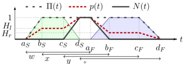
5.1. Task presence domain
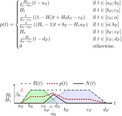
Let eS(aS, bS, cS, dS) be the fuzzy earliest start date of a task T , eF (aF, bF, cF, dF) its
earliest finish date and eD(w, x, y, z) its duration. Relations between these values is eF = e
S + eD.
Using fuzzy arithmetic, we can define ] eS; eF [ (resp. [ eS; eF ]), the domain where the task T presence is necessarily (resp. possibly) true. They represent the truth of the event ”t between the starting and the finishing date of T ”. Associated membership functions, µ] eS; eF [(t) and µ[ eS; eF ](t) are respectively denoted N (t) and Π(t)(Figure 8).
1 aS bS cS dS Hr Hl aF bF cF dF w x y z Π(t) p(t) N (t) t
Figure 8. Presence of a task: No overlap configuration.
In the configuration of Figure 8, we can identify the following intervals of possibility and necessity: [dS; aF] : Π = 1 N = 1 [cS; dS] and [aF; bF] : Π = 1 N ≥ 0 [bS; cS] and [bF; cF] : Π = 1 N = 0 [aS; bS] and [cF; dF] : Π ≥ 0 N = 0 [0; aS] and [dF; +∞[ : Π = 0 N = 0
Then we characterize the probability of task T presence as a distribution p(t) situated between the possibility and the necessity profiles: N (t) ≤ p(t) ≤ Π(t).
We propose a parametric piecewise linear distribution to represent the probability of presence of the task (dashed line on Figure 8). It will be used to establish resource
requirement. This distribution corresponds to the intervals of possibility and necessity: p(t) = Hl bS−aS(t − aS) if t ∈ [aS; bS] Hl if t ∈ [bS; cS] 1 dS−cS ((1 − Hl)t + HldS− cS) if t ∈ [cS; dS] 1 if t ∈ [dS; aF] 1 bF−aF ((Hr− 1)t + bF − HraF) if t ∈ [aF; bF] Hr if t ∈ [bF; cF] −Hr dF−cF(t − dF) if t ∈ [cF; dF] 0 otherwise, (16)
where parameters Hl and Hr, varying from 0 to 1, makes profile p(t) evolve from N (t)
(Hl = Hr= 0) to Π(t) (Hl= Hr= 1).
Figure 8 presented a configuration without overlap between fuzzy start and finish dates (dS ≤ aF). Two more configurations exist (Figure 9 and Figure 10): small overlap
(dS > aF and cS ≤ bF) and large overlap (cS > bF). Note that the maximal necessity
value is respectively lower than 1 for small overlap and equal to 0 for large overlap. In the same way that for the first configuration, a parametric piecewise linear distribution can be defined to represent the probability of task presence.
For the small overlap configuration, the distribution is (dashed line on Figure 9):
p(t) = Hl bS−aS(t − aS) if t ∈ [aS; bS] Hl if t ∈ [bS; cS] 1 dS−cS ((1 − Hl)t + HldS− cS) if t ∈ [cS; α] 1 bF−aF ((Hr− 1)t + bF − HraF) if t ∈ [α; bF] Hr if t ∈ [bF; cF] −Hr dF−cF(t − dF) if t ∈ [cF; dF] 0 otherwise. (17) aS bS cS dS aF bF cF dF β β0 α0 α Hr Hl Π(t) p(t) N (t) t
Figure 9. Presence of a task: small overlap configuration.
α = (bF − aF)(HldS− cS) + (dS− cS)(HraF − bF) (bF − aF)(Hl− 1) + (dS− cS)(Hr− 1) (18) β = (bF − HraF)(Hl− 1) + (HldS− cS)(Hr− 1) (bF − aF)(Hl− 1) + (dS− cS)(Hr− 1) (19)
And particularly while Hl = Hr= H:
α = α0 = ds.bf − af.cs (bf − cs) + (ds− af) (20) β = (bf− cs) + H(ds− af) (bf − cs) + (ds− af) (21)
The value β varies in a range [β0, 1] and the value α varies in a range [aF, dS] along with
parameters Hl and Hr. 1 aS bS cS dS aF bF cF dF Hr Hl t
Figure 10. Presence of a task: large overlap configuration.
For the large overlap configuration, the distribution is (dashed line on Figure 10):
p(t) = Hl bS−aS(t − aS) if t ∈ [aS; bS] Hl if t ∈ [bS; bF] 1 bF−cS((Hl− Hr)t + HrbF − HlcS) if t ∈ [bF; cS] Hr if t ∈ [cS; cF] −Hr dF−cF(t − dF) if t ∈ [cF; dF] 0 otherwise. (22)
5.2. Fuzzy task workload
The establishment of a relevant resource usage profile for a task with fuzzy dates and duration is difficult. Most of the time, the problem parameters are fixed in order to obtain a deterministic configuration. This leads to a scenario approach (Hapke and Slowinski 1996, Wullink et al. 2004) where various significant scenarios may be compared in a decision process: lower and upper bounds, most plausible configuration, etc...
In this paper we propose to build a task resource usage profile in a way that keeps track of uncertainty in start and finish dates. Hence, the profile reflects the whole pos-sible time interval while giving a plaupos-sible repartition of the workload according to the duration parameter value. To achieve this aim, the resource usage profiles are defined as a projection of the task presence distributions onto the workload space.
1 aS bS cS dS Hr Hl aF bF cF dF Π(t) p(t) N (t) t r aS bS cF dF t r cS dS aF bF t 1 β0 aS bS cS dS aF bF cF dF Π(t) p(t) N (t) t r aS bS cF dF t rβ0 cS bF t 1 aS bS cSdS aFbF cF dF Π(t) p(t) N (t) t r aS bS cF dF t t
Figure 11. Resource profiles: projection of possibility (middle) and necessity (bottom) distribu-tions.
Let us consider first the case with no overlap between eS and eF (Figure 11, top, left). Suppose that the resource requirement of the task is r. Resource workload then lies in [r.w; r.z], according to the task duration.
Consequently, for any duration between w and z, the resource usage profile is repre-sented by a projection of the task presence probability distribution p(t). The link between the task duration and the profile, for a duration D, is given by the following formula:
r.D = Z +∞ 0 r.p(t)dt = r.Hl( dS− bS 2 + cS− aS 2 ) + r.Hr( cF − aF 2 + dF − bF 2 ) + r.( aF − dS 2 + bF − cS 2 ) (23)
and for the particular case where (Hl= Hr = H):
r.D = Z +∞ 0 r.p(t)dt = r.H(dF − aS 2 + cF − bS 2 ) + r.(1 − H)( aF − dS 2 + bF − cS 2 ) (24)
For the maximal workload, the area covered by the projection of the possibility distri-bution is:
r.DΠ= r.(dF − aS+ cF − bS)/2 (25)
For the minimal workload, the area covered by the projection of the necessity distribution is:
r.DN = r.(bF − cS+ aF − dS)/2 (26)
In case of small overlap(Figure 11, top, middle), the link between the task duration and the profile, for a duration D, is given by the following formula:
r.D = Z +∞ 0 r.p(t)dt = r.Hl( cS+ α 2 − aS+ bS 2 ) + r.Hr( dF + cF 2 − α + bF 2 ) + r.β( bF − cS 2 ) (27)
The area of the projected necessity distribution is:
r.DN = r.β0 bF − cS 2 = r (bF − cS)2 2(dS− aF + bF − cS) (28) where: β0= (bf − cs) (bf− cs) + (ds− af) (29)
In the configuration with large overlap, the maximal resource profile is treated like other configurations, because the possibility distributions are the same. On the other hand, the minimal resource profile is treated differently.
In case of large overlap(Figure 11, top, right), the link between the task duration and the profile, for a duration D, is given by the following formula:
r.D = Z +∞ 0 r.p(t)dt = r.Hl( cS+ bF 2 − aS+ bS 2 ) + r.Hr( dF + cF 2 − cS+ bF 2 )) (30)
and for the particular case where (Hl= Hr = H):
r.D = Z +∞ 0 r.p(t)dt = r.H(dF + cF 2 − aS+ bS 2 ) (31)
The necessity profile is null (N (t) = 0 ∀t), thus r.DN = 0.
For different configurations, the particular cases where the necessity distribution is greater than the minimal workload r.w and the cases where the possibility distribution is lower than the maximal workload r.z are treated in details in Masmoudi and Ha¨ıt (2010).
5.3. Project workload
The workload depends on the tasks’ durations. Moreover, the fuzzy task workload gives an idea about resources needed according to uncertainty in task starting and finishing dates.
During capacity planning phase, a workload plan is drawn for each resource type in-volved in the maintenance operations in order to identify overloaded resources. If the tasks were independent, the sum of their workload profiles would give the overall work-load plan. However, when considering a precedence constraint between two tasks, their workload profiles may not overlap because they can not be performed simultaneously.
Let us consider two tasks A and B so that A precedes B. Their resource consumptions are denoted rA and rB. We assume that the start date of B is equal to the finish date
of A (e.g. in case of forward earliest dates calculation). This means that between the start date of A and the finish date of B, an activity will occur successively induced by A then B. So between the necessity peaks of A and B, we can affirm that an activity will necessarily occur, induced by A or B. This necessary presence of A or B is projected onto the resource load space using the minimal resource requirement min(rA, rB), associated
to pseudo task A ∨ B starting at eSA and finishing at eFB (Figure 12). The projected
necessity and possibility load profiles of the sequence A → B are defined as follow:
LN (A→B)(t) = max(rA.NA(t), rB.NB(t), min(rA, rB).NA∨B(t)) (32)
LΠ(A→B)(t) = max(rA.ΠA(t), rB.ΠB(t)) (33)
The probability workload profile is more complex to define. A constructive way can be provided; firstly the distribution of A is defined and then the distribution of B is deduced respecting resources and precedence constraints. Let us consider A without predecessors. Hence, we can assign to A its symmetric distribution while HAl = HAr = HA. For B we
apply the following checks:
if rBHB> max(rB, rA) − rAHAr then
Hl
B= (max(rB, rA) − rAHAr)/rB
else if rBHB < min(rB, rA).N (A ∨ B) − rAHAr then
HBl = (min(rB, rA).N (A ∨ B) − rAHAr)/rB
else HBl = HB
HBr = f (HBl, DB)
Where DB is the duration of B, f is a function deduced from (23), (27), and (30), and
Hj is the parameter value of task j distribution while considering HBl = HBr.
Once probabilistic distributions of A and B are defined respecting resource and prece-dence constraints, the sum of the two distributions corresponds to the total probabilistic workload:
LP (A→B)(t) = rA.PA(t) + rB.PB(t) (34)
Figure 12 shows the workload while rA= 2, and rB = 1. Integration of these profiles
considering updates made by the aforementioned formulae gives the total workload. The aforementioned approach can be easily generalized to multi-tasks within the frame of a fuzzy scheduling technique. For example, Hapke and Slowinski (1996) provide a generalization of parallel SGS to fuzzy area. They use weak and strong fuzzy inequalities to compare fuzzy numbers and provide a direct tasks sequence respecting both resources and precedence constraints. Let S (index j = 1..S) to be the set of tasks to schedule. Within a loop, we calculate each task’s j distribution parameters (Hjl then Hjr) task by
task within a new parallel SGS technique for example based on the aforementioned fuzzy workload modelling: 2 t PA(t) 1 t PB(t) 1 t N (A ∨ B)Π(A ∨ B) 1 2 t LΠ(A→B)(t) LP (A→B)(t) LN (A→B)(t)
Figure 12. Fuzzy continuous workload plan.
Choose a priority rule,
Initialize fEsj; the earliest starting time of task j (∀j), using the CPM technique,
Initializeet =et0; the begin of the scheduling horizon (e.g.et = 0), Initialize the total resources availabilities at all scheduling periods, Repeat
Compose the set Av(et) of available tasks atet
for each j from Av(et), in the order of the priority list do begin
calculate the corresponding symmetric probabilistic distribution Pj
if the symmetric probabilistic distribution Pj does not fit period by period the
resources availabilities then
calculate a new Pj with a asymmetric shape considering the minimum possible
value of the left parameter (Hl j)
if the configuration Pj fits the resource availabilities then
begin
schedule j with corresponding starting and finishing dates,
integrate the distribution Pj into the workload plan and update the total
resources availabilities,
update the earliest starting time of all successors of j, end
end end
if all tasks from Av(et) are scheduled then e
t = max(et, el(et)) elseet = max(et, at+ 1) Until all tasks are scheduled where:
The considered defuzzification technique is the mean value provided by (Dubois and Prade 1987). Hence, Let t to be the mean value ofet thus t = (at+ bt+ ct+ dt)/4.
Av(et) is the set of tasks whose defuzzification value of Earliest Starting time Es are less or equal to the defuzzification value ofet (Esj ≤ t, ∀j ∈ Av(et)).
el(et) is the least value among the earliest starting times of tasks from A(et) and the finishing times of tasks from S(et).
A(et) is the set of tasks that are not yet scheduled and whose immediate predecessors have been completed byet.
S(et) is the set of tasks present inet; a task j is considered present inet when Sj ≤ t ≤ Fj(Sj and Fj are the defuzzifications of starting and finishing time of j, respectively.
5.4. A Helicopter maintenance case study
Let us consider the mechanical inspection (macro-tasks F and N in Table 2) from PUMA helicopter HMV.
The major mechanical parts to check within the mechanical inspection are:
Table 3. Real mechanical tasks from a PUMA HMV.
Part name Taks Id Id Pred. Experts Equipments Duration (days)
Main Rotor
Put off Muff 1 - 1 - [0.5, 0.7, 1, 1.5]
Put off bearings 2 1 1 - [1, 1.2, 1.4, 1.6]
Put off flexible components 3 - 1 - [0.1, 0.13, 0.17, 0.2]
Clean 4 2-3 1 Cleaning machine [1, 1.2, 1.4, 1.5]
Non-destructive test 5 4 1 Testing equipment [0.2, 0.3, 0.5, 0.6]
Assemble components 6 5 1 - [1, 1.2, 1.4, 1.5]
Check water-tightness 7 6 1 - [0.2, 0.3, 0.4, 0.5]
Touch up paint 8 7 1 - [0.1, 0.13, 0.17, 0.2]
Tight screws 9 8 1 - [0.3, 0.5, 0.6, 0.7]
Propeller
Put off axial compressor 10 - 1 - [1.2, 1.5, 1.8, 2]
Put off centrifugal compressor 11 10 1 - [1.5, 1.6, 1.8, 2]
Purchase 12 10 0 - [0, 1, 2, 4]
Put off turbine 13 - 1 - [0.5, 0.7, 0.8, 1]
Clean 14 11-13 1 Cleaning machine [0.2, 0.4, 0.5, 0.6]
Non-destructive test 15 14 1 Testing equipment [0.2, 0.3, 0.4, 0.5]
Assemble components 16 12-15 1 - [2, 2.2, 2.8, 3.2]
Touch up paint 17 16 1 - [0.1, 0.13, 0.16, 0.2]
Tight screws 18 17 1 - [0.12, 0.17, 0.2, 0.3]
Test 19 18 1 Test Bench [0.12, 0.17, 0.2, 0.23]
Hydraulic System
Evacuate oil 20 - 2 - [0.1, 0.13, 0.16, 0.2]
Put off servos 21 20 2 - [0.6, 0.7, 0.8, 1]
Clean 22 21 1 Cleaning machine [0.2, 0.3, 0.4, 0.6]
Non-destructive test 23 22 1 Testing equipment [0.2, 0.3, 0.4, 0.6] Assemble then remove joints 24 23 2 - [0.8, 1, 1.2, 1.4]
Test 25 24 1 Test Bench [0.1, 0.13, 0.16, 0.2]
Tight screws 26 25 2 - [0.1, 0.13, 0.16, 0.2]
• Main Rotor: The work is carried out by 1 expert during 35 to 70 hours. • Tail Rotor: The work is carried out by 1 expert during 17 to 35 hours.
• Main Gear Box: The work is carried out by 1 to 2 experts during 70 to 105 hours. It is often subcontracted to the manufacturer.
• Propeller: The work is carried out by 1 expert during 70 to 105 hours.
• Hydraulic System: The work is carried out by 1 to 2 experts during 18 to 35 hours. Each part inspection can be considered as a small project containing several tasks subject to precedence constraints. The MRO capacity (technicians and equipments) is
limited thus resources will be shared by all projects. Hence, the problem is to schedule small projects respecting precedence constraints and workshop resources constraints.
For each task j, we need to transform the work content pj into a duration Dj based
on 35-hour working week and the number of operators nj assigned to j: Dj = pj/35 ∗ nj.
To show the scheduling problem in MRO within a simple example, we consider one helicopter and three parts to check which are the Main Rotor, the Propeller and the Hydraulic System gear. We consider that our experts have the necessary qualifications to inspect different parts. Table 3 contains the corresponding data.
Let us take the case where 3 operators are available at one time, only 1 test bench, 1 Non-destructive testing equipment, and 1 cleaning machine exist in the workshop. Apply-ing the parallel SGS of Hapke and Slowinski (1996) with the consideration of the Shortest Processing Time(SPT) rule, for example, and an update of resources availabilities based on algorithm specified in section 5.3, we get a feasible scheduling with corresponding continuous fuzzy workload (see Figure 13).
Fuzzy Gantt & Fuzzy Workload
(Task) 1 2 3 4 5 6 7 8 9 10 11 12 13 14 15 16 17 18 19 20 21 22 23 24 25 26 3 2 1 starting time finishing time distribution r.P(t) 0 1 2 3 4 5 6 7 8 9 10 11 12 Days Experts (number) workload
Figure 13. A partial schedule of the HMV mechanical inspection
Several rules are defined in Masmoudi et al. (2011), while task durations are fuzzy, to solve multi-project and multi-resource scheduling problem. Based on the aforementioned fuzzy resource modelling, we can generalize many existing scheduling techniques to deal with optimization goals. However, it is not the objective of this paper.
6. Conclusion
In this paper, we have presented a fuzzy model for project scheduling and planning problems. A method to establish a resource workload is proposed for both tactical and operational levels of planning. Provided models are applied to the helicopter mainte-nance domain. Based on these modelling approaches, some recent papers provide a gen-eralization of several scheduling heuristics to fuzzy parameters; a Genetic Algorithm is generalized to solve Fuzzy Resource Levelling Problem (Masmoudi and Ha¨ıt 2011b), a Parallel SGS is generalized to solve Fuzzy RCSPS problem (Masmoudi and Ha¨ıt 2011a), and a Simulated Annealing is generalized to solve Fuzzy RCCP problem (Masmoudi et al. 2011). Future work will focus on providing exhaustive list of configurations within different possible fuzzy profiles (rectangular, triangular, exponential...). The comparison of our fuzzy approaches (models and solving techniques) to existing stochastic ones is under study. It will be interesting to study the link between the tactical level and the operational level. The afore developed fuzzy techniques will be included into a Decisional Support System to manage a MRO center.
References
Chen, S. and Hwang, C., 1992. Fuzzy multiple attribute decision making: Methods and applications. Fuzzy sets.
Chen, S.Q., 2000. Comparing probabilistic and fuzzy et approaches for designing in the presence of uncertainty. Thesis (PhD). Virginia Polytechnic Institute and State University, Blacksburg, Virginia.
Dubois, D., Fargier, H., and Galvagnon, V., 2003. On latest starting times and floats in activity networks with ill-known durations. European Journal of Operational Re-search, 147 (2), 266–280.
Dubois, D. and Prade, H., 1987. The mean value of a fuzzy number. Fuzzy Sets and Systems, 24 (3), 279–300.
Dubois, D. and Prade, H., 1988a. Possibility theory: an approach to computerized pro-cessing of uncertainly. New York: Plenum Press.
Dubois, D. and Prade, H., 1988b. Possibility theory: an approach to computerized pro-cessing of uncertainty. International Journal of General Systems.
Elmaghraby, S.E., 2002. Contribution to the round table discussion on new challenges in project scheduling. In: PMS Conference, April 3-5., Valencia, Spain.
Fargier, H. and Thierry, C., 2000. The use of possibilistic decision theory in manufacturing planning and control, Recent results in Fuzzy Master Production. In: R. Slowinski and M. Hapke, eds. Scheduling in Scheduling under Fuzziness. Springer-Verlag, 45– 59.
Fortin, J., et al., 2005. Interval Analysis in Scheduling. In: P. van Beek, ed. Principles and Practice of Constraint Programming - CP 2005., Vol. 3709 of Lecture Notes in Computer Science Springer Berlin / Heidelberg, 226–240.
Gademann, N. and Schutten, M., 2005. Linear-programming-based heuristics for project capacity planning. IIE Transactions, 37, 153–165.
Grabot, B., et al., 2005. Integration of Uncertain and Imprecise Orders in the MRP Method. International Journal of Intelligent Manufacturing, 16 (2), 215–234. Guiffrida, A.L. and Nagi, R., 1998. Fuzzy set theory applications in production
39–56.
Hahn, R.A. and Newman, A.M., 2008. Scheduling United States Coast Guard helicopter deployment and maintenance at Clearwater Air Station, Florida. Computers and Operations Research, 35 (6), 1829–1843.
Hans, E.W., 2001. Resource Loading by Branch-and-Price Techniques. Thesis (PhD). Twente University Press, Enschede, Netherland.
Hans, E.W., et al., 2007. A hierarchical approach to multi-project planning under uncer-tainty. Omega, 35, 563–577.
Hapke, M., Jaszkiewicz, A., and Slowinski, R., 1994. Fuzzy project scheduling system for software development. Fuzzy Sets and Systems, 67 (1), 101–117.
Hapke, M. and Slowinski, R., 1996. Fuzzy priority heuristics for project scheduling. Fuzzy Sets and Systems, 83 (3), 291–299.
Inuiguchi, M., Sakawa, M., and Kume, Y., 1994. The usefulness of possibilistic pro-gramming in production planning problems. International Journal of Production Economics, 33 (1-3), 45–52.
Leu, S.S., Chen, A.T., and Yang, C.H., 1999. A Fuzzy Optimal Model for Construction Resource Leveling Scheduling. Canadian Journal of Civil Engineering, 26, 673–684. Masmoudi, M. and Ha¨ıt, A., 2010. A Tactical model under uncertainty for helicopter maintenance planning. In: the 8th ENIM IFAC International Conference of Modeling and Simulation, MOSIM’10, Vol. 3, May., Hammamet, Tunisia, 1837–1845.
Masmoudi, M. and Ha¨ıt, A., 2011a. Fuzzy capacity planning for an helicopter mainte-nance center. In: International Conference on Industrial Engineering and Systems Management, IESM’11, May., Metz, France.
Masmoudi, M. and Ha¨ıt, A., 2011b. A GA-based fuzzy resource leveling optimization for helicopter maintenance activity. In: the 7th conference of the European Society for Fuzzy Logic and Technology, EUSFLAT’11, July., Aix-Les-Bains, France.
Masmoudi, M., Hans, E., and Ha¨ıt, A., 2011. Fuzzy tactical project planning: Application to helicopter maintenance. In: the 16th IEEE International Conference on Emerging Technologies and Factory Automation ETFA’2011, September., Toulouse, France. Rommelfanger, H., 1990. FULPAL: An interactive method for solving
(multiobjec-tive) fuzzy linear programming problems. Lecture Notes in Computer Science, In: R. Slowinski and J. Teghem, eds. Stochastic versus Fuzzy Approaches to Multiobjec-tive Mathematical Programming under Uncertainty. Kluwer.
Sgaslink, A., Planning German Army Helicopter Maintenance And Mission Assignement. Master’s thesis, Naval Postgraduate School, California, 1994. .
Slowinski, R. and Hapke, M., 2000. Scheduling under Fuzziness. Physica-Verlag.
Watanabe, T., 1990. Job-shop Scheduling Using Fuzzy Logic in a Computer Integrated Manufacturing Environment. In: the 5th International Conference on Systems Re-search, Informatics and Cybernetics, August.
Wullink, G., 2005. Resource Loading Under Uncertainty. Thesis (PhD). Twente Univer-sity Press, Enschede, Netherland.
Wullink, G., et al., 2004. A scenario based approach for flexible resource loading under uncertainty. International Journal of Production Research, 42 (24), 5079–5098. Zadeh, L., 1965. Fuzzy sets. Information and Control, 8, 338–353.
Zadeh, L., 1978. Fuzzy sets as basis for a theory of possibility. Fuzzy sets and systems, 1, 3–28.