Disparity-compensated view synthesis for s3D content correction

HAL Id: hal-00787332

https://hal.archives-ouvertes.fr/hal-00787332v2

Submitted on 12 Feb 2013

HAL is a multi-disciplinary open access

archive for the deposit and dissemination of

sci-entific research documents, whether they are

pub-lished or not. The documents may come from

teaching and research institutions in France or

abroad, or from public or private research centers.

L’archive ouverte pluridisciplinaire HAL, est

destinée au dépôt et à la diffusion de documents

scientifiques de niveau recherche, publiés ou non,

émanant des établissements d’enseignement et de

recherche français ou étrangers, des laboratoires

publics ou privés.

Disparity-compensated view synthesis for s3D content

correction

Philippe Robert, Cédric Thébault, Pierre-Henri Conze

To cite this version:

Philippe Robert, Cédric Thébault, Pierre-Henri Conze. Disparity-compensated view synthesis for s3D

content correction. Stereoscopic Displays and Applications, Jan 2012, San Francisco, United States.

pp.8288-86. �hal-00787332v2�

Disparity-compensated view synthesis for s3D content correction

Philippe Robert

, Cédric Thébault

, Pierre-Henri Conze

Technicolor

INSA Rennes, IETR/UMR 6164, UEB

ABSTRACT

The production of stereoscopic 3D HD content is considerably increasing and experience in 2-view acquisition is in progress. High quality material to the audience is required but not always ensured, and correction of the stereo views may be required. This is done via disparity-compensated view synthesis. A robust method has been developed dealing with these acquisition problems that introduce discomfort (e.g hyperdivergence and hyperconvergence…) as well as those ones that may disrupt the correction itself (vertical disparity, color difference between views…). The method has three phases: a preprocessing in order to correct the stereo images and estimate features (e.g. disparity range…) over the sequence. The second (main) phase proceeds then to disparity estimation and view synthesis. Dual disparity estimation based on robust block-matching, discontinuity-preserving filtering, consistency and occlusion handling has been developed. Accurate view synthesis is carried out through disparity compensation. Disparity assessment has been introduced in order to detect and quantify errors. A post-processing deals with these errors as a fallback mode. The paper focuses on disparity estimation and view synthesis of HD images. Quality assessment of synthesized views on a large set of HD video data has proved the effectiveness of our method.

Keywords: Post-production, 2-view stereo correction, Disparity estimation, View synthesis, Quality assessment, Depth

Image Based Rendering, Free Viewpoint Video

1. INTRODUCTION

The production of stereoscopic 3D HD content is considerably increasing and experience in 2-view acquisition is in progress. While high quality material to the audience is required this is not always ensured. In particular, a set of problems require modifying the views in post-production. This is the case for example when camera hyperconvergence or hyperdivergence introduce discomfort. Furthermore, different viewing conditions (e.g. 3DTV, movie theater) require also to adapt the acquisition data via view modifications1. The correction or modification is carried out through virtual view synthesis to replace at least one of the original views.

In this production context, our work aims at providing high quality view synthesis. Then the objective is to develop accurate disparity estimation and view synthesis with minimized user assistance. This new Depth Image Based Rendering (DIBR) scheme is based on three main phases (Figure 1):

Stereo video pre-processing: existence of vertical disparity or color difference between images breaks a priori hypotheses the estimator relies on. Pre-processing is introduced to solve these issues as well as to estimate features (noise, disparity range…) over the stereo sequence to be used in the main phase.

Robust 1D disparity estimation and view synthesis:

a. Disparity estimation: this is an ill-posed problem as numerous cases of image content introduce ambiguity in disparity (occlusions, textureless areas, periodic structures, transparency, light reflections...). The objective is to satisfactorily solve most of the sequences via a robust algorithm. The method results from the combination of four constraints assigned to disparity: minimal correspondence cost, spatial smoothness and consistency and visibility criteria.

b. View synthesis is carried out in two steps: a disparity map is obtained for the image to be interpolated by projecting one estimated disparity map and managing occlusion areas. Then, pixels are interpolated through disparity compensation from either both views or from one of the original images in case of occlusion.

Post-processing: It is introduced to deal with ill-solved disparity-compensated view synthesis. Disparity quality is estimated via an objective quality assessment method comparing left and right views after disparity compensation. This allows highlighting the most visible errors that are then processed through a fallback mode.

Figure 1 – Disparity-compensated view synthesis for s3D content correction

The rest of the paper is devoted to the description of the main (second) phase: 1-D disparity estimation and view synthesis are respectively described in sections 2 and 3. Experimental results are shown and discussed in section 4. Section 5 concludes the paper.

2. DISPARITY ESTIMATION

2.1 Introduction

We are faced with an unlimited range of scene contents in images that make the applicability of an algorithm necessarily limited. Moreover, HD format (e.g. 1920x1080p) and frequently large disparity range (e.g. 150 pixels) increase the difficulty with respect to commonly tested formats (e.g. Middlebury data sets2). Our approach consists in first dealing with the most frequent situations and then postponing the complex particular unresolved cases to post-processing.

The main common obstacles to unambiguous inter-frame correspondence are noise, occlusions and textureless areas. Of course, numerous other situations introduce problems: color mismatch, periodic structures, light reflections, transparency… On the other hand, algorithms have been proposed to solve the problem at least partially and a set of constraints have been identified to reduce ambiguity2:

Color/Luminance similarity: this provides a matching cost that must be robust with respect to noise and possible color mismatch

Smoothness constraint: neighboring pixels with similar color are favored to have similar disparity. Therefore, disparity discontinuities are encouraged to be located at color discontinuities

Consistency constraint: disparity of a point has the same module and opposite sign as its corresponding point in the other view

Visibility constraint3: an occlusion pixel must have no match on the other image and a non-occlusion pixel must have at least one match

Ordering constraint (e.g. in dynamic programming): two points with a given order along a scanline must have the same order in the other view. This may be a problem for example in case of a thin foreground object where a background point can be on its left side in the left view and on its right side in the right view3,4

Uniqueness constraint4: it enforces a one-to-one mapping between pixels in two images. It is not well adapted to horizontally slanted surfaces3.

The constraints are generally expressed as energy terms and embedded in a global energy. An iterative global optimization algorithm is used to approximate the minimum of the energy. Graph cut2 and belief propagation3,5 are the most popular global optimization techniques for such energy minimization. On the other hand, bilateral or trilateral filtering has been shown to be an interesting alternative to global optimization techniques in motion estimation6 and disparity estimation in particular for the stereoscopic HD video applications7,18.

View synthesis Video Preprocessing Disparity estimation Quality evaluation Postprocessing

We propose a stereo algorithm that relies on the first four “generic” constraints in order to deal with a large range of scenes (the last ones are too specific). The similarity evaluation is based on normalized cross-correlation and smoothness constraint is introduced via the application of joint bilateral8 or trilateral filtering to the disparity maps. Both left and right disparity maps are symmetrically estimated under consistency and visibility constraints.

In the recent estimators occlusion is explicitly processed. Egnal et al.10 have compared different occlusion detection techniques. Mutual left-right consistency checking (LRC) is often used (either alone or combined with another technique) to detect occlusions. In Yang et al.’s paper5_{, occlusion areas (areas occluded in the other view) are detected}

via LRC, discarded in order not to contaminate the matched pixels and then disparity is filled by surface fitting.

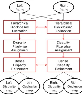
Our symmetric framework combines in a first phase a classical hierarchical block-based method9 (to deal with large disparity range) and recursive filtering-based regularization. A second phase consists in deriving dense disparity maps. In a third phase, an iterative refinement loop classifies pixels as consistent, inconsistent or occluded and refines the two depth maps in the inconsistent areas and finally fills the occlusion areas. In our case, LRC is rather used to force disparity consistency via filtering, and occlusion is detected via another technique, OCC (occlusion constraint10): a disparity map of one view is used to detect the occlusion areas in the other view. Occlusion holes are then simply filled with the nearest background disparity value on the same scanline.

Our symmetric stereo algorithm is illustrated in Figure 2. It provides a dense disparity map with ¼ pixel accuracy and an occlusion map for each view. The three phases are described in the next subsections:

1. Hierarchical block-based estimation 2. Disparity pixel-wise assignment 3. Dense disparity refinement

Figure 2 – Double dense disparity and occlusion estimator

2.2 Hierarchical block-based estimation

2.2.1 Hierarchical block matching (HBM) and filtering

This estimation phase relies on an iterative coarse to fine algorithm that operates on an image pyramid where disparity at a coarser level is used to constrain a more local search at a finer level. Aggregated matching cost is based on normalized cross-correlation computed on luminance signal.

Joint bilateral filtering is introduced at each of the four levels of the HBM estimator, before transmission of the

current disparity map to the next finer level for the three first levels. It is applied to the disparity map in order to smooth it in particular in the textureless areas. The filtering encourages the blocks with similar luminance to have similar disparity. The spatial filter is defined as:

Hierarchical Block-based Estimation Disparity Pixel wise Assignment Dense Disparity Refinement Hierarchical Block-based Estimation Disparity Pixel wise Assignment Dense Disparity Refinement Left frame Right frame Left Disparity map Left Occlusion map Right Disparity map Right Occlusion map

y xy y xy W y d W x dˆ( ) ( ) (1)

where x is the current block, d(u) is the disparity value at block u, y is a block of the NxN blocks window centered on x (N=11). Wxy is the weight assigned to the disparity value of block y. Wxy is defined as follows:

2 1 2 1 xy xy

e

W

xy results from the luminance difference between block x and its neighboring blocks y; it is defined as:

)

(

)

(

y

I

x

I

As the disparity is defined on a block, luminance IB used here corresponds to the average of the luminance data on

the block. xy is defined as the distance in the image grid between block x and block y:

2

y

x

xy (Euclidean norm) (4)

and γ are constant parameters. It is applied at each level with 2 iterations.

Finally, the filtered disparity value dF is selected unless its matching cost is higher than the cost before filtering plus

a penalizing weight , i.e.:

)

(

,

)

(

,

d

x

C

x

d

x

x

C

Consistency constraint is applied at the finest level on the block-based representation. It is introduced via a second bilateral filtering that combines both left and right disparity maps. The filter is given by (dL and dR are left and right

disparity vectors): y xy y xy R L y xy L L

W

x

d

y

d

W

y

d

W

x

d

ˆ

(

)

(

)

(

)

2.3 Disparity pixel-wise assignment and filtering

2.3.1 Disparity assignment

Disparity pixel-wise assignment follows the block-based estimator in order to define a dense disparity map. For each pixel, the current disparity value plus the four values corresponding to the 4-connected neighboring blocks are candidates. The final disparity assigned to pixel x is the one among the five candidates that provides the minimal cost. For each disparity candidate, the color-weighted cost aggregation is performed as follows:

y xy y xy

w

x

d

y

D

w

x

d

x

C

,

,

where x is the current pixel, d() is disparity, y is a pixel of the NxN window centered on x (N=3). The disparity-compensated difference D(y,d(x)) of pixel y with disparity value d(x) is defined as follows:

b g r c J c K c

y

I

y

d

x

I

x

d

y

D

,

where K and J are the left and right images. wxy is the weight of pixel y defined as follows:

xy

e

w

1

(9)

Φxy results from the color difference between pixel x and its neighboring pixels y; it is defined as: b g r c c c xy

I

y

I

x

)

(

)

(

2.3.2 Disparity filtering

Joint trilateral filtering is applied to the dense pixel-wise disparity map in order to decrease noise introduced by the

previous step and increase smoothness in particular in the textureless areas. The spatial filter is defined by:

y xy y xy V y d V x dˆ( ) ( ) (11)

where x is the current pixel, d(u) is the disparity value at pixel u, y is a pixel of the NxN window centered on x (N=21 in our experiments). Vxy is the weight assigned to the disparity value of pixel y. It is defined as follows:

2 1 2 1 2 1 y xy xy D xy

e

V

Γxy and Φxy have been previously defined (Equations (4) and (10)). Dy is the disparity-compensated difference of Equation (8) computed for pixel y with disparity value d(y): Dy =D(y,d(y)). , and are fixed parameters.

The trilateral filtering is combined with median filtering and the set is iterated a fixed number of times.

2.4 Dense disparity refinement

2.4.1 Introduction

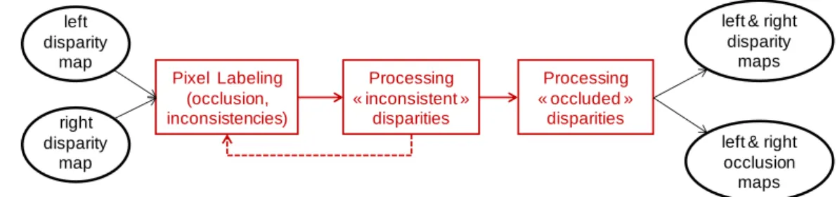
Figure 3 depicts the third phase which objective is mainly to jointly process inconsistencies and occlusions.

Figure 3 – mixed left-right disparity refinement

A first pixel labeling step is the detection in each view of successively: pixels that are occluded in the other view

pixels with an inconsistent disparity vector

pixels which vector points at outside the frame in the other view

The second step consists in jointly filtering both left and right inconsistent disparity maps. These two steps (labeling and filtering) are embedded in an iterative loop.

Once the disparity map has been stabilized, disparity is filled in the “occlusion” areas (third step).

2.4.2 Pixel labeling

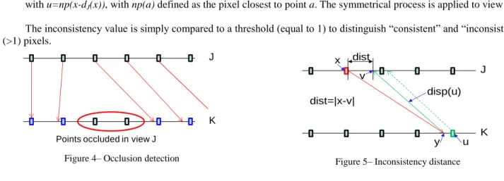
The simple test used to detect occlusions is illustrated in Figure 4 (“OCC” in reference10 ). The pixels in view K that are occluded in view J are detected as follows: considering the disparity map of view J and starting from each pixel in J, its corresponding point in view K is identified via its assigned disparity vector. Then the closest pixel to this point in view K is marked as “visible”. At the end of this visibility detection, the pixels that are not marked are classified as “occluded” in the other view.

Disparity inconsistency is measured via the comparison of the disparity vector in the current view and its corresponding disparity vector in the other view. This is similar to left/right checking (LRC) in reference10 except that this is not used here to detect occlusions. Practically, according to Figure 5, for a given pixel x in view J, its

Pixel Labeling (occlusion, inconsistencies) Processing « inconsistent » disparities Processing « occluded » disparities

left & right disparity

maps

left & right occlusion maps left disparity map right disparity map

inconsistency value corresponds to the sum of the disparity vector dJ(x) of x and of the disparity vector dK(u) of the pixel

u in view K that is the closest pixel to the endpoint of dJ(x) in K with abscissa x-dJ(x):

x

d

x

np

d

x

d

J

x

dist

(

,

)

with u=np(x-dJ(x)), with np(a) defined as the pixel closest to point a. The symmetrical process is applied to view K. The inconsistency value is simply compared to a threshold (equal to 1) to distinguish “consistent” and “inconsistent” (>1) pixels.

Figure 4– Occlusion detection _{Figure 5– Inconsistency distance}

2.4.3 Inconsistent disparity processing

Joint trilateral filtering combining both left and right disparity maps is then applied in the inconsistent areas in

order to force consistency. The weight is defined as in section 2.3.2.

y xy y xy R L y xy L L

V

x

d

y

d

V

y

d

V

x

d

)

(

)

(

)

(

ˆ

2.4.4 Disparity filling in “occlusion” areas

Disparity vectors previously estimated in the occlusion areas (occluded in the other view) are discarded as they are not reliable. These areas are then filled from neighboring disparity vectors visible in both views. Each set of consecutive occlusion pixels along each scan line is processed separately. It is supposed to have an occluding region on one side and a relative background on the other side. So, considering the two corresponding disparity values, each occlusion pixel is replaced by the disparity value that corresponds to the largest depth except if its current value corresponds to a larger distance.

The disparity vectors are finally 2D filtered via bilateral filtering (Equation (11)) where Vxy (Equation (12)) is

limited to Φxy and Γxy, and then median filtering.

2.5 Output

The output is for each pair left and right disparity maps and occlusion maps. Figure 6 shows disparity and occlusion maps of a left view selected in the MPEG 3D “Amelia Retro” sequence (courtesy of DOLBY). Performance evaluation is discussed together with view synthesis in section 4.

Figure 6 – “Amelia Retro” stereo HD sequence (courtesy of DOLBY): left image n°104, corresponding disparity and occlusion maps (dark areas are classified as “occluded in the right view”)

J

K

Points occluded in view J

x y dist=|x-v| u v dist J K disp(u)

3. VIEW SYNTHESIS

The heart of view interpolation consists in interpolating a disparity map for the new view, and then in synthesizing the view by interpolating video information using this interpolated disparity map and the left and right views.

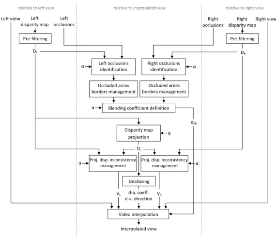
Our view interpolation relies on disparity maps, as can be seen in Figure 7; only the video interpolation in itself uses the original views.

relative to left view relative to interpolated view relative to right view

Left view Pre-filtering Left disparity map Right view Pre-filtering Right disparity map DL DR Right occlusions identification Left occlusions identification α α

Blending coefficient definition Occluded areas borders management Occluded areas borders management Disparity map projection α DI Proj. disp. inconsistency

management αLR VL VR α Video interpolation Interpolated view

Proj. disp. inconsistency management α α Dealiasing d-a. coeff. d-a. direction Left occlusions Right occlusions

Figure 7 - view synthesis overview

3.1 Disparity map projection

In our case the disparity map interpolation consists in projecting the left estimated disparity map onto the view to be synthesized. Our approach is similar to Scharstein’s work11 except that we project only one disparity map.

The position of the view to be synthesized (between the original left and right views) can be defined by a factor, which is applied to the original disparity values. So that if the new view is positioned at alpha times the distance between the left and right views, the disparity values are multiplied by alpha.

The left disparity map is scanned from left to right (so that information concerning occluding pixels overwrites, i.e. occludes, information concerning occluded pixels) and each disparity value is projected (shifted) at the position defined by this scaled disparity. This position is rounded to the nearest pixel location in the projected disparity map.

During this process, because of disocclusion some pixels in the view to be synthesized get no disparity value projected to them. These pixels correspond to objects visible in the synthesized view but occluded in the left view. In order to fill these disoccluded areas, during the projection each disparity value is assigned to all pixels on the right side of the previously assigned pixel up to the pixel the current disparity value points at (Filling with background disparity). The same problem can also occur when two neighbor disparity values close to each other (in value) are projected to two non neighbor pixels in the interpolated view; and the same solution is applied.

3.2 Disparity map pre-filtering

View interpolation relies on disparity maps. Unfortunately the 1-layer disparity map format we use does not allow representing the scene as correctly as the video does. The video pixels can for example render transparency, blur (motion blur, defocus…) or object borders by combining video information of several objects into a single video pixel.

Assigning a disparity to such mixed pixels is a problem since they correspond to two pixels in the other view. In the context of unique correspondence, disparity of such pixels should correspond either to the foreground object or to the background object. However intermediate disparity values may occur during disparity estimation (e.g. due to bilateral filtering); in other contexts such values can be created by anti-aliasing filtering. Such values can lead to artifacts during interpolation and need therefore to be corrected.

The solution consists in identifying narrow disparity gradients and altering the inner disparity values toward outer disparity values.

3.3 Occlusion area identification

Some objects, because of occlusions, are visible in the synthesized view but occluded in the left view or in the right view. To render these parts, only one view will be used.

During disparity estimation, the occlusion areas in the left and right views are identified (section 2.4.2). Therefore in order to identify in the synthesized view regions that are occluded in the left view or in the right view, this informatio n is projected at the new view position.

3.4 Occluded area border management

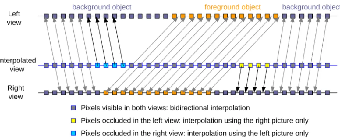
After these operations, we know for each pixel of the new view which view (left or right or both or none of them) can be used (the case where none of them can be used is addressed in section 3.5). During the video interpolation, in the occluded areas only one view will be used to synthesize the new view (unidirectional interpolation), while in the rest of the picture a mix of both views is used (bidirectional interpolation). (Figure 8)

Left view Right view Interpolated view

Pixels visible in both views: bidirectional interpolation

Pixels occluded in the left view: interpolation using the right picture only Pixels occluded in the right view: interpolation using the left picture only

background object foreground object background object

Figure 8 - Interpolation scheme without border management

The transition between these unidirectional (in the disoccluded area) and bidirectional interpolations can however be visible for various reasons. For instance, the disparity map does not necessarily match perfectly the object borders (particularly in case of blurred borders: where is the object border?); this can generate echoes in the new view. Also differences of luminance, color, reflections or flare between left and right views can create halos around objects.

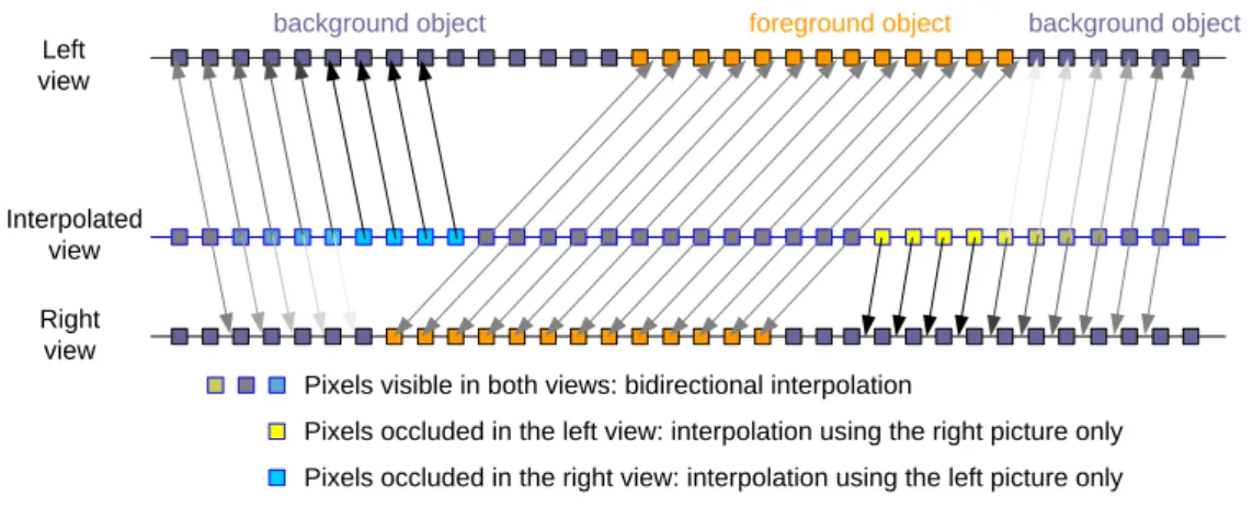
The occluded area borders management aims at reducing the visibility of the aforementioned artifacts. This consists in softening the transition between the unidirectional and the bidirectional interpolations on the border of occluded areas. The coefficients used for the bidirectional interpolation are changed on the right of the regions occluded in the left view, and on the left of the regions occluded in the right view. (Figure 9)

Left view Right view Interpolated view

Pixels visible in both views: bidirectional interpolation

Pixels occluded in the left view: interpolation using the right picture only Pixels occluded in the right view: interpolation using the left picture only

background object foreground object background object

Figure 9 - Interpolation scheme with border management

The blending coefficient definition block assigns a value to the blending coefficient (αLR) depending on the results

of the occluded area borders management, resolving issues of areas located just between regions occluded in the left view and regions occluded in the right view, and also the case of regions occluded in both views.

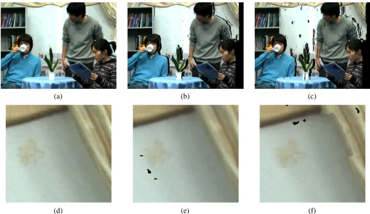
Figure 10 - Results on “Amelia Retro”: (a-c) without border management; (d-f) with border management

3.5 Projected disparity inconsistency management

This blending coefficient (αLR) will be used for the video interpolation to weight the bidirectional interpolation.

However the left or right samples used for the interpolation can possibly not correspond to the correct object. This is for example what happens in regions occluded in both views; the disparity value can have been correctly estimated (i.e. the disparity corresponds to the correct depth of the occluded object), but the disparity value points at foreground objects.

These mismatches between the projected disparity values in the new view and the disparity values they point at in the original views are checked and corrected. This consists in comparing the projected disparity values in the new view with the disparity values of the pixels they point at in the original views. In case of inconsistency, instead of using the pixel the disparity value points at, another pixel will be looked for in the original view; for example the nearest pixel having the corresponding disparity value can be used instead.

This pixel corresponds to an object at the same depth as the supposed occluded object. However it is not sure that this video value correctly represents the occluded object. Also the proposed method will often lead to use a same video value for several neighbor pixels. Therefore more sophisticated solutions, using region filling techniques for example, can be advantageously used. (The proposed solution has the advantage of being simple and in most cases effective since the occluded areas are often small and locally homogeneous.)

After this operation, the two pixels that will be used for the bidirectional interpolation will not necessarily correspond to a same point of the 3D scene. This means that the vectors pointing at these pixels are not necessarily a function of the disparity value (in both directions). Therefore after this consistency operation a disparity value is no longer sufficient to refer to corresponding pixels in the left and the right views, and so vectors (VL and VR) pointed at the

corresponding pixels in each view are used instead.

(f) (e) (d) (c) (b) (a)

3.6 Video interpolation

The new view can then be synthesized. This step consists in interpolating the video values of the new view using the left and right video sources. The video samples used for the interpolation are those pointed by the vectors VL and VR

(we use linear interpolation to point at sub-pixel position). These left and right samples are combined using the blending coefficient αLR.

3.7 Dealiasing

Optionally a dealiasing block can be added. This aims at suppressing the aliasing effect, which can appear on the object borders. This effect occurs because in the 1-layer disparity map format we use, only one disparity value is stored per pixel (cf. section 3.2). Therefore in the disparity map object borders are located at pixel borders. This means that in the interpolated disparity map object borders exhibit aliasing.

Figure 11 - Disparity map and corresponding interpolated video without dealiasing

Our solution consists in using locally a 2-layer representation. But instead of using the video to define an alpha value (using a matting information estimation like in the most common solutions12,13,14), we propose to simply fill the stairs along the object borders with foreground information. This is done by detecting the aliased borders in the interpolated disparity map (by comparing the disparity values) and by virtually adding a sub-pixel shape to smooth these contours. Therefore one line of pixels along the object borders will use two disparity values, and thus a combination of background and foreground information. The piece of foreground video information is interpolated using the blending coefficient and the vectors VL and VR of one of the neighbor pixels (in the direction of the aliased contour) and is then

combined with the not-dealiased sample (background information) using the dealiasing coefficient.

Figure 12 - Disparity map and corresponding interpolated video with dealiasing

The figures 11 and 12 illustrate this process on a basic example. The Figure 11 shows on the left an interpolated disparity map and on the right the result of interpolation without dealiasing. The Figure 12 shows on the left the same disparity map with the virtual shape (of foreground information) to be added onto the background of the aliased contour and on the right the corresponding result with dealiasing. The results on Figure 13 show how the aliasing and the “cut-out” appearance are reduced.

Figure 13 - Results on “Amelia Retro”: (a-c) without dealiasing; (d-f) with dealiasing

(f) (e) (d) (c) (b) (a)

4. EXPERIMENTAL RESULTS AND DISCUSSION

Two sets of experiments have been carried out on MPEG sequences in order to compare our method with available MPEG software16 (VSRS Revision 2216). In both cases, the two methods are compared by assessing resulting synthesized views through our new objective image quality assessment metric VSQA15 (View Synthesis Quality Assessment).

VSQA15 is dedicated to artifacts detection in synthesized view-points. It aims to handle areas where either disparity estimation or interpolation fail by using three visibility maps which characterize complexity in terms of textures, diversity of gradient orientations and presence of high contrast. The quality assessment is done by comparing original and interpolated images with VSQA. For each frame it returns the number of pixels considered by VSQA as erroneous (also called VSQA score). The less this score is, the better the tested approach is.

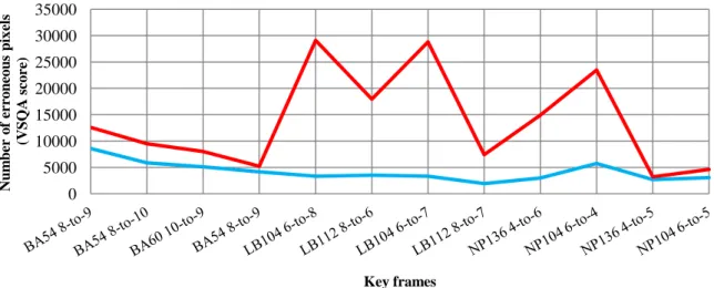
The first experimental test consists in comparing our disparity-compensated view synthesis and the MPEG software in an extrapolation scenario17 (see example Figure 15). Only one camera and the associated depth map are used to render the synthesized views (therefore, occlusions remain). Moreover, the quality assessment is done only for pixels that are considered as visible in the two reference views by the two methods. Test frames from 3 (1024 768) sequences have been used: Book Arrival, Lovebird1 and Newspaper. Figure 16 shows the quality results.

(a) (b) (c)

(d) (e) (f)

Figure 14 – Comparison between the proposed disparity-compensated view synthesis and MPEG disparity estimation and view synthesis. Camera 6 is extrapolated from camera 4 (Newspaper, 136). Original view (a) and zoom on details (d), synthesized view with detected occlusions (proposed approach) (b) and zoom on details (e), synthesized view with detected occlusions (MPEG software) (c) and zoom on details (f).

In Figure 15, we notice that geometric distortions in (c) and (f) are more noticeable in comparison with (b) and (e). More generally, Figure 16 shows that our approach gives synthesized views with a better quality compared to MPEG approach. As previously, the same tests have been performed with the Structural SIMilarity (SSIM) index20 and lead to the same conclusions. All these results prove that our approach exceeds the MPEG disparity estimation and view synthesis in rendering areas visible in both reference views.

Figure 15 - Quality assessment with VSQA metric between extrapolated and original (at the same position) views from Book Arrival (BA), Lovebird1 (LB) and Newspaper (NP) sequences. The extrapolated views are obtained with the proposed disparity-compensated view synthesis and MPEG disparity estimation and view synthesis. Occluded areas are not taken into account.

In a second set of experiments, the disparity estimation and view synthesis modules have been separated and the four possible combinations between MPEG modules and ours have been compared along the whole Book Arrival sequence. This test consists in rendering camera 8 from cameras 10 and 6. The quality assessment is done by comparing original and virtual cameras 8 with VSQA. The main difference with the first experiment is that now the occlusion areas are considered.

Figure 16 - Quality assessment between original and synthesized Book Arrival sequences with VSQA metric. All possible combinations between the disparity estimation and view synthesis modules of the proposed method and MPEG method16 are tested. Camera 8 is rendered from cameras 10 and 6.

Firstly, let us compare blue and purple curves (our disparity estimation with our view synthesis and with MPEG view synthesis respectively) and green and red curves (MPEG disparity estimation with our view synthesis and with MPEG view synthesis respectively) in Figure 14. They show that the same quality level is reached by the two

0 5000 10000 15000 20000 25000 30000 35000 Nu m b er o f er ro n eo u s p ix els (V S Q A sc o re ) Key frames

Our disparity estimation and view synthesis MPEG disparity estimation and view synthesis

0 5000 10000 15000 20000 25000 30000 35000 40000 1 4 7 10 13 16 19 22 25 28 31 34 37 40 43 46 49 52 55 58 61 64 67 70 73 76 79 82 85 88 91 94 97 100 Nu m b er o f er ro n eo u s p ix els (V S Q A sc o re ) Frames

Our disparity estimation and view synthesis MPEG disparity estimation and view synthesis MPEG disparity estimation + our view synthesis Our disparity estimation + MPEG view synthesis

interpolation algorithms. Secondly, if we compare blue and green curves (our view synthesis with our disparity estimation and with MPEG disparity estimation respectively) and purple and red curves (MPEG view synthesis with our disparity estimation and with MPEG disparity estimation respectively), we notice that MPEG disparity estimation gives better results. It is due to the use of 3 original views in the MPEG software for disparity estimation whereas our approach only uses a pair. Consequently, the occluded areas are better rendered with MPEG algorithms. Note that SSIM20 has also been used as quality metric and gives the same conclusions.

A large set of HD real and animation stereo sequences have been processed in order to evaluate our method. Very good results have been obtained in animation sequences. Of course the results are not always as good in real sequences: The worst encountered problems include large occlusions with hardly predictable content (e.g. light visible in one view only), transparency, very thin objects with large disparity range. Between these two extremities, there is space for improving reasonable artifacts either by improving the method itself or developing alternative methods, either with more specific methods adapted to particular complex cases or with masking techniques as a fallback mode.

The quality assessment proposed in our framework can be useful in order to identify the more distorted frames within a sequence. A quality threshold can be set with respect to the required quality level (depending on the application). Only the frames with a VSQA score under this threshold need to be corrected (in a semi-automatic or automatic way).

5. CONCLUSION AND FUTURE WORK

A disparity estimation and view synthesis method has been developed for s3D content correction. Our experiments have shown that the algorithm provides satisfying results in a wide set of stereo data. While we consider that results can be improved in some specific situations via moderate modifications (e.g. occlusions, thin objects), some other cases cannot be satisfactorily processed by our current method (e.g. transparency) and require complex solutions. Large occlusions are also a problem in particular when an object with a particular disparity is present in only one view. These cases where our current method fails are detected via quality evaluation and either automatic or semi-automatic additional tools will be addressed in the future to post-process these failing areas. One promising solution is to consider temporally distant information to solve local ambiguity (e.g. in large occlusions19)

REFERENCES

[1] Devernay, F., Duchêne, S. and Ramos-Peon, A., “Adapting stereoscopic movies to the viewing conditions using depth-preserving and artifact-free novel view synthesis”, Proc. SPIE 7863, paper 1 (2011).

[2] Scharstein, D. and Szeliski R., “A taxonomy and evaluation of dense two-frame stereo correspondence algorithms”, IJCV, 47, 7-42 (2002).

[3] Sun, J., Li, Y., Kang, S., B. and Shum H.-Y., “Symmetric stereo matching for occlusion handling”, Proc. IEEE CVPR, 2, 399-406 (2005).

[4] Zitnick, C., L. and Kanade, T., “A cooperative algorithm for stereo matching and occlusion detection”, PAMI, 22(7), 675–684 (2000).

[5] Yang, Q., Wang, L., Yang, R., Stewénius, H. and Nistér D., “Stereo matching with color-weighted correlation, hierarchical belief propagation and occlusion handling”, IEEE Trans. on PAMI, 31 ( 3), 492-504 (2009).

[6] Xiao, J., Cheng, H., Sawhney, H., Rao, C. and Isnardi, M., “Bilateral filtering-based optical flow estimation with occlusion detection”, Proc. ECCV, 3951, 211-224 (2006).

[7] Boughorbel, F., “Adaptive filters for depth from stereo and occlusion detection”, Proc SPIE 6803, paper 17, (2008).

[8] Paris, S., Kornprobst, P., Tumblin, J. and Durand, F., “A gentle introduction to bilateral filtering and its applications,” in ACM SIGGRAPH Courses, (2007).

[9] Tzovaras, D., Strintzis, M., G. and Sahinoglou, H., “Evaluation of Multiresolution Block Matching Techniques for Motion and Disparity Estimation”, Signal Processing: Image Communication, 6 (1), 59-67 (1994).

[10] Egnal, G. and Wildes, R., “Detecting binocular half-occlusions: empirical comparisons of five approaches”, IEEE Trans. on PAMI, 24(8), 1127–1133 (2002).

[11] Scharstein, D., “Stereo vision for view synthesis”, Proc. IEEE CVPR, 852–858 (1996)

[12] Zitnick, C., L., Kang, S., Uyttendaele, M., Winder, S. and Szeliski, R., “High-quality video view interpolation using a layered representation”, ACM SIGGRAPH, 600–608 (2004).

[13] Hasinoff, S., W., Kang, S., B. and Szeliski, R., “Boundary matting for view synthesis”, CVIU, 103 (1), 22–32 (2006).

[14] Xiong, W. and Jia, J., “Stereo matching on objects with fractional boundary”, Proc IEEE CVPR, 1-8 (2007). [15] Conze, P.H., Robert, P. and Morin L: “Objective view synthesis quality assessment”, Proc. SPIE 8288, Paper 56 (2012).

[16] MPEG, “Report on Experimental Framework for 3D Video Coding”, ISO/IEC, JTC1/SC29/WG11/n11631, (2010). [17] Bosc, E., Pépion, R., Le Callet, P., Köppel, M., Ndjiki-Nya, P., Pressigout, M., and Morin, L., “Towards a new quality metric for 3D synthesized view assessment”, IEEE Journal on Selected Topics in Signal Processing, 5 (7), 1332-1343 (2011).

[18] Mueller, M., Zilly, F. and Kauff, P., “Adaptive cross-trilateral depth map filtering”, Proc. 3DTV conference, (2010). [19] Ndjiki-Nya, P.; Köppel, M.; Doshkov, D.; Lakshman, H.; Merkle, P.; Mueller, K.; Wiegand, T.,“ Depth image based rendering with advanced texture synthesis”, IEEE Trans. on MULTIMEDIA, 13(3), 453-465 (2011)

[20] Wang, Z., Bovik, A., Sheikh, H., and Simoncelli, E., “Image quality assessment: From error visibility to structural similarity”, IEEE Trans. on Image Processing, 13(4), 600-612 (2004).