Correcting the effect of magnetic tongues on the tilt angle of bipolar active regions

HAL Id: hal-02474185

https://hal.sorbonne-universite.fr/hal-02474185

Submitted on 11 Feb 2020

HAL is a multi-disciplinary open access

archive for the deposit and dissemination of

sci-entific research documents, whether they are

pub-lished or not. The documents may come from

teaching and research institutions in France or

abroad, or from public or private research centers.

L’archive ouverte pluridisciplinaire HAL, est

destinée au dépôt et à la diffusion de documents

scientifiques de niveau recherche, publiés ou non,

émanant des établissements d’enseignement et de

recherche français ou étrangers, des laboratoires

publics ou privés.

Correcting the effect of magnetic tongues on the tilt

angle of bipolar active regions

M. Poisson, M. López Fuentes, C. Mandrini, P. Demoulin, C. Maccormack

To cite this version:

M. Poisson, M. López Fuentes, C. Mandrini, P. Demoulin, C. Maccormack. Correcting the effect of

magnetic tongues on the tilt angle of bipolar active regions. Astronomy and Astrophysics - A&A,

EDP Sciences, 2020, 633, pp.A151. �10.1051/0004-6361/201936924�. �hal-02474185�

Correcting the effect of magnetic tongues on the tilt angle of

bipolar active regions

M. Poisson

, M.C. López Fuentes

, C.H. Mandrini

, P. Démoulin

and C. MacCormack

1 _{Instituto de Astronomía y Física del Espacio, IAFE, CONICET-UBA, CC. 67, Suc. 28, 1428 Buenos Aires, Argentina, e-mail:}

mpoisson@iafe.uba.ar, lopezf@iafe.uba.ar

2_{LESIA, Observatoire de Paris, Université PSL, CNRS, Sorbonne Université, Univ. Paris Diderot, Sorbonne Paris Cité, 5 place Jules}

Janssen, 92195 Meudon, France, e-mail: Pascal.Demoulin@obspm.fr

3 _{Universidad de Buenos Aires, Facultad de Ciencias Exactas y Naturales, 1428 Buenos Aires, Argentina, e-mail:}

mandrini@iafe.uba.ar

February 10, 2020

ABSTRACT

Context. The magnetic polarities of bipolar active regions (ARs) exhibit elongations in line-of-sight magnetograms during their emergence. These elongations are referred to as magnetic tongues and attributed to the presence of twist in the emerging magnetic flux-ropes (FRs) that form ARs.

Aims.The presence of magnetic tongues affects the measurement of any AR characteristic that depends on its magnetic flux distri-bution. The AR tilt-angle is one of them. We aim to develop a method to isolate and remove the flux associated with the tongues to determine the AR tilt-angle with as much precision as possible.

Methods.As a first approach, we used a simple emergence model of a FR. This allowed us to develop and test our aim based on a method to remove the effects of magnetic tongues. Then, using the experience gained from the analysis of the model, we applied our method to photospheric observations of bipolar ARs that show clear magnetic tongues.

Results.Using the developed procedure on the FR model, we can reduce the deviation in the tilt estimation by more than 60%. Next we illustrate the performance of the method with four examples of bipolar ARs selected for their large magnetic tongues. The new method efficiently removes the spurious rotation of the bipole. This correction is mostly independent of the method input parameters and significant since it is larger than all the estimated tilt errors.

Conclusions.We have developed a method to isolate the magnetic flux associated with the FR core during the emergence of bipolar ARs. This allows us to compute the AR tilt-angle and its evolution as precisely as possible. We suggest that the high dispersion observed in the determination of AR tilt-angles in studies that massively compute them from line-of sight magnetograms can be partly due to the existence of magnetic tongues whose presence is not sufficiently acknowledged.

Key words. Physical data and processes: magnetic fields, Sun: photosphere, Sun: magnetic fields

1. Introduction

A dynamo mechanism located at the bottom of the convection zone (CZ) is frequently invoked to explain the formation of ac-tive regions (ARs, see e.g. the reviews of Charbonneau 2014; Brun & Browning 2017, and references therein). In this con-text, the magnetic flux is amplified and deformed by di fferen-tial rotation and convective motions until it becomes buoyant and emerges in the form of twisted flux-tubes or flux ropes (FRs). Several magnetohydrodynamic (MHD) simulations of flux emergence consider the rise of coherent FRs from deep in the CZ that will later form ARs, once the rope succeeds to tra-verse the photosphere (see the reviews by Fan 2009; Cheung & Isobe 2014; Toriumi 2014, and references therein). However, there are also numerical simulations that explain the formation of ARs due to the in situ amplification and structuring of the mag-netic field by convection (see the review in Brandenburg 2018)

The structure of the emerging FRs determines the observed characteristics of ARs in line-of-sight (LOS) magnetograms.

Send offprint requests to: M. Poisson

One of these characteristics is the presence of magnetic tongues (López Fuentes et al. 2000), which have been also called tails (Archontis & Hood 2010). If we assume that ARs are formed by the emergence ofΩ-shaped FRs, magnetic tongues are pro-duced by the projection of the azimuthal component along the LOS and they appear in bipolar ARs as elongations of the main polarities with a yin-yang pattern. López Fuentes et al. (2000) reported their existence for the first time in a rotating bipolar AR and they were later observed in many other examples (see e.g. Luoni et al. 2011; Mandrini et al. 2014; Valori et al. 2015; Yard-ley et al. 2016; Vemareddy & Démoulin 2017; Dacie et al. 2018; López Fuentes et al. 2018). They also have been found in nu-merical simulations of emerging FRs (Archontis & Hood 2010; Cheung et al. 2010; MacTaggart 2011; Jouve et al. 2013; Rempel & Cheung 2014; Takasao et al. 2015).

In Poisson et al. (2015a) we presented a systematic method to quantify the influence of magnetic tongues using the evolution of the photospheric inversion line (PIL) during the emergence of bipolar ARs. We measure the acute angle between the estimated PIL and the line orthogonal to the AR bipole axis. From this angle, which we called the tongue angle [τ], we estimated the

average twist present in the sub-photospheric emerging FR under the assumption that it can be modelled using a uniformly twisted half torus. We found that, in general, the twist is below one turn. In a subsequent article (Poisson et al. 2015b), for a set of sim-ple bipolar ARs, we compared the twist computed as in Poisson et al. (2015a) with the twist inferred using a linear force-free field model of the AR coronal field. The signs of the twist esti-mated from both methods are consistent. Furthermore, we found a linear relation between the twist derived from the analysis of tongues and that obtained from the coronal field model.

In Poisson et al. (2016), we studied how the tongues af-fect the evolution of the magnetic flux distribution of ARs. This study was done for bipolar ARs observed over more than one solar cycle. We also developed a more sophisticated FR emergence model that considered loop cross-sections with non-uniform twists (both in the radial and azimuthal directions). We found that the effect of tongues tends to be stronger at the be-ginning of the evolution and weaker as the AR emerges. We also found a variety of evolutions that suggested, by comparison with the model, that emerging ARs have a wide set of twist profiles.

Although the results obtained by Poisson et al. (2016) pro-vide constraints to theoretical and numerical models of FR emer-gence, they do not provide a method for removing the effects of the tongues from the intrinsic characteristics of emerging FRs. One of these intrinsic properties is the inclination of the emerg-ing FR with respect to the solar equator, usually defined as the tilt angle. The distribution of tilt with solar latitude sets constraints on dynamo models. In addition, there has been an important ef-fort over the past few years to characterise the tilt of ARs with a diverse range of results (Li & Ulrich 2012; McClintock & Nor-ton 2013; McClintock et al. 2014; Wang et al. 2015; Tlatova et al. 2018). As we demonstrated in Poisson et al. (2015a, 2016), the presence of tongues has a non-negligible effect on the determina-tion of the tilt. We consider that part of the disperse (also taking into account the sometimes inconsistent results found by obser-vational studies determining the tilt of ARs) can be affected by the lack of consideration for the effect of magnetic tongues in the measurements.

In this work, we introduce a method to compute the intrinsic tilt-angle of bipolar ARs using LOS magnetograms. The method aims to remove the effect of the magnetic tongues when comput-ing the barycentres of the polarities and, hence, to obtain the AR tilt angle that better represents the intrinsic tilt. This method is defined in Sect. 2 following a summary of the the analytical FR model used to test it. In Sect. 3, we explore the parameter spaces of the model and of the method to evaluate the tilt correction and analyse the strengths and weaknesses of the method. Next, in Sect. 4, we describe the four bipolar ARs used in Sect. 5 to evaluate the method. These selected emerging ARs have strong magnetic tongues, which implies a strong deviation of the AR tilt deduced directly from the magnetograms. Finally, in Sect. 6, we summarise and discuss our results.

2. Flux rope model and the tilt correction method

In this section, we first summarise the main characteristics of the FR model defined in Luoni et al. (2011), then extended in Poisson et al. (2016), in order to set a framework to test the new method designed to remove the effect of magnetic tongues on the tilt of ARs.

(a)

(b)

(c)

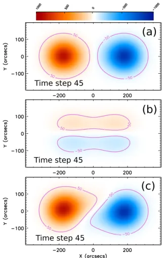
Fig. 1. Synthetic magnetograms of the axial (a) and the azimuthal (b) magnetic field components of a uniformly twisted torus model with Nt,0= 0.5. (c) Total superposed magnetic field map. The red- and

blue-shaded areas represent the positive and the negative value of Bz. The

magenta contour in each map corresponds to |Bz| = 50 G (the

maxi-mum axial field is set to 1000 G). The associated movies are available online (fig1_a.avi, fig1_b.avi, and fig1_c.avi).

2.1. The simple flux emergence model

The simple FR model, developed in Luoni et al. (2011), provides a global description of the evolution of the photospheric mag-netic field during the emergence of bipolar ARs. It consists of a toroidal FR with uniform twist (both along and across its axis). The sign and amount of magnetic twist is given by imposing a number of turns [Nt] to the magnetic field lines. Ntcorresponds

to half of the emerging torus (see Figure 2 in Luoni et al. 2011). The axial field component is supposed to have a Gaussian profile in the FR cross section (a distribution typically present in numer-ical simulation of FRs in the CZ). The upper half of the torus is set to progressively emerge without distortion. Therefore, this simple model does not take into account the deformations and reconnections occurring during emergence.

The emergence of the FR at the photospheric level provides a series of synthetic magnetograms, which are analysed in exactly the same way as observed magnetograms (Sect. 5). The proce-dure consists in cutting the toroidal rope by successive horizon-tal planes (z = constant, where z is vertical coordinate), which play the role of the photosphere at successive times, and com-puting the magnetic field projection in the direction normal to these planes [Bz]. These synthetic magnetograms are the result

Time step Tilt angle [deg]

Nt,0 = 0 (0,0) Nt,0 = 0.2 (0,0) Nt,0 = 0.5 (0,0) Nt,0 = 0.7 (0,0) Nt,0 = 0.5 (1,0) Nt,0 = 0.5 (-1,0) Nt,0 = 0.5 (0,0.8) Nt,0 = 0.5 (0,-0.8) Time step 10 Time step 45

(c)

(a)

(b)

Fig. 2. (a)-(b) Synthetic magnetograms for the FR emergence model with Nt,0= 0.5 (h = 0, g = 0) at two different time steps of the evolution. The

red and blue dashed-contours correspond to the |Bz|= 50 G isocontours of the axial field map (Fig. 1a). The magnetic field strength on the FR axis

is set to 1000 G. The red and blue dots show the position of the magnetic barycentres of the axial map and the black segment in between indicates an intrinsic tilt φi= 0. The |Bz|= 50 G isocontours of the total map (see also Fig. 1c) are drawn with magenta continuous lines. The magenta line

that joins the total map barycentres indicates an apparent tilt φa. (c) Evolution of φafor the uniform-twist models with Nt,0= 0, 0.2, 0.5, 0.7 (black,

red, green and blue continuous lines, respectively). The non-uniform twist models have a fixed value of Nt,0 = 0.5 and (h, g) values indicated

between brackets (violet, yellow, orange, and brown continuous lines, respectively). The associated movie is available online (fig2_a.avi).

of the torus (Bφand Bθ, respectively) projected in the z-direction (see an example in Figure 1 of Poisson et al. 2015b). Henceforth, each cut, that is, each magnetogram, is identified with a time step number in an analogous way to the observation time of ARs. For all the models that we use in this work, we set the number of cuts at 65.

In order to identify the effect of tongues on the synthetic magnetograms, in Fig. 1a–b we separate the axial and azimuthal field components for time step 45. The axial field component map (Fig. 1a) has a mirror symmetry with respect to the y-direction which corresponds to the PIL y-direction. In this exam-ple, the FR is oriented in the x-direction and the tilt is null. When we add the azimuthal component map (Fig. 1b), we obtain a magnetogram in which the polarities are elongated producing magnetic tongues (Fig. 1c). This change is caused by the com-bination of two effects. In the top part of the positive polarity (y > 0), both the azimuthal and axial field components con-tribute to a positive Bz, thus enhancing it compared to the

no-tongue case. In the bottom part of the positive polarity (y < 0), the azimuthal component contributes to a negative Bz and thus

partially cancels the positive Bz-signal from the axial

compo-nent. The reverse occurs in the negative polarity, with the en-hancement of the negative polarity occurring in the bottom part (y < 0) and the cancellation in the top (y > 0) part. Both en-hancement and cancellation of the field components, result in an asymmetric shape of each polarity, so in the presence of mag-netic tongues.

In Poisson et al. (2016), the aforementioned simple model was extended to interpret the evolution of the PIL and tilt angle in ARs with a large variety of twist profiles. For half of a torus-shaped FR with a major radius [R], a minor radius [a], and a field strength on the axis [B0], we define the azimuthal field in

the natural coordinates of the torus {ρ, φ, θ} as

Bθ(ρ, θ)= 2 ρ Nt(ρ) B0e−(ρ/a)

2

/(R + ρ cos θ) , (1) where ρ is the distance to the torus axis, φ is the angle describ-ing the position along the torus axis, and θ is the rotation angle around this axis. The modifications we introduced include a non-uniform twist profile [Nt(ρ)] along the radial direction of the FR

cross-section that depends on a single non-dimensional parame-ter, called h. We define the non-uniform twist profile as

Nt(ρ)= Nt,0max(1+ h (ρ/a)2, 0) . (2)

For h = 0, the FR is uniformly twisted as the model presented in Luoni et al. (2011). A value of h > 0 implies a twist more concentrated at the edge of the FR; as an example, if h = 1 the twist at ρ= a duplicates the value at the centre. Similarly, h < 0 implies a twist decreasing from the axis to the FR border.

We introduce a simple θ-dependence on the torus axial field, which produces a non-uniformity of the twist in the azimuthal direction:

Bφ(ρ, θ) = B0asy(θ) e−(ρ/a)

2

,

with asy(θ) = (1 + g cos θ) , (3)

where g is the parameter controlling the non-axisymmetric level of Bφ. This parameter introduces a strong asymmetry between the top and the bottom parts of the FR cross-section. If g > 0, the twist is lower in the top part of the FR cross-section than in its bottom part and, conversely, if g < 0. Both parameters, h and g, vary within the interval [-1, 1] and strongly affect the evolution of the magnetic tongues (see Appendix B in Poisson et al. 2016). Figure 2a-b shows two time steps in the FR emergence when Nt,0 = 0.5 and h = g = 0 (i.e. they correspond to the uniformly

twisted FR). The intrinsic tilt angle [φi] of this FR is φi = 0; it

is indicated with a black continuous line joining the barycentres of the axial field as the FR emerges. When the torus is cross-ing the photospheric plane in the first steps, the projection of the azimuthal field in the normal direction increases. As a conse-quence, the flux of the tongues becomes stronger and shifts the position of the barycentres towards the elongated region of each polarity, producing a spurious increase of the tilt angle, that is, an apparent tilt angle [φa]. The magenta dots show the position

of the barycentres computed from Bzand the solid magenta line

marks the tilt direction obtained from these barycentres. Fig. 2c illustrates the evolution of the tilt angle for the torus model with different values of Nt,0 and (h, g). In this panel, the green line

corresponds to the model shown in the left panel. We conclude that the deviation of φafrom φicould be significant.

2.2. Core Field Fit Estimator

The separation of the axial and the azimuthal field components from only a Bzmagnetogram is an ill-posed problem. Since we

cannot identify both components separately, we define the core and the tongue regions as the areas on the magnetogram that best represent the extension of the axial and azimuthal compo-nents, respectively, and we develop a method to approximately locate and constrain each of these regions on synthetic Bz

mag-netograms.

The procedure aims to locate on each synthetic magnetogram the magnetic flux in the FR core region, which is the closest to the axial flux. Henceforth, we refer to this method as the core field fit estimator (CoFFE). The segment between the centres of the core flux region of each polarity is the one we use to estimate the FR tilt-angle [φc]. One of the main advantages of using our

FR model (Sect. 2.1) to design this method is that we can test our procedure by comparing φito φc, which, in the best scenario,

should be the same.

We approximate the core field distribution assuming that it is symmetric with respect to the core centre position and with a decreasing profile towards the borders. We use a Gaussian function for our procedure because that is the profile of the ax-ial field distribution in the simple FR model. An axisymmetric Gaussian function has five free parameters: the maximum field strength [Bmax], the magnetic baseline level [B0], the position of

the Gaussian centre [xmax, ymax], and the mean dispersion around

the centre, or simply the half width [σ]. We fix B0= 0, since the

mean background field is null in our synthetic magnetograms. The Gaussian function is fitted using an IDL routine based on the non-linear least-squares fitter MPFIT. Since the effect of the azimuthal field component in emerging ARs typically decreases with time, as it is the case in the model, we first apply the fit to the last magnetogram of the series. For the FR model, when the half torus is fully emerged, that is, at magnetogram 65, the Gaus-sian fit is exact due to the absence of the azimuthal component and the Gaussian distribution selected for the axial component. Next we use the parameters of the fit at step i as an initial guess to estimate the Gaussian for the magnetogram at step i − 1. This way of proceeding improves the stability of the method, assum-ing that consecutive magnetograms have similar magnetic flux distributions.

We now present how we proceeded and applied our method. Figure 3a shows the magnetogram for the model with uniform twist (Nt,0 = 0.5) at time step 32, which is when the LOS

pro-jection of the azimuthal flux is maximum (Fig. 4a). The black circles correspond to the contour levels drawn at half the max-imum of the Gaussian function fitted over each polarity. This

fitting has been done using the information of the entire magne-togram. In this first step, we identify areas where the magnetic flux departs from the Gaussian distribution. We represent those areas with green and blue isocontours for the flux that is larger and lower by a given amount than the fitted Gaussian, respec-tively. We fix this amount to 50% of the maximum difference between the Gaussian function values and the synthetic magne-togram. These contours are labeled in Fig. 3a on the positive polarity (symmetric contours are present on the negative polar-ity). The largest of these isocontours (labeled 1 and 2) repre-sent the asymmetry generated by the presence of the azimuthal field. The outer isocontours (3 and 4) are produced by the shift of the position of the Gaussian peak towards the tongues. These last isocontours should be very small; they should not even be present at all when we have a good approximation to the core field distribution.

We use the information obtained from the first fitting (Fig. 3a), which we call zero iteration, and redo the fit by mask-ing those points where the asymmetry is the largest, that is, where the excess or lack of flux with respect to the Gaussian function is larger. To do this we select a region between the Gaussian centres as the one delimited by the red lines in Fig. 3b and c. The red lines are defined with a linear function which crosses the core centre of the respective polarity and it is also orthogonal to the bipole axis defined by φcin the previous

iter-ation. The region defined between these lines is used to exclude those points from the map at the next iteration, that is, Fig. 3b, which is obtained excluding a region that was defined at iteration zero but the lines shown in this panel enclose the region that is to be excluded in the next iteration. In this way, we consider the flux of the polarities with less contribution from the azimuthal field. The removal of the points is done using a weighting op-tion; we assign a weight of 1 or 0 to the points that are outside or inside the limited region, respectively. We call this new compu-tation (see Fig. 3b) as the first iteration of the method. Once we get the new parameters of the Gaussian, a new limited region for the next iteration is defined (see Fig. 3c).

We repeat this procedure until we consider we have found the best fit to the core field distribution. We set lower and upper limits to the number of iterations [nit] we carry out for each

mag-netogram. We fix the lower limit to four iterations. We chose to stop the computation when φcvaries by less than 1◦between two

successive iterations. We call Citthe minimum iteration in which

this convergence criterion is fulfilled. In summary, the method automatically iterates Cittimes at time step i and then uses the

fitted parameters as a first guess for the parameters at time step i −1.

Figure 3c corresponds to the Gaussian fitting for nit = 4.

One of the outer isocontours (4 in Fig. 3a) has vanished but the other one is still present. Although the latter contour is smaller than in the first iteration (Fig. 3b), the remaining flux below the Gaussian means that the points removed at each iteration are not enough to fully eliminate the effect of the tongues from the com-puted tilt angle. Therefore, we modify the region that is excluded using a single parameter p that shifts away from the polarity cen-tres each of the red lines by a quantity p σ where σ is the width of the fitted Gaussian. If p is positive, the region is to be ex-tended. Figure 3d shows the same magnetogram of panel c but with the Gaussian computed with p = 1. The main difference between these two panels is in the size and location of the green and blue isocontours. Removing a larger area of the polarities means that we reduce the effect of the tongues when we fit the core field. In Fig. 3d, the increase of the green contours corre-sponds better to the location of the tongue flux. We can increase

1 2 3 4

(a)

(b)

(c)

(d)

Time step 32

Fig. 3. (a) Synthetic Bzmagnetogram for the torus model with uniform twist (Nt,0 = 0.5, h = 0, g = 0) at time step i = 32. We use the same

coloured code and isocontours levels for Bzthan the ones used in Fig. 1. The black circles over each polarity represent the contour level of 0.5Bmax

of the Gaussian function that best fits the magnetic field distribution. The position of the maximum value for each Gaussian is marked with a+ symbol. The green and blue isocontours indicate the areas where the field is larger and lower than the fitted Gaussian, respectively (by 50% of the maximum difference between the Gaussian function values and the synthetic magnetogram). The red lines, defined as discussed in Sect. 2.2, delimit the area which is excluded from the computation of the Gaussian fit in the next iteration step. (b) Same as (a) but one iteration step forward in the procedure (nit= 1). (c) Three iterations further (nit= Cit= 4). The associated movie is available online (fig3_c.avi). (d) Same as (c) but with

the exclusion area extended one σ (Gaussian width) towards the outer part of the magnetic bipole (see Sect. 2.2).

even more the exclusion region but at some point the amount of flux removed from the computation affects the goodness of the fit and the stability of the iterative procedure.

The standard error on the position of the Gaussian centre, xmaxand ymax, can be computed using the diagonal elements of

the covariance matrix obtained with the non linear least-square fit. But these errors are too small and do not reflect the goodness of the model to approximate the polarity core field. In particu-lar, the effect of the exclusion region is not well accounted for considering only the standard deviation of the fitting parameters. Therefore, we consider another type of error, more intrinsic to the CoFFE method. We compute φcusing values of p within

the interval [−1, 1] to delimit the range of the tilt angle correc-tion. We consider p= 1 as an upper limit due to its impact on the fitting procedure. For p > 1 the exclusion region removes more than 85% of the core flux significantly degrading the goodness of the fit. Conversely, for p < −1, more core flux is added to the fit but the tongue flux included also increases as p becomes more negative.

3. Correction of the tilt angle for a FR model

In this section, we apply the CoFFE method (described in Sect. 2.2) to isolate the core flux along the emergence of the modelled FR described in Sect. 2.1. We scan different twist pro-files and we investigate how the results depend on the parameters of the CoFFE method.

3.1. First tests

The evolution of the total magnetic flux [Fz] of each AR

po-larity in the model with Nt,0 = 0.5 is shown in Fig. 4a (black

line). The green and blue lines correspond, respectively, to the evolution of the FR axial and azimuthal flux contributions in the synthetic magnetograms. The difference between the black and green curves changes during the emergence. This difference cor-responds to the effect of the tongues on Fz. The tongue effect

peaks when the FR is about halfway emerged.

Even though the effect of the tongues becomes smaller as we go closer to the end of the emergence, the field enhancement pro-duced by the tongues is enough to modify the maximum of Fz.

This maximum is reached before the half torus is fully emerged (see black-dashed vertical line in Fig. 4a) at step 57, while the effect of the azimuthal flux disappears at step 65 when the half the torus has emerged. We henceforth call this effect Bz

enhance-ment. This implies that at the time of maximum flux we can still have strong magnetic tongues and, therefore, the time of maxi-mum flux cannot be used to identify the end of the emergence (even if it seems to be a logical choice).

3.2. Convergence tests

The corrected tilt angle [φc] is determined by the acute

an-gle between the x−axis and the line that joints the core cen-tres with the CoFFE method, meaning its tongue effects have been removed, while the apparent tilt φais the tilt deduced from

the full magnetogram using the barycentres. Figure 4b shows the computed φa and φc using the model with uniform twist

nit = 0 & p = 0 nit = Cit & p = 0 Φa Φc: p=1 p=-1 Time step Model Nt,0 = 0.5 (0,0)

(a)

(b)

Tilt angle [deg]

p=0

Fig. 4. (a) Evolution of the magnetic flux computed from the synthetic magnetograms for the FR model with uniform twist (Nt,0= 0.5, h = g =

0) during its emergence. We plot the magnetic flux [Fz] (black line), the

axial flux [Faxial

z ] (green line), and the azimuthal flux [Fazimuthalz ] (blue

line). All fluxes are computed for the z component of the fields. All fluxes are normalised to the maximum axial FR flux. (b) Evolution of the apparent tilt φa computed from the magnetic barycentres (on the

full magnetogram, black line) and φcusing CoFFE with p= 0 for two

nitvalues (see the inset). The coloured-shaded area surrounding the red

line represents the φcrange obtained for different values of p within

the interval [−1, 1] after the convergence criterion of the tilt angle is achieved.

(Nt,0 = 0.5, h = 0, g = 0). The green and red lines show the

evolution of φc obtained by CoFFE with p = 0 and for nit =

0 and Cit, respectively. They correspond to the Bz distributions

shown in Fig. 3a,c. φcbecomes closer to φi = 0 as the number

of iterations increases, which shows that the method converges well.

To estimate an error for the tilt angle derived from the CoFFE method, we compute φcfor different values of p. For each model,

we compute nine estimations of φc for equispaced values of p

within the interval [−1, 1]. These values are displayed in Fig. 4b with a red-shaded area. As p is more negative the tilt is closer to the result obtained at the zero iteration (green curve). As it is expected the inclusion of more flux of the tongues (p more neg-ative) produces a smaller shift of the Gaussian centres towards the core so less tilt correction. In contrast, a larger positive p value increases the Gaussian centre displacement at each iter-ation achieving a more significant correction of the tilt angle. Despite the broader range of φcobtained from time step 15 to 0,

two aspects are noteworthy. First, the results with p > 0 (above

the red curve with p= 0) are closer to φialong most of the FR

emergence. More specifically, we find that for p = 1 the varia-tion of φcreduces to 8◦away from φi= 0, compared to the

vari-ation of ≈ 20◦for φa(black line). This implies a decrease of the

tongue effect by ≈ 60% when using the extended region p = 1. Secondly, the mean value of Citcomputed along the emergence

ranges between the minimum iteration number (4) and a mean of 5.15 for all the different values of p; this means that the method has a fast convergence to a stable value of φcat each time step.

3.3. Effects of the twist amplitude

Next we selected different Nt,0values to test how the strength of

the azimuthal field affects the stability of our method and the cor-rection of the tilt angle. Figure 5 shows the magnetic flux and φc

evolutions for models with low and high uniform twist. In panel (a) we show the evolution of the magnetic flux (continuous lines) and the azimuthal flux (dashed lines) for both models, Nt,0= 0.2

in black and Nt,0 = 0.7 in red. The maximum azimuthal flux

in the first case is around 10 % of the total axial magnetic flux. Therefore, there is no significant Bzenhancement and the total

maximum flux is reached at the end of the emergence at time step 65 (black line). On the contrary, the model with Nt,0 = 0.7 has

a large enhancement of Bzthat causes the shift of the maximum

flux to time step 50 (red vertical line).

In Fig. 5b–c we show the evolution of the apparent tilt φa

for models with Nt,0 = 0.2 and Nt,0 = 0.7 (black lines). Despite

the reduced effect of the azimuthal flux for the case with Nt,0=

0.2, there is a 10◦_{variation of the apparent tilt angle during the}

emergence that departs from the FR intrinsic tilt, φi= 0. The tilt

variation for the Nt,0 = 0.7 model is around 30◦, that is ≈ 10◦

larger than the model with Nt,0= 0.5 (Fig. 4b).

Next we use CoFFE with nit = Cit, implying that

conver-gence is achieved, to compute a corrected tilt angle. The red lines in Fig. 5b–c show the evolution of φccomputed with p= 0 with

Nt,0 = 0.2 and Nt,0 = 0.7, respectively. Using p = 0 we reduce

the difference between the corrected tilt φc and φi in

approx-imately 45% of the original difference derived from φa (black

line). The percentage of correction is nearly independent of the FR twist strength (see Figs. 4 and 5). The best correction of φc

for both models is obtained with p= 1 (φccloser to 0). For the

Nt,0 = 0.2 model, φcdeparts from the intrinsic tilt in less than

4◦along the full FR emergence and even below 2◦between time steps 20 to 50. For Nt,0= 0.7 the correction reduces the apparent

rotation of the bipole to a 12◦counter-clockwise rotation for the case p= 1. More generally, in all the models shown we are able to reduce the difference between φcand the intrinsic tilt of the

bipole by about 60% along the FR emergence.

With even higher p values, that is of 1.5 and 2 (not shown here), and despite the large amount of flux removed from the fitting procedure, we are above an 80% correction in all cases, reducing the difference between φcand φibelow 10◦along the

full FR emergence for the model with Nt,0 = 0.7. However, the

amount of flux removed from the procedure with these values of pabove 90 % of the core flux makes the fit unstable, especially in real ARs where the core field does not follow in general a Gaussian profile.

The FR model used has no deformation of its main axis (the FR axis is located in a plane). However, from the evolution of the apparent tilt φawe find a spurious rotation of the polarities

produced by the magnetic tongues that can be wrongly related to the FR writhe, which corresponds to the deformation of the FR axis as a whole (López Fuentes et al. 2000). All models with positive twist have an apparent rotation in a counter-clockwise

(c)

(a)

(b)

Tilt angle [deg]

Tilt angle [deg]

Time step p=1 p=-1p=0 p=1 p=-1 p=0

Fig. 5. Comparison of the magnetic flux and the tilt angle evolution for uniform twist models (h= 0 and g = 0) with Nt,0= 0.2 and Nt,0= 0.7.

(a) Evolution of the magnetic flux, Fz(continuous lines), the azimuthal

flux, Fazimuthal

z (dashed lines), and the axial flux, Faxialz (green-continuous

line) for the models with Nt,0 = 0.2 (black) and Nt,0 = 0.7 (red). The

vertical continuous lines (with the same black and red colours) show respectively the time step in which each model reaches its maximum Fzflux. The black-dashed vertical line indicates the time step in which

Fazimuthal

z is maximum. All fluxes are normalised to the maximum Faxialz .

(b)-(c) Evolution of the tilt angle for models with (b) Nt,0= 0.2 and (c)

Nt,0= 0.7. The black and red lines show the tilt angle estimations of φa

and φc(see inset), respectively. The red-shaded areas correspond to the

values of φccomputed for p within the interval [−1, 1]. The associated

movies are available online (fig5_b.avi and fig5_c.avi).

sense due to the tongue retraction, suggesting a torus geometry with a positive writhe. Several studies have estimated the writhe of ARs from the evolution of the tilt angle along their

emer-gence (López Fuentes et al. 2003; Liu et al. 2014; Yang et al. 2009). Our analysis suggests that the magnetic tongues have a strong impact on the correct estimation of the tilt in agreement with López Fuentes et al. (2000), who first show that the retrac-tion of magnetic tongues could induced a fake rotaretrac-tion of an AR bipole, even reversing its direction of rotation during emergence. The correction achieved with CoFFE reduces this spurious rota-tion significantly, providing a more reliable estimarota-tion of the FR writhe.

3.4. Non-uniform twist

Next we study the model with non-uniform twist using the h parameter as a measure of the radial profile of the twist (see Sect. 2.1). We keep Nt,0 = 0.5 and we change h using its

ex-treme value of 1 as reference. Figure 6a shows the Bz map at

different time steps for the model with h = 1 which corresponds to a flux-rope with an enhanced number of turns of 1 at the pe-riphery of the torus (in comparison to Fig. 3). This increase of the azimuthal field is reflected in the strong elongation displayed by the tongues during all the emergence of the FR. In Fig. 6b the azimuthal flux (blue line) is larger than the axial flux (green line) till the first third of the emergence. The strong enhancement of the azimuthal magnetic flux shifts the maximum flux (black dot-ted line) to time step 43, far from the end of the FR emergence. In this case, the location of the maximum Fzis closer to the

maxi-mum azimuthal flux, which indicates that the tongues are strong at this time. This fact supports the statement mentioned above that the maximum flux is not a good reference to establish the centre location of the core field. At this time step the LOS pro-jection of the azimuthal field masks most of the characteristic features of the axial field distribution.

Figure 6c shows that the apparent tilt angle, φa(black line),

has a large variation of 60◦ due to the long and persistent mag-netic tongues. φc, derived from CoFFE with p = 0 (red line),

partially corrects the tilt angle achieving a variable correction ranging from 25% at the first third of the emergence phase and up to 50% towards the end of the emergence. Comparatively, the estimation for p= 1 (red-shaded area upper boundary) produces a more stable computation of φcand provides about 55%

correc-tion of φccompared to φaalong the FR emergence.

This test case with h = 1 represents an extreme instance where the azimuthal flux is larger than the axial flux during the first third of the emergence. The few ARs interpreted as formed by highly twisted FR develop other signatures on their flux distri-bution, apart from the magnetic tongues, that can be linked to the writhe of the main axis of the FR. In those cases, the magnetic tongues are difficult to interpret due to the development of kink instabilities that produce complex ARs with non simple bipolar magnetic field distribution (López Fuentes et al. 2003; Poisson et al. 2013; Dalmasse et al. 2013).

Next, the models with negative h and positive g have signifi-cantly reduced tongues (see Fig. A.1a-b in Appendix A), so the effect of the magnetic tongues tongues is comparable or lower than the already studies case with Nt,0= 0.2.

Finally, a negative g parameter produces a strong variation of the apparent tilt φaalong the FR emergence (see Fig. A.1c

in Appendix A). Despite the large variation of φa, this case has

results similar to the case with strong magnetic tongues using the h= 1 model (Fig. 6).

Time step Tilt angle [deg]

Model Nt,0 = 0.5 (1,0)

(b)

(a)

(c)

Fig. 6. (a) Synthetic Bzmagnetograms for the model with a twist profile increasing with the radial coordinate of the torus (Nt,0 = 0.5 and h = 1,

defined in Eq. (2) at time steps 4, 19, 34, and 49). We use the same colour code and contours as in Fig. 3. The segments join the polarities barycentres (magenta line) and the core centres (black line). (b) Computed Fz(black), Fzazimuthal(blue), and Faxialz (green) along the FR emergence.

Dashed-vertical lines indicate the time step of each maximum flux with their respective colour. All fluxes are normalised to the maximum value

of Faxial

z . (c) Evolution of the apparent tilt φacomputed from the magnetic barycentres (black line) and of φcusing CoFFE (see the inset). The

red-shaded area corresponds to the values of φccomputed for p within the interval [−1, 1] after the convergence criterion of the tilt angle is achieved.

The associated movie is available online (fig6_a.avi).

4. Data Used

We applied CoFFE to LOS magnetograms of ARs obtained with the Michelson Doppler Imager (MDI: Scherrer et al. 1995) on board the Solar and Heliospheric Observatory (SOHO). The full-disc magnetograms with 96-minute cadence are obtained by averaging either one-minute and five-minute magnetograms. The different averages results in a flux density errors of 16 G and 9 G per pixel, respectively. These data provide 15 magnetograms per day with a size of 1024 × 1024 pixels and a spatial resolution of 1.9800_.

We use the same temporal and morphological criteria to se-lect ARs as described in Poisson et al. (2015a). The sample con-sists of ARs with a low background flux, whose emergence phase is observed during their transit across the solar disc. We limit the latitude and the longitude of the emergence to ± 30◦ _{from the}

solar equator or the central meridian (CM), respectively. This criterion aims to minimise foreshortening and projection effects when the AR is close to the solar limb (Green et al. 2003). In order to describe the behaviour of our new method on

observa-tions, we select four bipolar ARs; these ARs are representative of regions with strong tongues. This selection is best to test the abil-ity of CoFFE to remove the tilt deviation associated to magnetic tongues. Furthermore, because CoFFE performs better when the tongues are less extended (lower tilt correction), we prefer not to exemplify such cases.

To obtain the set of magnetograms to which we applied CoFFE, we processed the full-disc magnetograms using stan-dard Solar-Software tools. We first transformed the magnetic-flux density measured in the LOS direction to the solar radial direction, neglecting the contribution of the components on the photospheric plane. This is a small correction as the selected ARs are close to the disc centre. The effects of this transforma-tion were analysed by Green et al. (2003). Then we rotated the magnetograms to the date when the AR was located at the CM and we removed from the set any magnetogram with evidence of wrong pixels.

Next we chose rectangular boxes of variable size encom-passing the AR polarities during the emergence phase in order

Tilt angle [deg] Magnetic fl ux [10 22 Mx 2 ] 3000 1500 0 -1500 -3000 10 Aug 2001 11:15 UT

AR 9574

(a)

_(b)

1

2

3

4

(c)

Fig. 7. (a) SOHO/MDI LOS magnetograms of AR 9574. The red- and blue- shaded areas represent the positive and the negative Bzmagnetic field

component. The magenta contour in each map corresponds to the field magnitude of ±50 G. The black circular contours are the half-width level of the Gaussian fit for each polarity using p= 0 and nit= Cit. The green and blue isocontours indicate the areas where the field is larger and lower

than the Gaussian, respectively, by 50% of the maximum difference between the Gaussian and the local observed field. The black and the magenta segments show the tilt of the AR respectively obtained with the core flux centres (which define φc) and the magnetic barycentres (which define the

apparent tilt φa). (b) Evolution of the AR magnetic flux computed from the magnetograms. The vertical dashed line marks its maximum value. (c)

Evolution of φaderived from the magnetic barycentres (black line) and φcobtained with CoFFE (see inset). The red-shaded area corresponds to the

values of φccomputed for p within the interval [−1, 1] after convergence criterion of the tilt angle is achieved. The associated movie is available

online (fig7_a.avi).

to minimise the contribution of the background magnetic flux (Poisson et al. 2016). Movies for each AR were made to verify that the variable size box included all the magnetic flux of the AR at all times. All the AR parameters were computed consid-ering only the pixels inside these rectangular boxes.

5. Correction of the tilt angle for ARs

The application of CoFFE to the models in Sect. 3 has shown that p is the most relevant parameter to obtain the best approx-imation to the intrinsic tilt of the bipole. We have shown that a proper selection of p can improve the computed tilt φceven in

those cases where the azimuthal field is stronger than the axial

field. It is noteworthy however, to see that increasing the p value also increases the uncertainty of the fitted Gaussian parameters (because smaller portions of the magnetograms are used for the fits). In this section, we present the φcresults determined for four

ARs and we test the dependence of the tilt correction on different values of p.

For each of the four selected ARs, we studied diverse condi-tions that help us to test the performance of CoFFE. We started with an AR which has a clear separation between the core and the tongue components, facilitating the core selection made with CoFFE. Then we analysed a more complicated case where the tongues are completely linked to the core distribution, as it hap-pens for the FR model. Increasing the tongue flux complexity,

we studied the tilt correction in an AR where the tongues have a fragmented structure because of the emergence of a secondary bipole located at the centre of the AR. Finally, we tested CoFFE in an AR that has strong tongues all along the analysed time span and a partially observed emergence limited by the longitudinal criterion of Sect. 4.

As we have seen in Sect. 3, we expect the core magnetic flux to be dominant at the end of the FR emergence. However, while for observed ARs we may not be able to see the full emergence, we still use the last magnetogram of the set as the initial refer-ence to start the computation.

Despite the complexity of the observed ARs, magnetic tongues have a field distribution that is typically easy to recog-nise and locate in the LOS magnetograms by simple visual in-spection. Conversely to the models of Sect. 3, where the tongue and core fluxes have a continuous overlap, the tongue flux is typ-ically more separated from the core flux in ARs. In the case of observed ARs no intrinsic tilt is available to test the CoFFE re-sults, then, we qualitatively consider that a fit of the core is good when the field that is above the Gaussian, that is, the green con-tours in Fig. 7a, 8a, 9a, and 10a approximately coincide with the observed magnetic tongues.

It is worth noting that the flux of the core in ARs does not follow in general a Gaussian profile. Furthermore, this core flux profile varies from AR to AR; therefore, without having a clear flux profile for all ARs and in an effort to apply our method uni-formly, we decided to use the profile that is better applied to the modelled FR for observed ARs. On the other hand, a Gaussian profile is the simplest and has the lower number of free param-eters still keeping most of AR core characteristics (i.e. a maxi-mum of the flux and a width).

5.1. Results for AR 9574

AR 9574 emerged between 10 and 13 August 2001. The time span for this AR encompasses 55 magnetograms limited accord-ing to the longitude criterion defined in Sect. 4. This bipolar AR emerged in a low magnetic field environment and close to the equator (S3). Figure 7a shows a set of four MDI magnetograms corresponding to its emergence phase. The red- and blue-shaded areas on the magnetograms represent the strength of the outward and inward components of the radial magnetic field. We refer to this field as Bzas it is equivalent to the field on the synthetic

mag-netograms. The magenta isocontours correspond to |Bz| = 50

G. Elongated polarities associated to strong magnetic tongues are present all along the AR emergence. Despite the asymmetric elongation between the leading and the following polarity, we recognise a magnetic tongue pattern that corresponds to a FR with positive twist.

CoFFE provides the approximate location and extension of the core field on each polarity. The circular black contours in Fig. 7a correspond to 50% of the fitted parameter Bmaxon each

polarity. The location of Bmaxfor each polarity is marked with a

black dot. The core field distribution is obtained using p= 0 and nit = Cit. For these parameters, we obtain the best tracking of

the core field centre back to the first flux emergence of AR 9574 (see “fig7_a.avi” in the supplementary material).

Green and blue contours show the regions where Bzis

signif-icantly above and below the Gaussian values, respectively. The values of those contours are expressed in Gauss over the drawn lines and set on each magnetogram as half the maximum dif-ference between Bzand the fitted Gaussian. The green contours

outline the spatial extension of the magnetic tongues (Sect. 3.1). The blue contours are dominant on the core regions indicating

that the Gaussian profile is not completely correct to approxi-mate the field closer to the core centre. As a consequence of this discrepancy, we notice that the observed field on the centre of the polarity is less concentrated than the Gaussian function de-termined with CoFFE.

CoFFE excludes a region around the central PIL of the AR from the tilt computation (Sect. 2.2). The red lines show the lim-its of the exclusion region in Fig. 7a with p = 0. Finally, we show the lines that join the core field centres (black segment), and the magnetic barycentres of the full magnetogram (magenta segment) to compare φcand φatilts.

The emergence near the central meridian passage allows us to analyse the evolution starting from the first flux emergence, that is, when the AR flux is below 10% of the maximum flux observed. A fast flux emergence rate is present in the first half of the evolution in association to the early development of strong magnetic tongues (Fig. 7b). The last half of the emergence has a lower flux emergence rate similar to what we obtained for dif-ferent models in Sect. 3. The latter evolution corresponds to the progressive reduction of the tongue magnetic flux.

Figure 7c shows the evolution of the tilt angle computed along the emergence of AR 9574. We define a positive tilt angle when the leading polarity is closer to the equator than the fol-lowing one, consistently with the Joy’s law. The method with no iterations (nit = 0) and p = 0 (green line) performs similarly as

the other cases with higher nitand p parameters, except at the

be-ginning of the emergence (see below). This implies that CoFFE removes the tongues in a similar way independently of the pa-rameter values so that the core flux is properly identified. This is the case because the spatial separation between the tongues and the core distributions is more pronounced than for the mod-elled cases in Sect. 3, as seen by comparing Fig. 7a with Fig. 3. Archontis & Hood (2010) described a fragmented configuration of the tongues due to the convergence of vertical plasma flows on the photosphere producing tongue regions where the field is compressed. This produces a discrete structuring of the tongues that makes them more distinguishable than in the FR model.

Both cases, with nit= 0 or nit = Cit, and p = 0 have a

con-sistent and clear evolution along most of the AR emergence, but they cannot track back the core centre when Fzis below about

10% of its maximum. That short time span can only be corrected with CoFFE using nit = Citand the extended region of p = 1

(upper limit of the red-shaded area).

The tilt φcdeparts significantly from the apparent tilt φafor

all the time span of the AR emergence. The difference between φcand φaranges from 5◦up to 25◦(Fig. 7c), which is above the

uncertainties estimated for CoFFE (red-shaded area). We also find that there is an opposite tilt of the bipole determined with CoFFE (φc) and the magnetic barycentres (φa). The mean φais

≈ −2◦_{while the mean for φ}

cis approximately 10◦(for p = 1).

The estimated values of φc correspond to an AR located at the

southern hemisphere accordingly to Joy’s law and indeed AR 9574 is in the southern hemisphere.

Moreover, there is an opposite tendency for the bipole ro-tation determined with φcand φa, suggesting different signs of

FR writhe for each estimation. The rotation computed with φc

is around 15◦_{in the clockwise direction (negative writhe), while}

the evolution of φaindicates a counter-clockwise rotation of 5◦

(positive writhe). In this case the magnetic tongues affect the de-termination of the tilt angle changing both the intrinsic tilt and the rotation direction of the bipole.

2700 1350 0 -1350 -2700 21 Jan 2003 23:59 UT 22 Jan 2003 23:59 UT 23 Jan 2003 23:59 UT 24 Jan 2003 23:59 UT

(a)

1

2

3

4

Tilt angle [deg]

AR 10268

(b)

(c)

Magnetic

fl

ux

[10

Mx

]

Fig. 8. (a) SOHO/MDI magnetograms of AR 10268. The magnetograms have the same contours and colour convention as described in Fig. 7a. (b) Evolution of the AR magnetic flux computed from the magnetograms (black-solid line). The vertical-dashed line marks the time at which the AR 10268 reaches its maximum flux. (c) Evolution of φaderived from the magnetic barycentres and φcobtained with CoFFE (see inset). The drawing

conventions are the same as in Fig. 7. The associated movie is available online (fig8_a.avi).

5.2. Results for AR 10268

Figure 8a shows four magnetograms of the emergence phase of AR 10268, each of them labelled with a number that indicates their temporal order. AR 10268 emerged in the north hemisphere (N12) around midday of 21 January 2003. The 5-day long evo-lution of the AR is only limited by the longitudinal criterion (see Sect. 4), restricting the number of analysed magnetograms to 71. This AR has a clear bipolar configuration and magnetic tongues that are more interwoven with the main core field than in AR 9574. There is a small secondary bipole emerging northward of the leading polarity (magnetograms 3 and 4 in Fig. 8a), but

this has only a weak impact on the apparent tilt φa, as the

mag-netic tongues, with their larger fluxes, are the main cause of the shift of the magnetic barycentres towards the AR centre (see also “fig8_a.avi” in the additional material).

As in AR 9574, AR 10268 has two different flux emergence rates (Fig. 8b). The first part is associated with the fast devel-opment of tongues and the consequent enhancement produced on the observed field Bz. After January 23, around the

mid-emergence phase, there is a decrease in the flux mid-emergence rate. The evolution of the apparent tilt φa(i.e. without tongue

AR 9748

p=1

p=-1

p=0

Tilt angle [deg]

Magnetic

fl

ux

[10

Mx

]

(c)

(b)

(a)

1

2

3

4

Fig. 9. (a) SOHO/MDI magnetograms of AR 9748. The magnetograms have the same contours and colour convention as Fig. 7a. (b) Evolution of the AR magnetic flux computed from the magnetograms (black line). (c) Evolution of φaderived from the magnetic barycentres (black line) and

φcobtained from the core flux centres with the same coloured pattern and input parameters as the ones used in Fig. 7c. The associated movie is

available online (fig9_a.avi).

tilted bipole which opposes to Joy’s law prediction (Fig. 8c). The largest departure from the E-W direction reaches up to −25◦_.

Towards the end of the emergence φa tends to a more regular

tilt value, in agreement with Joy’s law, ≈ 20◦_{. However, a}

dif-ferent tilt evolution is obtained after removing the tongues with CoFFE method as φc≈ 0◦initially and it grows progressively to

φc≈ 20◦(Fig. 8c). For p within [0, 1] we get a consistent

evolu-tion of φcand a large departure from φaduring more than the first

half of the emergence phase. Later on, when the tongues retract (Fig. 8a), φcvalues are consistent with φa(Fig. 8c). The di

ffer-ence between CoFFE and the barycentres estimation ranges from around 25◦to 1◦towards the end of the observed emergence. Fi-nally, the mean number of iterations along the AR emergence is below 6, which implies a fast convergence of the procedure to a stable and consistent φc.

The rotation of AR 10268, derived from φa has a sudden

change during the first half of the emergence (see black line in Fig. 8c). Indeed, φameasurements imply a spurious 20◦

counter-clockwise rotation observed until 23 January and then a large clockwise rotation of ≈ 45◦ _{towards the end of the emergence.}

Using the φc estimation for nit > 0 and p > 0, we are able

to completely remove the initial spurious rotation and we get a consistent clockwise rotation of ≈ 20◦along the full emergence. We achieve a better approximation to the intrinsic rotation of the bipole, which is consistent both with the Joy’s law and with the emergence of a FR with a negative writhe. In this case the signs of the twist and the writhe coincide.

5.3. Results for AR 9748

AR 9748 emerged in the southern hemisphere (S11) and close to the east limb on 21 December 2001. We analyse its five-day long evolution across the solar disc which corresponds to 72 LOS magnetograms. The last magnetogram used corresponds to a longitudinal position close to W30◦, so the evolution is trun-cated before reaching the end of the emergence. Figure 9a shows

AR 9906

Tilt angle [deg]

nit = 0 & p = 0 nit = Cit & p = 0 Φa Φc:

(a)

(b)

(c)

1

2

3

4

Fig. 10. (a) SOHO/MDI magnetograms of AR 9906. The magnetograms have the same contours and colour convention as Fig. 7a. (b) Evolution of the AR magnetic flux computed from the magnetograms (black line). (c) Evolution of the apparent tilt φaderived from the magnetic barycentres

(black line) and φc obtained from the core flux centres with the same coloured-pattern and input parameters as the ones used in Fig. 7c. The

associated movie is available online (fig10_a.avi).

four magnetograms illustrating the evolution of AR 9748 mag-netic flux distribution. From the initial stage of the emergence a bipolar distribution is present with a large tilt with respect to the equatorial direction. The elongated magnetic tongues pattern is more complex than in previous examples as it is formed of frag-mented polarities that change of location. For most of the AR evolution we recognise a tongue pattern which indicates that the AR is produced by the emergence of a FR with negative twist (e.g. Fig. 9a on 23 December), while the initial tongue pattern at the beginning of the emergence rather indicates a FR with posi-tive twist (e.g. Fig. 9a on 21 December).

The core fit shown in Fig. 9a was obtained with p= 0 and the number of iterations for convergence (nit = Cit). The magnetic

tongues mostly coincide with the green contours, although they seem to be mixed with other field elements, like a secondary bipole and/or magnetic field remnants present between both core field centres (see “fig9_a.avi” in the additional material). Despite the complex field distribution and strong tongues observed in the

last magnetogram, the method successfully locates the main core field contribution and it effectively tracks it back along the full observed evolution of the AR (Fig. 9c).

AR 9748 has nearly a constant magnetic flux emergence rate along most of the observed evolution. Only near the end there is a small decrease of this rate (Fig. 9b). Comparing this flux evolution with the FR model examples we infer that the stud-ied interval corresponds to about the first half of the emergence phase shown in Figs. 4a and 5a. The time at which the flux emer-gence rate changes coincides with the maximum extension of the magnetic tongues (see “fig9_a.avi” in the additional material).

Figure 9c shows the tilt φa computed from the magnetic

barycentres (black line) and the estimations of φcwith the same

set of parameters as in the previous AR example. For p in [0, 1], we obtain similar results while there is a clear difference between φaand φcthat ranges between 4◦and 7◦and is larger than the

es-timated uncertainties. As seen in all the previous examples, the method performs efficiently requiring a low number of iterations

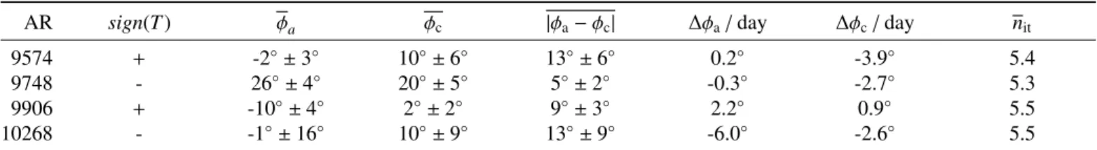
Table 1. List of the analysed ARs and their computed parameters using the magnetic barycentres and CoFFE. Column one and two show the AR NOAA number and the twist sign [sign(T )] derived from the magnetic tongues. Columns three to seven list the values of the mean φaand φc, the

mean difference between both tilt estimations [|φa−φc|], and the variation of the tilt angle [∆φa] and [∆φc] per day; all these values are expressed

in degrees. Finally, the right column shows the mean number of iterations [nit] required for the computations. The errors reported in columns three

to five correspond to the standard deviation of the temporal averages. The values correspond to p= 0.

AR sign(T ) φ_a φc |φa−φc| ∆φa/ day ∆φc/ day nit

9574 + -2◦± 3◦ 10◦± 6◦ 13◦± 6◦ 0.2◦ -3.9◦ 5.4

9748 - 26◦± 4◦ 20◦± 5◦ 5◦± 2◦ -0.3◦ -2.7◦ 5.3

9906 + -10◦± 4◦ 2◦± 2◦ 9◦± 3◦ 2.2◦ 0.9◦ 5.5

10268 - -1◦± 16◦ 10◦± 9◦ 13◦± 9◦ -6.0◦ -2.6◦ 5.5

to achieve a stable φcvalue. The mean number of iterations along

the AR emergence is below 5.5 in the cases where p = 0 and p= 1.

φameasurements imply a strong apparent counter-clockwise

rotation of the polarities of around 14◦_{due to the presence of the}

magnetic tongues, which can be observed along the first day of the emergence. This rotation is removed when we compute φc

and instead we find a constant clockwise rotation of the bipole of ≈ 13◦ (Fig. 9c). The inversion of the rotation sense observed with φaduring the first analysed day of AR 9748 evolution,

can-not be explained as the emergence of a single coherent FR. This kind of change would imply an unrealistic scenario where the FR have mixed writhe along its main axis. The results achieved with CoFFE are consistent with a single emerging FR.

5.4. Results for AR 9906

Finally, we tested CoFFE with the partial emergence of AR 9906. During its solar disc transit, AR 9906 (S16) presented strong magnetic tongues with a pattern associated to a FR with positive twist. In this case, we were able to study only part of the emergence as we could not include the initial flux emergence and the maximum flux was reached far beyond the limit imposed by the longitude criterion. The temporal interval covers five days between 12 and 17 April 2002.

Figure 10a shows selected magnetograms of the emergence phase of AR 9906. The full set of 75 magnetograms is shown in the movie “fig10_a.avi”, which is included in the additional material. We find that CoFFE provides a good approximation of the core field distribution for p= 0 and achieving convergence (nit = Cit) at all times studied. Both the Bzfield regions above

and below the fitted Gaussian, defined as in the previous exam-ples, can be well identified by the green and the blue contours, respectively. Despite their small extensions, the blue contours in Fig. 10a (panels 1, 2, and 3) show the regions in which the core field symmetry is affected by the tongue field of the opposite polarity. The locations of these regions are similar to those ob-served for the FR model in Figs. 3 and 6, but as it was mentioned previously with regard to AR 9574, there is a discrepancy be-tween the Gaussian profile used and the field distribution around the core centre. However, the green contours are well delimiting the magnetic tongues. Hence, all the field contributions are well isolated by the method. This example has the field distribution that most resembles the model used in Sect. 3 (see Fig. 6a).

This AR has a slow emergence rate that allows us to have a good temporal resolution of the first half of the emergence. Figure 10b shows that the magnetic flux increases with a con-stant rate. Comparing this case with the other ARs, the magnetic flux evolution suggests that the AR does not reach the time cor-responding to half FR emergence (see Sect. 2.1). Interestingly,

this example shows how CoFFE responds in a case in which the tongues flux is as strong as the core flux at all times.

Figure 10c shows the φa evolution (black line) and the φc

estimations using CoFFE with the same set of parameters and colour convention as for the previous ARs analysis. The di ffer-ence between both tilt angle estimations ranges between 16◦to 5◦, being around 8◦at the last analysed magnetogram. This dif-ference is far above the estimated uncertainties. In this case, the magnetic tongues mostly add a constant shift to the estimated tilt, producing a tilt angle that opposes the Joy’s law prediction. This effect is mostly removed with CoFFE, achieving a better estimation of the FR axis intrinsic tilt at all analysed times. The computed difference between φaand φcis also above the mean

dispersion reported in several Joy’s law studies (e.g. Wang et al. 2015; McClintock & Norton 2016). Similarly to what we have seen in the previous examples, there is a strong apparent rotation of ≈ 11◦ _{in the counter-clockwise sense due to the evolution of}

the magnetic tongues, while CoFFE provides an almost constant tilt along the same period of time.

5.5. Summary of the AR results

In Table 1, we compare the different tilt-angle parameters ob-tained from both estimations, magnetic barycentres, and CoFFE with p= 0, for the analysed ARs. The four ARs were selected as representative bipolar regions showing strong tongues along their full observed emergence. Columns one and two show the AR NOAA number and the twist sign identified from the mag-netic tongues as done by Luoni et al. (2011). In columns three and four we compare the mean tilt angles, apparent and derived from CoFFE, computed along the AR emergence and noted φ_a and φc, respectively. In three cases, ARs 9574, 9906, and 10268,

magnetic tongues affect the field distribution producing values of the apparent tilt φasuch that the sign of φais opposite to Joy’s

law (Figures 7c, 8c and 10c). In contrast, the estimation of φcis

in accordance with Joy’s law along most of the AR emergence. Column five in Table 1 shows the mean difference between both estimations [|φa−φc|]. There is a significant difference

be-tween φaand φc, especially in the aforementioned cases the mean

correction achieved with φcis above 9◦. It is noteworthy that the

largest correction corresponds to AR 10268, a case in which the tongue flux is more entangled to the core, and therefore, repre-sents the most difficult scenario expected for the optimal perfor-mance of CoFFE.

In columns six and seven we show the mean tilt variations per day [∆φa] and [∆φc], respectively. The tilt variation per day

is defined positive (negative) when it corresponds to a counter-clockwise (counter-clockwise) rotation of the bipole. We chose to show these two quantities to highlight the role of magnetic tongues on