Conception of a near-IR spectrometer for ground-based observations of massive stars

Conception of a near-IR spectrometer for ground-based observations

of massive stars

C. Kintziger*

a

, R. Desselle

a

, J. Loicq

a

, G. Rauw

b

, P. Rochus

a

a

Centre Spatial de Liege, Avenue du Pré-Aily, 4030 Angleur, Belgium;

b

Groupe d’Astrophysique

des Hautes Energies, Institut d’Astrophysique et de Géophysique, Université de Liège, Allée du 6

Août, 19c, Bât B5c, 4000 Liège, Belgium

ABSTRACT

In our contribution, we outline the different steps in the design of a fiber-fed spectrographic instrument that intends to observe massive stars. Starting from the derivation of theoretical relationships from the scientific requirements and telescope characteristics, the entire optical design of the spectrograph is presented. Specific optical elements, such as a toroidal lens, are introduced to improve the instrument’s performances. Then, the verification of predicted optical performances is investigated through optical analyses such as resolution checking. Eventually, the star positioning system onto the central fiber core is explained.

Keywords: Spectroscopy, instrumentation, massive stars, TIGRE telescope, optical design.

1. INTRODUCTION

1.1 Astrophysical Background

The full understanding of astrophysical sources requires access to a rather wide wavelength range. Every wavelength domain provides another specific piece of information that is needed to solve the puzzle. However, some wavelength domains have been somewhat neglected in recent years, despite their enormous potential. This is the case for instance of the near-IR domain around 1-1.1 μm, notwithstanding the fact that this wavelength domain can be accessed from the ground. The main reasons for this situation are the decrease in sensitivity of conventional CCD detectors in this region and the fact that most instruments are designed for longer wavelength studies, e.g. to study the J (1.22 μm), H (1.63 μm) and K (2.19 μm) bands which are largely used in photometry.

The near-IR domain around 1 μm has an enormous diagnostic potential for stellar activity and stellar winds. Stellar winds are prominent features of massive stars, i.e. stars at least ten times more massive than our Sun. Indeed, these stars are very hot and luminous. Their strong UV radiation fields drive energetic and dense stellar winds that have a strong impact on the surrounding interstellar medium. In this context, the wavelength domain near 1 µm is particularly interesting as it contains many spectral lines whose profiles provide useful information about stellar winds over almost the entire range of stellar masses. For example, this region contains the He I λ 10830 line, one of the few unblended He I lines. As it forms over almost the entire stellar wind, it has a huge diagnostic potential for models of stellar winds. Its morphology ranges from an absorption line in stars with low density winds to a broad P-Cygni profile in Wolf-Rayet stars1,2. In some cases, the emission part of the P-Cygni profile is flat-topped, in other cases it is rounded or strongly peaked3. Whatever the morphology, it is related to the velocity law in the wind and can thus provide unique information. Moreover, this line is a good indicator of variability in the wind3, especially for the so-called Luminous Blue Variables, which are in an intermediate evolutionary stage between O and Wolf-Rayet stars where important quantities of material are lost.

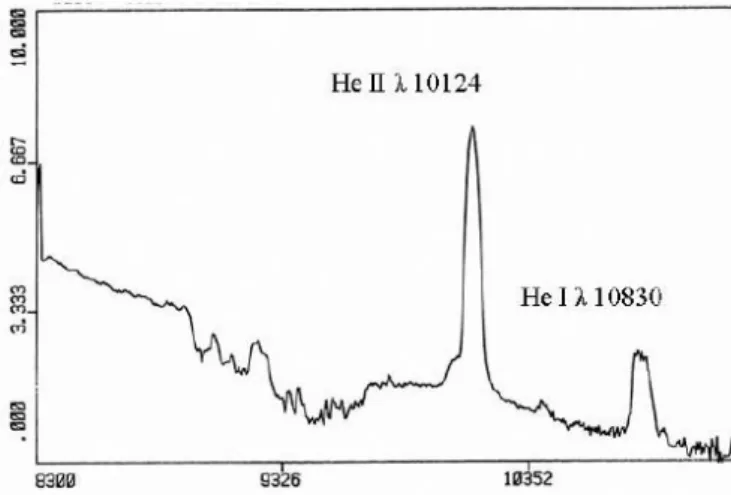
Last but not least, phase-resolved observations of the He I λ 10830 line in massive binary systems are a powerful diagnostic of wind-wind interactions in these binaries4. But He I λ 10830 is of course not the only interesting line in this spectral domain (see Figure 1). Other features include He II λ 10124, Pa δ and Pa γ, C III and C IV lines…

On the other hand, this spectral region is also of interest for studies of the activity of low mass stars. In cool M dwarf stars, chromospheric activity is a wide-spread phenomenon which manifests itself through quiescent line emission (Ca II H & K, Hα) in the optical in addition to dramatic flaring events. Recently, it has been shown that emission in the higher order Paschen lines of hydrogen (Pa β, Pa γ, and Pa δ) as well as He I λ 10830 is a good proxy of a strong flaring activity5,6,7. Also, in the case of solar-type stars, He I λ 10830 and the Paschen lines are excellent indicators of chromospheric activity8.

Moreover, this spectral range provides also key information on the circumstellar environment of cool giants. Indeed, in some cool giants such as Arcturus (K2 III), a highly variable He I λ 10830 emission has been observed and was attributed to shock waves in an otherwise elusive chromosphere9. Yet in other objects such as HD6833 (G9.5 III) the line was found in absorption, but with a bluewards extension that reveals the existence of a stellar wind10.

Finally, the He I λ10830 line is also of major interest for the study of accretion in classical T Tauri stars. T Tauri stars are low-mass pre-main sequence stars that are still accreting material from a circumstellar disk. The emission lines observed in the spectra of these stars form at the star-disk interface or in the inner disk region. These regions have a complex topology. The high opacity of He I λ10830 makes it a sensitive probe of both the accreting matter, in emission, and the outflowing gas via the frequently detected absorption features. Observations of this line in T Tauri stars can thus be used to constrain the wind geometry of such accreting objects11,12.

In summary, it is obvious that the spectral region around the He I λ 10830 line has a huge potential for many topics in stellar astrophysics. Therefore, several research groups from Liège University have joined their forces to develop a spectrograph that covers this wavelength domain with the goal to install it at the TIGRE telescope.

Figure 1. Observation of the near-IR spectrum of the Wolf-Rayet star WR1362 recorded with a CCD detector. The absorption features between 8900 Å and 1 μm are due to the Earth’s atmosphere. (Figure courtesy Jean-Marie Vreux).

1.2 TIGRE

The TIGRE, formerly called Hamburg Robotic Telescope (HRT), is a fully robotic telescope located in La Luz, Mexico13 (see Figure 2). This private telescope is installed at an altitude of 2400 meters on a site operated by the University of Guanajuato. TIGRE is a collaboration between the universities of Hamburg (Germany), Guanajuato (Mexico) and Liège (Belgium).

Currently, the only scientific instrument under operation on the TIGRE is HEROS, a double-channel spectrograph fed with the telescope’s light through an optical fiber. First spectroscopic light in La Luz was achieved in April 2013 and regular automatic observations from Hamburg started on August 1st 2013.

The TIGRE is a F/8 Cassegrain telescope whose primary mirror has a diameter of 1.2 m. The typical seeing at the La Luz site amounts to 2 arcsec on average, approaching 1 arcsec for good nights. Therefore, this telescope is particularly well suited for the study of bright stars. The telescope benefits from a modern Alt-Az mount and concentrates light through a 3-mirror assembly to a Nasmyth focus. The spectrographic instrument that we present will be connected to the telescope through a fiber whose entrance will be placed at the currently vacant Nasmyth focus of the TIGRE telescope. The other end of this fiber will feed with light the instrument located in a separate building neighboring the telescope dome.

Figure 3. The TIGRE telescope at La Luz observatory site, Mexico14.

The characteristics of the TIGRE telescope are summarized in the table below.

Table 1. Characteristics of the TIGRE telescope

Parameter

Symbol

Value

Diameter _Atel 1.2 m

Focal length _ftel 9.6 m

Typical seeing  2 arcsec

1.3 Proposed near-infrared spectrograph

Although those wavelengths can be observed from the ground, the near-infrared region is somewhat neglected due to technological issues such as the decrease in sensitivity of conventional CCD detectors in that spectral domain. We have designed a near-infrared spectrograph to partially fill the gap in this area.

The optical design features a minimum resolution equal to 20 000 within the waveband of interest that ranges from 1 to 1.1 µm. A rotating grating enables the scan of smaller waveband regions to cover the entire wavelength domain. On the other hand, wavelength calibration and flat-fielding are performed with the help of internal calibration lamps that can be selected by a translation stage.

The instrument’s interface consists in a fiber-bundle that feeds the collimator mirror with stellar light from the telescope. On the other hand, a simultaneous sky background measurement is accomplished through the use of dedicated fibers surrounding the central ones, which are located near the target position within the telescope focal plane. Eventually, the circular bundle input is reshaped into a linear configuration to form the entrance slit of the spectrograph.

The fiber option to connect the spectrograph to the telescope opens up the possibility to use the instrument also at other telescopes in the future. A versatile interface was therefore required to enable such capabilities and the choice of using a fiber bundle was made.

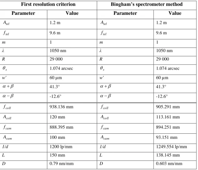
Table 2. Scientific requirements for the proposed near-infrared spectrograph

Parameter

Requirement

Goal

Spectral range 1000-1100 nm 940-1400 nm Resolving power 10 000 20 000 Target magnitudes V < 7 V < 9 Signal-to-noise ratio in continuum 100 at V = 6 100 at V = 7

Typical exposure time 15-30 min 15 min Simultaneous sky measurements yes yes Wavelength calibration accuracy



/200.05Å



/200.025Å

2. OPTICAL DESIGN

2.1 Basic considerations

The scientific requirements impose the spectrograph resolution to be at least 10 000, the ultimate goal being 20 000 over the spectral range 1-1.1 µm. Therefore, each resolved wavelength element has to be ideally equal to:

000 20 R if Å 525 . 0    R mean





In order to discretize each wavelength resolution element with at least two pixels and to cover the waveband of 100 nm, the detector must have a minimum number of pixels equal to

3810 0525 . 0 100 2   pix N

Since typical near-infrared detectors incorporate pixels that are 30 micron wide, a first assessment of the required detector size can be carried out. Indeed, considering a pixel size of 30 µm and the previously calculated number of pixels, the following detector size is obtained:

115 30

*

3810 µm mm

Det_size 

The results show that the required detector size is approximately equal to 12 cm and that the number of pixels exceeds the typical available detector sizes limited to approximately a thousand pixels. The direct consequence is that the total waveband of interest may not be covered in a single exposure unless an echelle spectrograph is considered. In our case, the imaging direction is used for sky background measurements as well as potential other targets falling onto the bundle and therefore, the solution consisting in using a cross-disperser is currently not foreseen.

The reciprocal dispersion or plate factor may also be evaluated in first approximation. This parameter is usually expressed in nm/mm or Å/mm and depicts the variation in wavelength that is measured as the focal plane is swept through. Considering the required wavelength resolution element and the typical pixel size of near-infrared detectors, the reciprocal dispersion is equal to

/ 875 . 0 30 * 2 nm 0.0525 mm nm µm P 

Further calculations involving spectrograph relations must be performed to obtain accurate instrumental requirements. The next section intends to evaluate the required optical elements to achieve the scientific requirements specified in table 2.

2.2 From scientific requirements to technical ones

The first choice before starting any optical design or parameter calculation is to decide upon the nature of the dispersive element used inside the spectrograph, i.e. whether using a diffraction grating or a prism. According to Jacquinot analyses, grating outperform similar size prisms by a factor of 50 to 100 in the near-infrared15 and a grating spectrograph is therefore selected. A Czerny-Turner configuration is adopted from the several ones that exist. One of its advantages is the co-planarity between entrance and exit slits that is enabled through the separation of the collimating and focusing functions of the instrument. On the other hand, more degrees of freedom are made available to the designer thanks to the additional mirror element, which helps to tackle the optical aberrations16. Moreover, the ability to cover a wide spectral range by, for example, rotating the grating makes it a suitable candidate to record the spectrum of the whole required waveband17. Eventually, several studies identified techniques to deal with the inherent aberrations of this design.

When starting the conception of a new instrument from scratch, the first step is to translate the scientific requirements into technical specifications. This means obtaining rough estimates or relations between parameters involved in the optical design of a spectrometer. The complicated side of this problem lies in the fact that several parameters appear when considering a whole spectrograph. Some are given through the scientific requirements but others have to be deduced. The focal lengths of the collimating and focusing optics or the grating spatial frequency are some examples of variables that must be quantified.

Bingham identified sixteen parameters for a grating spectrograph combined to a telescope and proposed a systematic approach to calculate them18. The method concerns plane reflection gratings but can be adapted to curved ones. Those parameters are:

Table 3. Parameters involved in the description of a spectroscopic instrument

Symbol

Parameter

R Resolving power

D Dispersion [mm/nm or mm/Å]

s



Angular entrance slit size





 Sum of incidence and diffraction angles on grating





 Difference between incidence and diffraction angles on grating

m Grating order

tel

A Diameter of the telescope’s primary mirror

tel

f Focal length of telescope

coll

A Collimator size

coll

f Focal length of collimator

cam

A Focuser/camera size

cam

f Focal length of focuser/camera L Grating size (across grooves)

w' Exit slit size

λ Wavelength

Bingham’s method consists in maximizing figures of merit and fixing some basic parameters to obtain all the others in such a way that the derived instrument satisfies the scientific requirements properly. The relations used to derive the entire set of parameters are basic equations describing a standard reflection spectrograph. These are listed below:

d m L L f A D f A w R A R cam cam cam cam tel s















2 cos 2 sin 2 '                  (1)

 

A

 

L Acoll _ cam _





cos cos (2) tel coll tel coll f f A A _ (3)

 

 

tel tel cam cam coll cam f A A f f f M  





cos cos (4)

where M is the magnification of the spectrograph (see R.G. Bingham18 for the complete derivation of the previous equations). Therefore, 7 equations link the 16 parameters describing a spectrometer.

Figures of merit are used to compare different designs. The figures used in the methodology are mainly related to light-grasp and the aim is to increase the entrance slit width or the wavelength coverage. The first considered figure of merit consists in the product of the resolving power by the entrance slit width R_s. Next, the instantaneous wavelength coverage multiplied by the angular entrance slit size is chosen as a figure of merit. The first parameter in this product is equal to the number N of slit image widths (wavelength elements). This figure of merit can be expressed by:

tel cam cam s A A f N



2



where  is the angular half-width of the camera field.

The first step in Bingham’s method is to identify the total number of variables to be fixed. Since equations (1) to (4) form a system of 7 equations involving 16 parameters, 9 variables are sufficient to describe a whole spectrometer. Moreover, 4 quantities are usually fixed for a large number of instruments on a given telescope: the telescope diameter

tel

A , the focal length of the telescope f_tel, the grating order m and the central wavelength .Therefore, the last 5 free parameters have to be assigned a value through the scientific specifications, figures of merit and practical constraints. This process constitutes the essence of the method18.

A distinction between spectrometers and spectrographs is made by Bingham. Instruments for which a wavelength coverage or a linear field is specified are said to be “spectrograph-like”. In this situation, the camera focal length is fixed through those requirements. On the other hand, the camera focal length of a “spectrometer-like” instrument results from its design with no concern with the field of its camera. The author suggests attempting a spectrometer-like process without considering wavelength coverage and then modifying the obtained design if needed.

The spectrometer-like method usually specifies a required resolution R and entrance slit width _s. A suitable detector may also be identified considering the waveband of interest. One may therefore fix the exit slit size w' in order to be able to reach the required resolving power with the considered detector. Typically, the exit slit should extend onto at least two pixels so that each wavelength element  is sampled by two sensing pieces. In summary, the previous considerations lead to the definition of 3 out of the 5 free parameters fromBingham’s spectrometer-like method.

A preliminary grating selection then fixes a fourth parameter: either the blaze angle



 



/2 or m / d. Bingham advises to select the blaze angle because it avoids immediate involvement with m,  and d . Most of the time, it is desired to maximize R_s while using gratings of reasonable size and as small instruments as possible. Therefore, high values of R should be obtained while employing highly-blazed gratings18.

Eventually, the fifth parameter to be fixed is the difference between the incidence and diffraction angles on the grating



 . Fixing this latter completes the initial conditions to deduce, with the help of equations (1) to (4), the 7 remaining parameters that characterize a spectrometer.

The five free parameters of this method are thus R , s, w',  and . The general spectrometer-like process may have to face some physical limitations or special cases while deriving the spectrograph parameters. In case this happens, different choices of 5 initial parameters may help overcoming these problems. This limiting parameter then enters the primary core group of five parameters to take the place of another one that will be this time deduced (see Bingham’s explanations for more information18

).

Bingham’s spectrometer-like method is employed here to obtain a first glance onto the spectrograph’s parameters. The scientific requirements paired to the telescope’s characteristics as well as off-the-shelf gratings availability enable the definition of 6 from the 9 required ones. Indeed, the telescope focal length and its diameter are specified in Table 1 while Table 2 specifies a goal resolution of 20 000 and a central wavelength of 1050 nm. On the other hand, a commercially off-the-shelf first order grating with a blaze angle of 41.3°, the maximum one found around 1 µm to follow Bingham’s advice, is considered here.

The entrance slit angular size of the spectrograph may be matched to the maximum seeing of the telescope site. This way, the whole light beam from the target star will enter the connected spectrograph instrument. On the other hand, the spatial extent of the entrance slit is nothing else than the diameter of the fiber optic core which links the telescope to the spectrograph. Considering a maximum seeing of 2 arcsec, s may be given this value in first approach. This leads to a fiber core of approximately 93 µm in diameter. Instead, a fiber core of 100 µm is chosen to respect manufacturing standards and _s is fixed to 2.15 arcsec.

When considering the choice of a suitable detector, we note that the sensitivity of current generations of CCDs near 1 µm is extremely low, their quantum efficiency being of the order of a few percent at most. Moreover, the quantum efficiency falls off steeply over this wavelength domain. Therefore, near-infrared detectors that are commonly used are rather InGaAs or HgCdTe sensors than CCD matrices. Their pixel pitch usually ranges from 15 to 30 microns with a majority exhibiting the latter. Therefore, w' is given a value of 60 µm as a first approximation.

The last parameter to be fixed to initiate the spectrometer-like method is . This angle can be associated to the one formed by the collimator-grating-camera sequence of optical elements. The effect of this angle on the inferred parameters is deeply investigated by Bingham. As a brief conclusion, the choice of using a large or small  value depends on the specific application needs. For small spectrometers in which selectable gratings are used, a reduced value of  is advised18. Following the analyses of Allemand19, illuminating the grating in a given range of angles, between 0.6 and 0.9 radians, leads to a reduction of the coma aberration through the focal field of Czerny-Turner spectrographs (see Allemand19 for exact assumptions and approximations). As a starting point, the grating incident angle is then fixed to 35° and therefore  is equal to -12.6°.

The results of a first iteration of the spectrometer-like method are shown in Table 4. The first 9 parameters are fixed through the above considerations whereas the last 7 ones are deduced with the help of equations (1) to (4). Having a look at those first results reveals that the collimator focal length should be a little bit longer than one meter while the camera’s one should approach half a meter. This ratio agrees with the fact that the entrance slit is approximately twice as wide as the exit slit. The size of the optical elements ranges from 12.8 to 19 centimeters, the largest element being the grating. On the other hand, this latter should be ruled at a frequency of 1249.5 lp/mm. Since the manufacturing capabilities of such a grating specify a limited size of 154 mm, an adapted scheme to Bingham’s spectrometer-like method must be followed.

When a limiting factor appears during the derivation of a spectrograph’s specifications, this parameter is introduced into the starting group of 9 variables. This ceiled factor thus takes the place of another parameter that will this time be calculated with the equations (1) to (4). This process generally leads to a reduced value of the newly obtained specification18. In this case, the maximum grating width is introduced into the initial conditions of the problem and a reduced value of entrance slit follows as a consequence.

A second run with the maximum value of 154 mm for L leads to an entrance slit whose spatial extent is equal to 80.82 µm. This represents the widest slit, and therefore the largest fiber core diameter, the system admits considering the

manufacturing capabilities of the selected grating. The availability of optical fibers now restrains the possibility of using this width for the entrance slit of the spectrograph. Commercially available multimode fibers are mostly available with core diameters ranging from 25 to hundreds of microns, varying in size by a factor of two. Finding a 80 µm core fiber may be a hard task and manufacturing a custom one an expensive option, the selection of a 50 µm core standard fiber is therefore a reasonable new starting point for the next iteration of Bingham’s spectrometer-like method.

The use of such a thinner optical fiber than required surely leads to flux losses at the fiber entrance for typical seeing conditions at La Luz observatory. The HEROS spectrograph currently under operation on the TIGRE telescope employs a 50 µm core fiber optic associated with micro-lenses engraved at both ends within its own material13. This way, the average star image of approximately a hundred microns under a typical 2 arcsec seeing entirely falls into the 50 µm fiber core. Moreover, this also adapts the focal ratio of the telescope to the fiber’s one. This solution could also be adopted for the proposed spectrograph to avoid large light losses at the fiber entrance. This methodology is commonly used to minimize the focal ratio degradation of fibers by feeding this latter with a light beam whose numerical aperture approaches the fiber’s acceptance cone. The change in numerical aperture of light after transportation through the fiber is then minimized. The induced change in spatial extent due to conservation of etendue through the end micro-lens will however decrease the resolving power of the instrument.

The results from the second iteration with a 50 µm entrance slit are shown in Table 4. The changes that occurred with respect to the previous iteration are the variation by a factor two in the optics’ sizes and the collimator focal length. The spectrograph’s specification that was obtained constitutes a basic starting point for optimization with optical design software and is for sure subject to changes when considering, for example, aberrations and further optical analyses such as resolution calculations.

Table 4. Spectrograph’s parameters after first and second runs

First run

Second run

Parameter

Value

Parameter

Value

tel A 1.2 m Atel 1.2 m tel

f

9.6 m ftel 9.6 m m 1 m 1 λ 1050 nm λ 1050 nm R 20 000 R 20 000 s



2.149 arcsec



_s 1.074 arcsec w' 60 µm w' 60 µm





 41.3°







41.3°





 -12.6°







-12.6° coll f 1248.677 mm fcoll 624.339 mm coll A 156.085 mm A_coll 78.042 mm cam f 616.725 mm fcam 616.725 mm cam A 128.484 mm A_cam 64.242 mm 1/d 1249.554 lp/mm 1/d 1249.554 lp/mm L 190.544 mm L 95.272 mm D 0.875 nm/mm D 0.875 nm/mm

2.3 Optimization process

Once the first technical specifications of the spectrograph are known, the optimization process can start. This consists in introducing the spectrograph model into a given optical design software and optimize its parameters in order to obtain the required imaging capabilities. These operations are performed with CODE V optical design software20.

Starting from the previously obtained values for the spectrograph’s specifications, the optimization is performed by varying the locations of the different optical elements as well as their orientations. The parameters obtained from the second run are adapted as well to obtain an ideal matching between optical elements’ positioning and manufacturing. This procedure cannot be entirely left to the chosen software but actually has to be driven by the user through appropriate initial conditions, specific constraints and careful choices of variable parameters. This avoids indeed going through meaningless situations where, for example, optical elements get into contact or become impossible to manufacture. Different approaches can be followed in order to guide the optimization process and obtain a rough location of the optical elements as a starting point. Many studies are available to optimize Czerny-Turner spectrographs, mostly focused onto techniques to face the astigmatism of such designs. They elaborate suitable guidelines concerning the use of specific elements to incorporate into the design to tackle with the inherent aberrations of Czerny-Turner spectrographs. Specific positioning of optical components is also advised to meet conditions that minimize the effects of aberrations that play a major role in the overall optical quality of the instrument.

The use of cylindrical and toroidal optical elements in Czerny-Turner spectrographs is explored by some authors to face the astigmatic behavior of those instruments. For example, Xue et al. propose using a toroidal focusing mirror instead of a spherical one to control both sagittal and tangential focal lengths separately and decrease the astigmatism21. Moreover, they find an adequate distance between the grating and the focusing mirror so that the aberrations are balanced over a wide spectral range. They eventually recall mathematical conditions to limit other aberrations such as the spherical and coma ones, the latter being known as “Shafer equation”22. Xue also suggests another possibility that consists in incorporating a wedged cylindrical lens into a Czerny-Turner spectrograph to achieve an astigmatism-correction for broadband spectral simultaneity23. Another solution, geometrical this time, is proposed by Austin to avoid astigmatic blurring effects: using divergent illumination of the grating instead of collimating light and an adapted positioning to obtain broadband performances24. Eventually, a cylindrical lens is used by Lee to correct for astigmatism over a wide spectral range with the help of low-cost optics25. The general methodology remains the same: incorporating into the design an asymmetry in order to be able to decrease the inherent astigmatism in such spectrometers.

The implemented method for the proposed spectrograph uses a toroidal lens that is located close to the focal plane. The difference between its tangential and sagittal focal lengths produces the required asymmetric parameter that enables the correction of astigmatism. A similar philosophy to Lee’s methodology is followed in order to use smaller size low-cost optics. The asymmetric element is therefore placed near the focal plane where the converging beam is narrower. Indeed, this avoids the use of a large toroidal focusing mirror. Figure 3 illustrates the optical design where the typical collimator-grating-focuser optical chain is represented. The toroidal lens and a folding mirror are inserted close to the focal plane located at the bottom of Figure 3. The folding mirror utility consists in delivering some room for the detector and avoiding any interference with the optical beam.

2.4 Resolution analysis

The optimization process consists in improving the quality of spots, i.e. images of point sources located at the object plane of the instrument. These point sources are located at different places through the entrance slit and their image diameter reflects the optical quality of the spectrograph. Indeed, the smaller the spot size, the better the imaging quality between the entrance and exit slits. As the exit slit blurs, it gets away from the required ideal size and the resolving power decreases. The resolution is then directly influenced by the spot sizes. The optimization process was therefore naturally driven by an evaluation of the resolution through the focal plane involving spot sizes.

The developed methodology to evaluate the resolution through the instrument focal plane during optimization consists in the calculation of the sampled waveband of each pixel. The entire bidirectional focal plane is scanned, this means probing the resolution changes with wavelength, along the spectral direction, and through the slit, along the imaging direction. Therefore, this two-dimensional analysis investigates the variation in resolution with wavelength and with the selected fiber as well.

The waveband that each pixel samples is obtained by computing the evolution of the inscribed area of the slit width into this pixel as the wavelength varies. The limiting footprint of the exit slit is approximated by the distance between the edges of the spots from points located at opposite sides of the entrance slit. The boundaries of these spots are geometrically determined by the optical software. This criterion considers 100% of the energy concentrated into the spot as uniformly distributed all over the spot and thus does not take into account the typical Gaussian profile of a point spread function. The evaluated exit slit width through this method is therefore slightly pessimistic since it tends to first enlarge its width and on the other hand consider its profile as a uniformly distributed rectangular function. Figure 4 (a) illustrates a step of the spectral profile calculation at 1040 nm where the local pixel, represented by a black rectangle, nearly encircles the full width of the exit slit approximated by the three spots. The obtained point of the spectral profile therefore lies close to its maximum. As the wavelength varies, the spots move upwards or downwards and start getting out of the considered pixel. The inscribed area then decreases and the obtained points lie further from the peak as the wavelength changes. When the spots are close to leave the pixel window, the inscribed area falls to zero and the wings of the final curve are obtained. Figure 5 (a) depicts the obtained profile at a given wavelength and position through entrance slit.

(a) (b) (c)

Figure 4. Plot of exit slit spots from points located at the sides (red and blue) and center (green) of the entrance slit. The slit is elongated along the horizontal direction. The situation is depicted at three different wavelengths that are 1040 nm (a), 1050 nm (b) and 1060 nm (c).

The obtained triangular-shaped profile of one pixel’s sampled waveband is nothing else than the convolution of two rectangular functions which are the pixel window and the approximated exit slit width (see Figure 5 (a)). The local resolution is then evaluated as the ratio between the central wavelength and the full width at half maximum (FWHM) of the spectral profile. The result of this analysis is a map of the resolution as a function of the local wavelength and the vertical position in slit, i.e. the selected fiber (see Figure 5 (b) for a selected grating position).

A symmetric variation of the resolution with respect to the slit center can be observed. This behavior comes from the change in spot sizes of the spectrometer with the position in slit. This variation of resolution also occurs with respect to wavelength as the spots actually change in shape rather than size. Indeed, since the 100% size of the spot is considered regardless of its actual energy distribution, a slight change in shape with no impact onto its RMS size leads to a variation in resolution with the employed methodology. This behavior can be observed in Figures 5 (a), (b) and (c) where the spots are depicted at different wavelengths, i.e. at different places along the dispersion axis. It can be observed that the spots’

shapes vary as a function of wavelength and influence the calculated resolving power. Therefore, this 100% spot size does not suit accurate resolution calculation but rather allows to assess it in first approximation.

An exit slit profile taking into account the energy distribution must be considered to obtain more accurate results. This first coarse estimate of the resolution is hence complemented by a second finer analysis presented in the next section.

1049.945 1049.965 1049.985 1050.005 1050.025 1050.045 0 10 20 30 40 50 60 70 80 Spectral profile Wavelength (nm) Inscri bed area (%)

Resolution over focal plane for grating position 1

Imaging direction (mm along slit)

D is p e rs io n d ir e c ti o n ( n m ) -5 -4 -3 -2 -1 0 1 2 3 4 5 1041 1043 1045 1047 1049 1051 1053 1055 1057 1059 _1.8 1.85 1.9 1.95 2 2.05 2.1 2.15 2.2 x 104 (a) (b)

Figure 5. Plot of one sampled exit slit profile (a) and resolution across focal plane for a given grating position (b).

The second resolution analysis that is developed in ASAP optical software26 consists in illuminating the overall entrance slit, considered as a rectangle of 50 µm x 10 mm, and observing its image at the focal plane of the instrument. By doing so, the exact slit profile can be examined and used in order to calculate the resolution in a proper way.

In order to investigate the evolution of the resolution through the entire focal plane, the exit slit is observed at several wavelengths, i.e. at different locations along the dispersion axis. Its spectral profile is then calculated at multiple places along the imaging direction in order to evaluate the change of resolution with respect to the chosen fiber. In contrast with the previous method, the energy distribution over the exit slit is computed and used to evaluate the resolution.

The first step is to calibrate the focal plane in order to attribute to each pixel a specific wavelength. To do so, the entrance slit is lit with known wavelengths and the corresponding exits slits then fall on specific pixels that are separated along the dispersion axis. A polynomial fitting is eventually used to calculate the dispersion relation which associates each pixel of the focal plane with a specific wavelength.

The FWHM of the exit slit spectral profile can then be evaluated through the entire focal plane and the corresponding resolving power calculated as the ratio between the local central wavelength and the FWHM. Figure 6 (a) illustrates the sampling of the exit slit at a given height and wavelength. The obtained results produce a new bi-dimensional mapping of the resolution whose two directions are the wavelength and the position through the exit slit (see Figure 6 (b)). The values obtained are, as expected, higher than those found with the previous method since the uniform rectangular shape approximation is abandoned. The slit blurring due to changes in spot sizes is the only cause here for resolution degradation and the deformation of the spots does not impact the results anymore. As a consequence, the previously observed change in resolution with wavelength disappears. Indeed, the measured variation in this case amounts to approximately 2% whereas the previous change was 10%. The slight slope in resolution with wavelength is due here to the change in considered local wavelength in the calculation of /.

In conclusion, the optimization process driving criterion underestimated the resolving power and leads to an average value of approximately 29 000, 45% above the scientific requirement. The obtained design therefore overfills the scientific requirements but the performed analyses neglect any alignment or manufacturing error. The final resolving power actually reached will then be lower and a tolerancing analysis is required to investigate the induced variation. One interesting thing is running the Bingham’s spectrometer-like method one more time to get the spectrometer specifications that are obtained when starting with the same basic parameters as for the second run from Table 4 except for the resolution that is now fixed to 29 000. These are compared to the spectrometer parameters reached when following the pessimistic resolution criterion in Table 5. A fine matching between both methods appears and confirms the validity of Bingham’s spectrometer like methodology.

1 3 5 7 9 11 13 15 17 19 21 23 25 27 29 31 33 35 37 39 0 1 2 3 4 5 6x 10 -3 _{Spectral profile} Pixels Light intens ity

Resolution over focal plane for grating position 1

D is p e rs io n d ir e c ti o n ( n m )

Imaging direction (mm along slit)

-5 -4 -3 -2 -1 0 1 2 3 4 5 1040 1042 1044 1046 1048 1050 1052 1054 1056 1058 1060 2.75 2.8 2.85 2.9 2.95 3 3.05 3.1 3.15 3.2 x 104 (a) (b)

Figure 6. Plot of one sampled exit slit profile (a) and resolution across focal plane for a given grating position (b). Table 5. Comparison between spectrometer specifications obtained with both first resolution criterion and Bingham’s spectrometer method to obtain a resolving power of 29 000.

First resolution criterion

Bingham’s spectrometer method

Parameter

Value

Parameter

Value

tel A 1.2 m Atel 1.2 m tel f 9.6 m f_tel 9.6 m m 1 m 1 λ 1050 nm λ 1050 nm R 29 000 R 29 000 s



1.074 arcsec



s 1.074 arcsec w' 60 µm w' 60 µm





 41.3°







41.3°





 -12.6°







-12.6° coll f 938.136 mm fcoll 905.291 mm coll A 120 mm A_coll 113.161 mm cam f 888.395 mm fcam 894.251 mm cam A 100 mm A_cam 93.151 mm 1/d 1200 lp/mm 1/d 1249.554 lp/mm L 150 mm L 138.145 mm D 0.79 nm/mm D 0.603 nm/mm

2.5 Straylight analysis

The straylight analysis intends to identify and mitigate potential unwanted paths of light reaching the detector that may cause blurred images or decrease the signal-to-noise ratio for example. The interaction between the optical design and its surrounding instrument walls is considered here to account for any multiple reflection paths. Eventually, this analysis leads to the design of suitable internal panels that aim at blocking these straylight sources.

A particular care is given to the out-of-band wavelengths, i.e. the ones that vignette and reach the detector after a few reflections onto the instrument walls. Their propagation through the system is stopped with the help of a specific enclosure around the detector which selects the waveband of interest.

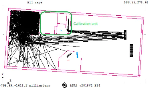
Direct paths from the calibration lamps are also prohibited and an accurate shielding is required to cope with the wide opening angle of the cone of light emitted through the entrance slits. The design of the internal calibration unit thus includes many separation walls in order to discard as much unwanted light as possible and prevent it from escaping from this part of the instrument. Specifically sized apertures also limit the angular size of the emitted calibrating beam of light. On the other hand, the zeroth diffraction order from the grating may also lead to problems. This polychromatic reflected path of light may be of high intensity and reach the detector after several interactions with the instrument walls. In our design, the rays from this straylight source follow trajectories that impact to the left side of the calibration unit where an internal panel is added to form a light trap (see Figure 7).

Figure 7. Propagation of the rays from the grating zeroth diffraction order. Light is confined at the top left after hitting the walls of the calibration unit compartment and does not reach the detector.

The ghost generated from the toroidal lens imperfect transmissivity is also studied. This second order ghost image is formed between the folding mirror and the toroidal lens. This therefore induces a divergent beam onto the detector after being reflected onto the folding mirror. Considering that an anti-reflective coating is applied on both sides of the lens, only a negligible pale veil spreads over the detector due to the internal reflections that occur through the lens.

Those considerations lead to the instrument mechanical enclosure that is shown in Figure 7. This latter features a rectangular shape into which several internal panels are included to isolate the calibration unit and the detector from multiple reflection paths. A light trap is also located next to the calibration unit to attenuate the reflected light from the grating. Eventually, grazing incidence is avoided as much as possible since this configuration may lead to the collection of photons escaping form an imperfectly collimated beam for example.

3. CALIBRATION

3.1 Spectral calibration

The calibration of the instrument requires a repeatable source featuring precise spectral lines in order to attribute to each pixel of the detector the correct wavelength. The process consists in illuminating the spectrograph entrance slit with the light of a calibration lamp that features a sufficient number of easily identified spectral lines, with wavelengths that are precisely known. Then, the pixel to wavelength matching is performed with the help of a polynomial fitting yielding a dispersion relation that enables an accurate wavelength calibration of subsequent exposures of stellar spectra.

Typical lamps used for this calibration purpose are hollow cathode lamps. These lamps are generally made up of a glass tube which contains both an anode and a cathode surrounded by a buffer gas. This latter is ionized and turned into plasma by a large voltage applied between the anode and cathode and then accelerated to eventually extract some atoms from the cathode. Collisions between the plasma and both the buffer gas and the cathode atoms induce excited atoms that will emit light after their decay to lower states.

Hollow cathode lamps commonly used for astronomical applications incorporate a buffer gas composed of several atomic species. Typical mixtures involve Thorium and Argon gases when spectral calibration is required for spectrographs operating from the visible to the infrared part of the spectrum. For example, an atlas reporting more than 2400 lines of a Th-Ar hollow cathode lamp is available for the wavelength calibration of the Cryogenic High-Resolution IR Echelle Spectrometer (CRIRES) at the Very Large Telescope27. Another atlas that covers the near-infrared spectrum from 1798 to 9180 cm-1 (i.e. from 1089 to 5561 nm) is provided by Engleman28. Other mixes of gases are also used such as Uranium-Neon when calibrating spectroscopic instruments in the near-infrared. Feasibility studies about using lamps which incorporate uranium as primary source in spectroscopic applications were realized as early as in the late sixties29. Atlases reporting spectral lines obtained with such hollow cathode lamps exist30,31 and are used as calibration sources for astronomical spectroscopy purposes32.

The choice of using a U-Ne hollow cathode lamp was made in order to calibrate our spectrograph. The selection between a Th-Ar or U-Ne hollow cathode lamp is motivated by the number of high intensity lines in the 1.0 – 1.1 µm waveband. When looking at Figure 8 where the spectra from a Th-Ar (Figure 8 (a)27) and a U-Ne (Figure 8 (b)30) hollow cathode lamps are plotted, it can be observed that very strong lines appear in the Th-Ar spectrum between 1060 and 1080 nm for example. These lines completely outshine many fainter ones, whose intensities are much lower, as can be seen when zooming onto the lower part of the intensity axis (see Figure 8 (a) bottom). This situation will likely lead to saturation of the detector for the strongest lines, while leaving the weaker ones badly underexposed. On the other hand, Figure 8 (b) reveals the same part of the spectrum that is produced by a U-Ne lamp this time. Though some strong lines are still present, their relative intensities compared to the weaker lines are much less extreme compared to the Th-Ar lamp.

(a) (b)

Figure 8. Th-Ar spectrum27 between 1060 and 1080 nm (a) and same part of the spectrum obtained from a U-Ne lamp30 (b). Bottom parts of both figures are zooms from upper ones obtained when limiting the intensity y-axis.

3.2 Flat-field calibration

Flatfield calibration consists in correcting astronomical images for the pixel to pixel variation in sensitivity. Illuminating the spectrograph with a known continuum source enables measuring those fluctuations and leads to the so-called flat-field image.

The required lamp to perform such a calibration must therefore exhibit a continuous spectrum over the considered waveband of interest, i.e. from 1 to 1.1 µm. Typical halogen lamps are used to flat-field near-infrared spectrographs as it is the case for the K-band multi-field spectrograph (KMOS) currently installed at the VLT33. A halogen lamp is therefore selected as a flat-field calibrator for the proposed spectrograph instrument.

3.3 Practical implementation

The calibration unit of the instrument is located near the optic fiber entrance and features two illuminated mechanical entrance slits positioned at symmetrical places with respect to a moving fold mirror (see Figure 9). The folded path of light connects the output end of the fiber to the collimator when the mirror stands in its down position. When calibrating, the moving mirror moves upwards and the light from the calibration box illuminates the collimator. A beamsplitter is used to collect the light from both lamps and inject it to the collimating mirror.

When observing on the sky, the light coming from the fiber output is folded to the collimator thanks to a planar mirror. This mirror stands on a translation stage that performs a vertical motion in order to approach this optical element to the fiber. The free space enables the light from the calibration lamps to reach the collimating mirror and complete both the spectral and flat-field calibrations.

Figure 9. Calibration unit optical design. Light coming from the output end of the fiber reaches a moving fold mirror when positioned in its down position and is injected to the collimating mirror during observation (right to the fold mirror, not represented in the figure). When calibrating, the moving mirror moves upwards and light from the calibration lamps is gathered with a beamsplitter and eventually goes to the collimator.

To move the folding mirror in and out of the calibration light beam we first considered a flipping mechanism. The mechanical repeatability of this component is however not sufficient to achieve the calibration accuracy needed to fulfill the scientific requirements (see Table 2). Indeed, a rough repositioning of the mirror after calibration induces a shift in wavelength measurement that must be avoided for precise calibration of stellar spectra. The comparison of the two components is represented in Figure 10.

Figure 10 (a) shows the measured wavelength across the exit slit when the flipping mirror is positioned with its maximum positioning error. The ideal case constitutes the hypothetic position that the fold mirror should exhibit in order to perfectly superpose both the hollow cathode lamp and fiber channels. Calibration is performed by injecting known wavelength into the hollow cathode lamp path and identifying them at the focal plane. The detected wavelength is measured along the entire slit length with the help of the same polynomial fitting presented in the above section concerning resolution calculations. Then, the folding mirror is perturbed by its maximum mechanical repeatability value

and the measured wavelength profile over the exit slit height is altered. Typically, the entire profile shifts vertically which induces a wavelength offset in measurements. Figure 10 (b) illustrates the same calculation when taking into account the accuracy of the translation stage.

The calibration precision specified in the scientific requirements states a value of /20. Figure 10 (a) immediately proves that the mechanical repeatability of the flipping component cannot reach such a precision. Indeed, the measured shift in wavelength rises to 2.25 times the requirement and thus the mean detected wavelength does not fall inside the acceptance zone defined by the two horizontal green lines. On the other hand, the translation stage precision leads to a wavelength error of 0.1 times the specified maximum value and the mean detected wavelength, represented by a red line, is located in the tolerated error interval (see Figure 10 (b)).

0 200 400 600 800 1000 1200 1400 1600 1049.98 1049.985 1049.99 1049.995 1050 1050.005 1050.01

Variation of PERTURBED detected wavelength across slit

Position in slit (Vertical pixels)

Wavelength (nm) 0 200 400 600 800 1000 1200 1400 1600 1049.99 1049.995 1050 1050.005 1050.01 1050.015

Variation of PERTURBED detected wavelength across slit

Position in slit (Vertical pixels)

Wavelength (nm)

(a) (b)

Figure 10. Detected wavelength along the slit length when taking into account the error on the repeatability of the flipping mechanism (a) and of the translation stage (b). The horizontal red line represents the mean detected wavelength and the two green ones are located at plus and minus the calibrating requirement from the exact injected wavelength.

4. STAR POSITIONING SYSTEM

4.1 Purpose of the instrument

When collecting the light from a telescope and feeding a spectrographic instrument with the help of a fiber, a perfect alignment of the star image with the fiber core must be achieved in order to maximize the transmitted flux to the instrument. A system must then be developed in order to be able to drive the telescope pointing and align the target image with the fiber core. To do so, both the star and the fiber core images may be visualized on a single camera and the alignment process consists in approaching both close together until they superpose.

4.2 Optical design

The proposed system is made up of a beamsplitter, a spherical mirror and a guiding camera (see Figure 11). Moreover, a back-illuminating system of the fiber is included into the spectrometer housing. This way, the fiber can be lit by its spectrograph-side output and inject light towards the telescope. To do so, a LED can be turned on and imaged onto the fiber with the help of an achromatic doublet inside the spectrograph when the fold mirror stands in its up position. The translation stage is therefore used for both calibration and star positioning processes.

The selected beam-splitting optical element is an off-the-shelf antireflective window to be used in the near-infrared waveband. This exotic choice intends to minimize the proportion of useful light, i.e. belonging to the 1 to 1.1 µm waveband, that is used for star positioning to the detriment of stellar spectra recording. This is the reason why a infrared antireflective window is selected: part of the visible star image is reflected onto the camera while the near-infrared one goes through the window and reaches the fiber input. Indeed, the anti-reflective coating of the window works fine for near-infrared wavelengths but quickly loses those characteristics when considering visible light. This part

of the spectrum is therefore prevented from propagating into the spectrograph and used for guiding purposes. Moreover, this also serves as a first “visible filter” since less luminous visible straylight pollutes the spectrograph. Due to atmospheric refraction the near-infrared and the visible images of a star may not overlap exactly. This effect will have to be calibrated during the commissioning phase of the instrument.

Once the information about the star position is known, the fiber location has to be determined in order to co-align both. This is the utility of the LED located inside the spectrograph housing which illuminates the fiber. This way, visible light is transmitted to the telescope and reaches the antireflective window. This reflected light path is then focused with the help of a spherical mirror through the window onto the camera. The fiber is now imaged onto the camera and the star-to-fiber matching can be performed.

Figure 11. Star positioning system. The instrument intends to align the observed target image with the fiber core to maximize the transmitted flux from the telescope to the spectrograph.

5. CONCLUSION

A spectrograph instrument was designed to meet the scientific requirements summarized in Table 2. Their translation into technical requirements initiated the optimization process that incorporated a toroidal lens. The purpose of the optical element was to tackle with the main aberration of Czerny-Turner spectrographs: astigmatism. The resolution driving criterion and fine analysis were then presented. The optical studies also included a straylight analysis which led to the design of the instrument mechanical enclosure and internal walls.

Other complementary units were eventually designed to provide the instrument with calibration and telescope guiding abilities. On the one hand, specific lamps were identified to perform both spectral and flat-field calibrations. On the other hand, the star positioning system is an instrument complement which was developed to locate the target image onto the fiber bundle entrance. This way, as much light as possible is transmitted from the telescope to the spectrograph for spectra recording.

As a future task, assembling and tests of the instrument will assess the validity of the previous analyses.

6. AKNOWLEDGEMENTS

This research was funded through an ARC grant for Concerted Research Actions, financed by the French Community of Belgium (Wallonia-Brussels Federation).

REFERENCES

[1] Andrillat, Y., and Vreux, J.-M., “O Stars He II and H lines in the 1 µ Region,” Astronomy & Astrophysics 75, 93-96 (1979)

[2] Vreux, J.-M., Andrillat, Y., and Biémont, E., “Near-infrared observations of galactic northern Wolf Rayet stars,” Astronomy & Astrophysics 238, 207-220 (1990).

[3] Groh, J.H., Damineli, A., and Jablonski, F., “Spectral atlas of massive stars around He I 10830 Å,” Astronomy & Astrophysics 465, 993-1002 (2007).

[4] Stevens, I.R., and Howarth, I.D., “Infrared line-profile variability in Wolf--Rayet binary systems,” Monthly Notices of the Royal Astronomical Society 302, 549-560 (1999).

[5] Short, C.I., and Doyle, J.G., “Pa-beta as a chromospheric diagnostic in M dwarfs,” Astronomy & Astrophysics 331, L5-L8 (1998).

[6] Liefke, C., Reiners, A., and Schmitt, J.H.M.M., “Magnetic field variations and a giant flare Multiwavelength observations of CN Leo,” MmSAI 78, 258-260 (2007).

[7] Schmidt, S.J., Hilton, E.J., Tofflemire, B., Wisniewski, J.P., Kowalski, A.F., Hotzman, J., and Hawley, S.L., “The First Detection of Time-Variable Infrared Line Emission During M Dwarf Flares,” American Astronomical Society 43, 21832604 (2011).

[8] Choudhary, D., Tejomoortula, U., and Penn, M.J. 2008, “Dynamics of Quiet Solar Chromosphere at the Limb,” American Geophysical Union Fall Meeting, SH23A-1622 (2008).

[9] Cuntz, M., and Luttermoser, D.G., “Stochastic shock waves as a candidate mechanism for the formation of the He I 10830-A line in cool giant stars,” The Astrophysical Journal 353, L39-L43 (1990).

[10] Dupree, A.K., Sasselov, D.D., and Lester, J.B., “Discovery of a fast wind from a field population II giant star,” The Astrophysical Journal 387, L85-L88 (1992).

[11] Kwan, J.; Edwards, S.; and Fischer, W., “Modeling T Tauri Winds from He I λ10830 Profiles,” ApJ 657, 897-915 (2007).

[12] Podio, L., Garcia, P.J.V., and Bacciotti, F., “HeI lambda 10830 line: a probe of the accretion/ejection activity in RU Lupi,” MmSAI 78, 693 (2007).

[13] Schmitt, J.H.M.M., Schröder, K.-P., Rauw, G., Hempelmann, A., Mittag, M., González-Pérez, Czesla, S., Wolter, U., Jack, D., Eenens, P., and Trinidad, M.A., “TIGRE: A new robotic spectroscopy telescope at Guanajuato, Mexico,” Astronomische Nachrichten 335(8), 787-796 (2014)

[14] Hempelmann, A., “TIGRE Telescope – General Information,” Universität Hamburg, 2013, <http://www.hs.uni-hamburg.de/EN/Ins/HRT/hrt_general_info.html> (11 May 2016).

[15] Hearnshaw, J., [Astronomical spectrographs and their history], Cambridge University Press, Cambridge, 60 (2009).

[16] McDowell ,M.W., “Design of Czerny-Turner Spectrographs Using Divergent Grating Illumination,” Optica Acta: International Journal of Optics 22(5), 473-475 (1975)

[17] Bell, R. E., “Exploiting a transmission grating spectrometer,” Review of scientific instruments 75(10), 4158-4161 (2004).

[18] Bingham, R.G., “Grating Spectrometers and Spectrographs Re-examined,” Quarterly Journal of Royal Astronomical Society 20, 395-421 (1979).

[19] Allemand, C.D., “Coma Correction in Czerny-Turner Spectrographs,” Journal of the optical society of America 58(2), 159-163 (1968).

[20] Synopsys [CODE V]. (2016). https://optics.synopsys.com

[21] Xue, Q., Wang, S., and Lu, F. “Aberration-corrected Czerny–Turner imaging spectrometer with a wide spectral region,” Appl. Opt 48, 11-16 (2009).

[22] Shafer, A.B., Megill, L.R., and Droppleman, L., “Optimization of the Czerny–Turner spectrometer,” J. Opt. Soc. Am. 54, 879–887 (1964).

[23] Xue, Q., “Astigmatism-corrected Czerny–Turner imaging spectrometer for broadband spectral simultaneity,” Applied Optics 50(10), 1338-1344 (2011).

[24] Austin, D.R., Witting, T., and Walmsley, I.A., “Broadband astigmatism-free Czerny-Turner imaging spectrometer using spherical mirrors,” Appl. Opt. 48(19), 3846–3853 (2009).

[25] Lee, K.S., Thompson, K.P., and Rolland, J.P., “Broadband astigmatism-corrected Czerny–Turner spectrometer,” Opt. Express 18, 23378–23384 (2010).

[27] Kerber, F, Nave, G., and Sansonetti, C.J., “The spectrum of Th-Ar hollow cathode lamps in the 691-5804 nm region: establishing wavelength standards for the calibration of infrared spectrographs,” The Astrophysical Journal Supplement Series 178(2), 374-381 (2008).

[28] Engleman Jr, R., Hinkle, K. H., and Wallace, L., “The near-infrared spectrum of a Th/Ar hollow cathode lamp,” Journal of Quantitative Spectroscopy and Radiative Transfer 78(1), 1-30 (2003).

[29] Rossi, G., and Omenetto, N., “Feasibility of using a uranium hollow cathode lamp as primary source in atomic absorption spectroscopy,” European Atomic Energy Community, Ispra (Italy). Joint Nuclear Research Center, No. EUR--3558. e (1967).

[30] Redman, S. L., Lawler, J. E., Nave, G., Ramsey, L. W., and Mahadevan, S., “The infrared spectrum of uranium hollow cathode lamps from 850 nm to 4000 nm: wavenumbers and line identifications from Fourier transform spectra,” The Astrophysical Journal Supplement Series 195(2), 24 (2011).

[31] Redman, S. L., Ycas, G. G., Terrien, R., Mahadevan, S., Ramsey, L. W., Bender, C. F., ... and Nave, G., “A high-resolution atlas of uranium-neon in the h band,” The Astrophysical Journal Supplement Series 199(1), 2 (2012).

[32] Sarmiento, L. F., Reiners, A., Seemann, U., Lemke, U., Winkler, J., Pluto, M., ... and Caballero, J. A., “Characterizing U-Ne hollow cathode lamps at near-IR wavelengths for the CARMENES survey,” Proc. SPIE 9147, 914754-914754 (2014).

[33] Ramsay, S. K., Rolt, S., Sharples, R. M., and Davies, R., “Calibration of the KMOS multi-field imaging spectrometer,” Proc. 2007 ESO Instrument Calibration Workshop, 319-324 (2008).