Depth-averaged flow modeling in curvilinear coordinates

Proceedings of 2013 IAHR World Congress

ABSTRACT:

A set of depth-averaged equations in curvilinear coordinates is presented. This extension of the standard shallow water equations to curved flows and to jet flows leads to a model which is very versatile. Its applicability and precision is assessed by the computation of a discharge coefficient and the nappe profiles for a sharp crested weir. Results confirm the relevance of the approach. Even if not taken into consideration in the set of equations presented here, a discussion shows that head losses could be included in the model so as to extend its application field to many civil and environmental engineering applications.

KEY WORDS: Depth-integrated model, curvilinear coordinates. 1 INTRODUCTION

The shallow water equations (SWE) have demonstrated their practical relevance for civil and environmental engineering applications, which often imply large computation domains.

The shallowness assumption states that the overall direction of the flow is known a priori. This information is used to define a direction along which the 3D Navier-Stokes equations can be integrated so as to derive a 2D model with limited precision loss. The SWE rely on the topography of the surface on which the flow propagates for the definition of an overall flow direction. The underlying topography also acts as a bottom boundary condition.

However, the underlying topography can sometimes impose abrupt changes in the local flow direction which does not correspond any more to the overall flow direction. Moreover, a flow can locally lose contact with the underlying topography and another bottom boundary condition must be imposed.

Depth-averaged flow modeling in curvilinear coordinates

Frédéric Stilmant

Professor’s Assistant, University of Liege (ULg), Hydraulics in Environmental and Civil Engineering, Liege, Belgium. Email: f.stilmant@ulg.ac.be

Raphael Egan

University of Liege (ULg), Hydraulics in Environmental and Civil Engineering, Liege, Belgium. Pierre Archambeau

Research Associate, University of Liege (ULg), Hydraulics in Environmental and Civil Engineering, Liege, Belgium. Email: pierre.archambeau@ulg.ac.be

Benjamin Dewals

Assistant Professor, University of Liege (ULg), Hydraulics in Environmental and Civil Engineering, Liege, Belgium. Email: b.dewals@ulg.ac.be

Sébastien Erpicum

Laboratory Manager, University of Liege (ULg), Hydraulics in Environmental and Civil Engineering, Liege, Belgium. Email: s.erpicum@ulg.ac.be

Michel Pirotton

Professor, University of Liege (ULg), Hydraulics in Environmental and Civil Engineering, Liege, Belgium. Email: michel.pirotton@ulg.ac.be

Civil and environmental engineering applications would take a great advantage of an extension of the SWE to curved shallow flows and jet flows because the resulting computational model would be able to include straight and curved flows as long as topography-based and jet flows in a single simulation. A unified model would thus be very versatile.

A means of achieving this extension is to refine the definition of the flow direction: instead of an overall direction, a local depth-averaged flow direction is defined at each point. This leads to the definition of curvilinear coordinates which follow the flow. Dressler (1978) initiated this approach and showed that it implied modifications in the velocity profile and pressure field. Dewals et al. (2006) extended its work to 2D configurations with a curvature in one direction and assessed the accuracy of the model when applied to a hydraulic structure. These models however rely on the bottom topography for the definition of the curvilinear coordinates.

This paper presents a set of depth-averaged equations with curvilinear coordinates having an arbitrary location within the flow. The applicability and precision of this model is illustrated for flows on weirs and jet flows.

2 MODEL

2.1 Change of variables

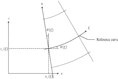
The local mass and momentum equations governing the flow are written in Cartesian coordinates (x, z). This reference frame is not appropriate for rigorous simplifications in case of flows with significant curvature. Let therefore (ξ,η) be a curvilinear coordinate system whose abscissa ξ is measured in the flow direction and abscissa η in the normal direction (Figure 1).

The definition of the curvilinear coordinate system is based on a reference curve (Figure 1) whose parametrical description is given by:

 

 

r r x x z z         (1)

This reference curve must be three times differentiable (Dewals et al. 2006). The first derivatives of the functions xr and zr with respect to ξ are given by:

 

 

cos sin r r x z        _{  }      _ _  (2)

The derivative of angle q with respect to ξ, which corresponds to the curvature of the reference curve, is written κ:       (3)

In contrast to Dressler (1978) and Dewals et al. (2006), we allow an arbitrary location of the reference curve within the flow. This curve is thus no longer linked to the bottom topography. Note that the differentiability condition can be more easily achieved with an arbitrary reference curve.

Figure 1 Definition of the curvilinear coordinates

The change of variables between Cartesian and curvilinear coordinates is defined by:





 

 





 

 

, sin , cos r r z z x x x z                _ _    _ _ (4)

The relations between partial derivatives are given by the Jacobian matrix. With definitions (2) and (3), the Jacobian matrix writes:



1





1



cos sin sin cos x z           _{ }   _{  }  _{  }      _{  }    _{ }   _    _      (5)

The determinant of the Jacobian matrix, or Jacobian, is then given by:

1

J  (6)

And the inverse relation to (5) writes:









1 1 cos sin sin cos 1 1 x z                      _{ }           _{ }       _          _ _ (7)

In case of a positive curvature, the abscissa η must remain below 1/κ for the Jacobian (6) to be positive and the change of variables to be relevant (Dressler 1978, Dewals et al. 2006). Again, the use of an arbitrary reference curve helps fulfilling this requirement.

A change of variables is also defined for the velocity components. Let (u, w) be the velocity components in directions x and z and (U, W) the velocity components in directions ξ and η. There are linked by: cos sin sin cos u U w W                        (8)

2.2 Local equations governing the flow

In Cartesian coordinates, the local equations governing a continuous flow write, with p being the pressure:

2 2 2 2 0 1 ₀ 2 1 2 u w x z u u _w u w p t x z x x w u w u p u g t z x z z w w            _  _  _ _  _                _  _  _ _  _{ }          _         _      (9)

Their transcription to curvilinear coordinates is obtained thanks to (6), (7) and (8):





 

 

2 2 2 2 0 1 1 1 _sin 2 1 _cos 2 U JW U U _{W JU} W p _g t J J J W U _U W _JU p _g W W t J                           _  _  _ _  _{ }         _{  }  _  _{ }             _{ } _  _ _{ }        _  _  _  _     _      (10)

2.2 Velocity and pressure profiles

Depth-averaging equation (10) requires assumptions on the distribution of the local unknowns (i.e. velocities and pressure) in direction η. Following Dressler (1978), we assume that

- the flow is non-rotational;

- the velocities in direction η are small compared to the velocities in direction ξ (shallowness assumption).

In Cartesian coordinates, the assumption of a non-rotational flow writes: 0

u w z x  _ _

  (11)

Its transcription to curvilinear coordinates is obtained thanks to (3), (6) (7) and (8):

 

JU W 0

 

 

 

  (12)

The shallowness assumption states that the second term of equation (12) is negligible. This leads to following velocity profile, in which the integration constant Ur is the velocity at the reference curve:



,



 

1 r U U       (13)

With equation (12) and the shallowness assumption, the momentum equation in direction η reduces to: 2 0 2 U p gz              (14)

This expression states that the energy is constant over the depth. The pressure profile can be derived from this equation. With E(ξ) an integration constant corresponding to the energy of the flow and after replacing z by its expression (4), the pressure profile writes:





 

 

 

 





2 2 1 , cos 2 1 r r U p g E z g                            (15)

(15) reduce to, respectively, a constant velocity profile and a hydrostatic pressure profile. These profiles can thus be seen as generalizations of the standard-SWE profiles.

2.3 Depth-averaged equations

Let H be the flow depth and let ηb and ηs respectively be the ordinate of the lower and upper surfaces

of the flow. Note that subscripts b and s are also used for other unknowns (velocities, pressures, Jacobians) located at the corresponding surfaces. The arbitrary location of the reference curve within the flow is denoted by the non-dimensional parameter α:



1



b s H H         (16)

Depth-integration of the stationary continuity equation in (10) gives, according to Leibnitz’s integration rule:





d d 0 s s b b U _JW              





(17) d 0 s b s s b b s s b b U U U J W J W              _{ }       



   (18)

The sum of the four last terms in equation (18) is equal to zero because of the boundary conditions which state that, at both surfaces of the flow, the local velocities are parallel to the surface (Dressler 1978). Therefore, the depth-averaged continuity equation states that the unit discharge is constant:

d 0 s b U Q          



 (19)

The expression of the unit discharge Q in direction ξ is:

1 





1 ln d d 1 1 1 s b H r r H U H U H Q H H U                  _{ }         _





(20)

In case of a stationary non-rotational flow, the momentum equation in direction ξ reduces to equation (21). Given (14), its depth-integration is trivial:

2 0 2 E U p _gz         _   _  _{  } (21) 2.4 Solving process

According to section 2.3, the unit discharge Q defined by (20) and the energy E are constant in case of a stationary non-rotational flow. With Q and E imposed as boundary conditions, the water depth H(ξ) and the reference curve (x = xr(ξ), z = zr(ξ)) can be computed step by step.

The water depth at a point at which the reference curve is known can be obtained from equation (20). To this end, let substitute the velocity Us at the upper surface of the flow for the velocity Ur at the

reference curve. The velocity profile (13) gives:





1 1

r s

U U _   H_ (22)

As the pressure at the upper surface is equal to zero, the velocity Us can then be expressed as a function of

the energy E according to the pressure profile (15):





2 1 cos

s r

U  g E z_    H _ (23)









_

_

3 1 1 1 1 1 cos 2 ln 1 1 r z Q H H E E E gE H H H H             _  _         (24)

The water depth H therefore depends only on Q, E and the parameters zr, q and κ which define the

reference curve. The value of parameter α is chosen arbitrarily and a priori.

The reference curve at a point at which the water depth is known is obtained by adding αHcosθ to the underlying topography if the bottom pressure pb given by the pressure profile (15) is positive. With

substitutions (22) and (23), the bottom pressure writes:









2 1 1 cos 1 1 1 cos 1 b r zr H E E H p z H gE E E H                _{ }    __ _    _  (25)

When the bottom pressure given by equation (25) becomes equal to zero, the flow loses contact with the underlying topography. In this case, the reference curve is obtained by solving equation (25) for κ with pb = 0. The angle q can then be deduced from definition (3) and the reference curve from equation (2).

3 APPLICATION

The aim of this application is to assess the accuracy of the model by deriving a weir coefficient from equations (24) and (25) and computing the profiles of the subsequent jet flow. The application is presented in two steps. The critical section is first identified in order to compute the discharge coefficient. The critical section is then used to initiate the computation of the upper and lower nappe profiles of the corresponding flow.

3.1 Discharge coefficient for a weir

The discharge coefficient Cd is defined by:

3 2 d Q E C g   (26)

In this definition, E’ is the hydraulic head above the weir crest zw: w

E  E z (27)

The value of the discharge coefficient Cd is imposed by the maximum discharge which can flow

through a critical section for a given hydraulic head E’. The characteristics of the critical section (xr, zr, q)

are a priori unknown. Let therefore Δz be the altitude of the lower nappe above the crest:

b w

z z z

   (28)

With definitions (26), (27) and (28), the discharge coefficient deduce from equation (24) writes:









1 1 1 1 ln ' cos 1 1 d H z H C E E E H H H H               _{ }   _       (29)

The discharge coefficient is thus a function of five non-dimensional parameters: H/E, Δz /E, α, q and κH. With definition (27), the bottom pressure pb given by equation (25) is:





2 1 cos 1 1 1 ' ' 1 b H p z z g H E E E E H               _{ }       _    _{ } (30)

The influence of the pressure profile on the discharge coefficient can be obtained by replacing (30) in (29). To this end, let define the non-dimensional parameter β as the ratio of the Jacobians at the bottom and the upper surface of the flow:





1 1 1 b s J H J H          (31)

Moreover, note that:



1



1 1 H H  _       (32)

This leads to:

 

1 cos 1 _{ln '} 1 cos ' 1 ₁ ' d b H H _E C E E z H z E E p z E E g               _  _       _ _   (33)

It appears that, for a given bottom pressure pb, the discharge coefficient Cd is no more dependent on

parameters α and κH.

The maximization of the discharge Q for a given head E’ in a critical section occurs under the constraint of the pressure that develops at the lower surface of the flow. For a sharp crested weir, the bottom pressure is:

0

b

p  (34)

In this case, the discharge coefficient is a function of three non-dimensional variables: H/E’, Δz/E’ and q. Equating to zero the derivative of Cd with respect to its first variable gives a condition on

parameter β:



_22_{1 ln}



 

_{ }2_{1 0 (35)}

Equation (35) states that parameter β is equal to 0.4685 when Cd is maximum. According to equation

(33), following relation exists between the three variables when Cd is maximum:



2



cos 1 1 ' H z E E     _ _   _  _ (36)

The discharge coefficient can thus rewrite:





ln

 

3/ 2 3/ 2 cos ' c 1 0.5216 ' 1 o 1 s 1 d _E C z z E             _  _  _  _      (37)

The discharge coefficient Cd displays no maximum when variables Δz/E’ and q vary. These

parameters are constrained by the geometry and boundary conditions of the flow over the weir.

It therefore appears necessary to identify the critical section of the flow in order to obtain the values of Δz/E’ and q. To this aim, let zb(x) describe the empirical shape of the lower nappe of a flow over a sharp

crested weir as obtained by Scimemi (1930). Hager et al. (2009) note that this profile has a maximum zb = zw + E’/9 for x = E’/4. If q(x) was a constant, the section x = E’/4 would thus be the section with the

smallest Cd, i.e. the critical section which limits the discharge flowing over the weir. As q(x) does not vary

much around x = E’/4 (where it is equal to zero), this section seems to be a good approximation of the critical section.

With Δz/E’ = 1/9 and q = 0, the discharge coefficient is:

0.437

d

C  (38)

The Rehbock formula gives a reference value of Cd = 0.4023 when zw is infinite (Hager et al. 2009).

κ of the reference curve can be deduced from equation (31) once the location of the reference curve within the flow has been chosen (parameter α).

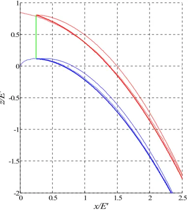
Starting from the critical section, all necessary variables are known for a step by step computation of the flow. Figure 2 compares the result for α = 0 and α = 0.5 with the profiles obtained by Scimemi (1930), as given in (Hager et al. 2009).

0 0.5 1 1.5 2 2.5 -2 -1.5 -1 -0.5 0 0.5 1

x/E'

z/

E

'

Figure 2 Upper (red) and lower (blue) nappe profiles as obtained with α = 0 (bold lines) and α = 0.5 (thin lines) starting from the critical section (green); reference profiles by Scimemi (1930) (dotted lines).

Figure 2 shows that the water depth H at the critical section is slightly overestimated. However, the nappe profiles computed with α = 0 show very good agreement with the reference. This is due to the fact that the reference curve is placed at the lower surface of the flow: in this case, the assumption θ = 0 at the section at which the computation is initiated is correct. The less good agreement of the results with α = 0.5 show that the localization of the critical section could be improved.

4 MODEL DISCUSSION

The assumption of a non-rotational flow precludes any head loss, which is too restrictive for a model which is to be used for civil and environmental engineering applications. However, the first aim of this assumption is to derive consistent velocity and pressure profiles which are required for depth-averaging the equations governing the flow. The fact that these profiles reduce to the classical profiles used in standard SWE underlines that the non-rotational flow assumption is to be seen as a working assumption: in standard SWE, the assumption of a constant hydraulic head over the depth is largely accepted, even when dissipation is taken into account in the depth-averaged equations. As already suggested by Dressler (1978), the same approach can be applied to curved flows. The assumption of a non-rotational flow would thus be used to derive the velocity and pressure profiles but not to simplify the local momentum equations in (10).

5 CONCLUSION

A set of depth-averaged equations in curvilinear coordinates has been presented. The model has been derived for stationary non-rotational flows. It is able to treat both straight and curved flows in a single approach because the local flow direction is not imposed a priori but is part of the computation. It is also able to treat both topography-based flow and jet flows in a single simulation because the bottom boundary condition is applied only after its validity has been verified. The model has been applied to the flow over a sharp crested weir. Both the discharge coefficient and the nappe profiles compare well with experimental references. The extension of the model to flows with energy dissipation has been discussed. It appears that this extension is in accordance with the approach which is classically used in SWE.

References

Dewals, B., S. Erpicum, P. Archambeau, S. Detrembleur and M. Pirotton (2006). Depth-integrated flow modelling taking into account bottom curvature. Journal of Hydraulic Research 44(6): 785-795. Dressler, R. F. (1978). New nonlinear shallow flow equations with curvature. Journal of Hydraulic

Research 16(3): 205-222.

Hager, W. H. and A. J. Schleiss (2009). Constructions Hydrauliques. Lausanne, Presses polytechniques et universitaires romandes.