Compression Based Analysis of Image Artifacts: Application to Satellite Images

(1)

HAL Id: tel-00935029

https://tel.archives-ouvertes.fr/tel-00935029

Submitted on 22 Jan 2014

HAL is a multi-disciplinary open access archive for the deposit and dissemination of sci-entific research documents, whether they are pub-lished or not. The documents may come from teaching and research institutions in France or abroad, or from public or private research centers.

L’archive ouverte pluridisciplinaire HAL, est destinée au dépôt et à la diffusion de documents scientifiques de niveau recherche, publiés ou non, émanant des établissements d’enseignement et de recherche français ou étrangers, des laboratoires publics ou privés.

Compression Based Analysis of Image Artifacts:

Application to Satellite Images

Avid Roman-Gonzalez

To cite this version:

Avid Roman-Gonzalez. Compression Based Analysis of Image Artifacts: Application to Satellite Images. Signal and Image processing. Telecom ParisTech, 2013. English. �tel-00935029�

(2)

N°: 2009 ENAM XXXX

Télécom ParisTech

école de l’Institut Mines Télécom – membre de ParisTech

T

H

E

S

E

2013-ENST-0062 EDITE ED 130

présentée et soutenue publiquement par

Avid ROMAN GONZALEZ

le 02 Octobre 2013

Compression Based Analysis of Image Artifacts:

Application to Satellite Images

Doctorat ParisTech

T H È S E

pour obtenir le grade de docteur délivré par

Télécom ParisTech

Spécialité “ Signal et Images ”

Directeur de thèse : Mihai DATCU

T

H

È

S

E

Jury

Mme. Dana SHAPIRA, Professeur, Ashkelon Acad. College Rapporteur

M. Peter REINARTZ, Professeur, DLR Rapporteur

Mme. Isabelle BLOCH, Professeur, TELECOM ParisTech Examinateur

M. Emmanuel TROUVÉ, Professeur, Université de Savoie Examinateur

M. Alain GIROS, CNES Examinateur

(3)

(4)

Compression Based Analysis of Image Artifacts: Application to Satellite Images

To my parents Gregorio Roman

Caballero and Alicia Gonzalez Rojas

with profound love

(5)

(6)

Acknowledgments

There are many people without whom this work would not have been possible. First, I would like to thank my thesis director, Mihai Datcu, who always made himself available to me and knew how to motivate me with his enthusiasm and scientific rigor. I would also like to thank Alain Giros for his advice, reviews and tips. Thank you both very much for your support.

In addition, I would like to thank Dana Shapira and Gottfried Schwarz for their advice and support during the development and revision of this work. Also, thanks to the jury for their participation in my defense and for their interest in my thesis work.

This work has been developed in three different places, so I want to thank all the members of the research groups at TELECOM ParisTech - Department TSI, the German Aerospace Center (DLR) - Remote Sensing Technology Institute (IMF), and the Centre National d’Etudes Spatiales (CNES) - AP Service for their assistance during my temporary internships and for their inspiring discussions.

I would like to give special thanks to my parents, Gregorio Roman Caballero and Alicia Gonzalez Rojas, for all their dedicated support over the years, for always being there to give me encouragement and strength to continue to move forward. Thank you to my sister Dunia Terrazas Gonzalez and my brother Jaime Terrazas Gonzalez for their support and their energy.

Finally, I want to express my thanks to Natalia Indira Vargas Cuentas and Karen Fabiola Burga Perez, on whom I could always count for their advice, encouragement and emotional support while living away from my country.

(7)

(8)

4.8 Data Compression ……….………..….………... 70 4.8.1 JPEG Compression ……….………...…. 70 4.8.2 GZIP Compression ………...………..……...…. 72 4.8.3 Delta Compression ………...…………...……...…. 72 4.9 Redundancy ………..……….………..….………... 73 4.10 Conclusions ………....…………....…………...…..….………... 73

5 Proposed Artifact Detection Methods 75 5.1 Rate-Distortion Based Artifact Detection ……….………...……... 78

5.1.1 Empirical Properties of RD for Images with Artifacts ………...…. 78

5.1.2 Artifact Classification in Error Maps ………..………...……...…. 82

5.1.3 Examples ……….……...…. 84

5.2 Normalized Compression Distance Based Artifact Detection ……...…..….. 85

5.2.1 Empirical Properties of NCD for Images with Artifacts ……….... 86

5.2.2 Artifact Classification by Similarity ………….…...………...……...…. 88

5.2.3 Examples ……….……...…. 90

5.3 New Rate-Distortion Aspects for Artifact Detection ……….... 95

5.3.1 Different Approaches for Rate-Distortion Function ………... 96

5.3.1.1 Complexity-to-Error Migration ………..…………... 96

5.3.1.2 The Kolmogorov Structure Function ………...………... 107

5.3.2 Artifact Detection with CEM ………...……...……...…. 111

5.4 Artifact Detection Using Image Quality Metrics ……….... 114

5.4.1 Empirical Analysis of Quality Metrics for Images with Artifacts …….. 114

5.4.2 Artifact Detection by Quality Metrics ………..………...……...…. 116

5.4.3 Typical Examples ………..……..………...……...…. 117

6 Analysis of Results and Quality Metrics Applications 121 6.1 Synthetic Database Description …………..………...………..…. 122

6.2 Results ………...…...………...…...………..…. 124

6.2.1 Comparison of RD and NCD Results ………...…...……... 124

6.2.2 Results of Complexity-to-Error Migration Method ……...…...……... 126

6.2.2.1 Use of Baseline JPEG and JPEG-LS ………….………... 126

6.2.2.2 Use of Baseline JPEG and ZIP ………...…………... 129

6.2.2.3 Use of JPEG 2000 and JPEG-LS ………...…….…...……... 131

6.2.2.4 Use of JPEG 2000 and ZIP ………...………...……... 133

6.2.3 Results of Existing Methods Based on Quality Metrics …………..…... 136

6.3 Conclusions for Artifact Detection ………...……...…...…….. 137

6.4 The SNCD as a Metrics for Image Quality Assessment ………...…...…….. 139

6.4.1 Database Description ………...…………... 139

6.4.2 Metrics for Image Quality Assessment ………... 140

(10)

6.4.4 Analysis of Results ………..……….………... 142

7 Conclusions and Discussion 153

7.1 Conclusions …………..………...………...………..…. 153

7.2 Discussion ………...…..……...……...…...………..…. 154

Bibliography 157

(11)

(12)

Abstract

This thesis aims at an automatic detection of artifacts in optical satellite images such as aliasing, A/D conversion problems, striping, and compression noise; in fact, all blemishes that are unusual in an undistorted image.

Artifact detection in Earth observation images becomes increasingly difficult when the resolution of the image improves. For images of low, medium or high resolution, the artifact signatures are sufficiently different from the useful signal, thus allowing their characterization as distortions; however, when the resolution improves, the artifacts have, in terms of signal theory, a similar signature to the interesting objects in an image. Although it is more difficult to detect artifacts in very high resolution images, we need analysis tools that work properly, without impeding the extraction of objects in an image. Furthermore, the detection should be as automatic as possible, given the quantity and ever-increasing volumes of images that make any manual detection illusory. Finally, experience shows that artifacts are not all predictable nor can they be modeled as expected. Thus, any artifact detection shall be as generic as possible, without requiring the modeling of their origin or their impact on an image.

Outside the field of Earth observation, similar detection problems have arisen in multimedia image processing. This includes the evaluation of image quality, compression, watermarking, detecting attacks, image tampering, the montage of photographs, steganalysis, etc. In general, the techniques used to address these problems are based on direct or indirect measurement of intrinsic information and mutual information. Therefore, this thesis has the objective to translate these approaches to artifact detection in Earth observation images, based particularly on the theories of Shannon and Kolmogorov, including approaches for measuring rate-distortion and pattern-recognition based compression. The results from these theories are then used to detect too low or too high complexities, or redundant patterns. The test images being used are from the satellite instruments SPOT, MERIS, etc.

We propose several methods for artifact detection. The first method is using the Rate-Distortion (RD) function obtained by compressing an image with different compression factors and examines how an artifact can result in a high degree of regularity or irregularity affecting the attainable compression rate. The second method is using the Normalized Compression Distance (NCD) and examines whether artifacts have similar patterns. The third method is using different approaches for RD such as the Kolmogorov Structure Function and the Complexity-to-Error Migration (CEM) for examining how artifacts can be observed in compression-decompression error maps. Finally, we compare our proposed methods with an existing method based on image quality metrics. The results show that the artifact detection depends on the artifact intensity and the type of surface cover contained in the satellite image.

(13)

(14)

Chapter 1

Introduction

The growing volume of data provided by different imaging instruments requires the use of automated tools to perform application-oriented image analysis routinely; for example, similarity detection, classification, object recognition, etc. All these analysis and interpretation steps may be affected if an image is deteriorated by artifacts. Artifacts are artificial structures being contained in an image product and represent a perturbation of the signal. The artifacts can be produced by a variety of causes. Among them are instrumental effects such as sensor saturation or A/D conversion problems. Further, aliasing effects may occur when the scene contains highly detailed structures that the imaging instrument cannot resolve properly. Finally, data processing may be another source of artifacts; typical examples are compression-decompression effects or calibration residuals.

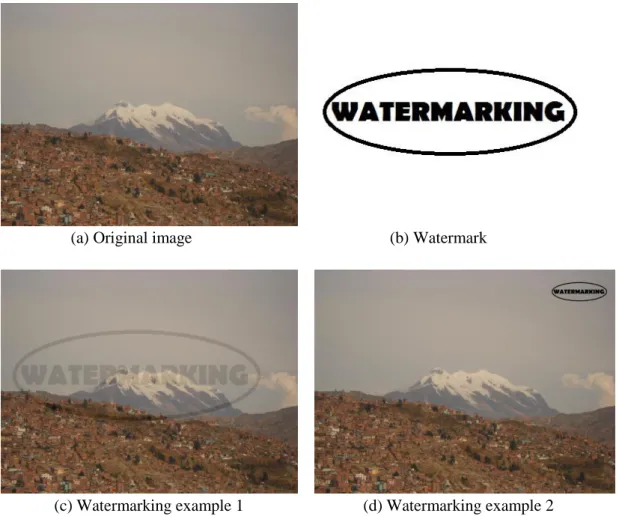
The presence of artifacts degrades the performance of image analysis, and it makes the analysis process more difficult. The presence of distortions can decrease the efficiency of interpretation and identification algorithms; it may interfere with the recognition of textures and/or the quantitative determination of features; it can also induce errors in the indexing of the images, etc. As intentional markings such as watermarks or image fakery have the same problem and affect the quality of an image, we present a comparison with other methods for image quality assessment published in the literature.

Some typical examples of artifacts are presented in Figure 1.1. In Figure 1.1 (a), we can see a line with partially inconsistent pixel values; these may be due to an intermittently stuck bit in the A/D converter. Figure 1.1 (b) shows trailing charges that sometimes occur during detector read-out. In Figure 1.1 (c), the image is affected by saturation; consequently, no radiometric detail will be available in these areas. In Figure 1.1 (d), we can see a vertical column generated by an un-calibrated dead pixel of a line scan instrument; no information is available in this column.

These artifacts perturb any subsequent interpretation process. The nature of these artifacts can be known or unknown, predictable or unpredictable; some artifacts can be described by models; however, the modeling process is sometimes very difficult. Therefore, it is necessary to implement methods being able to detect hopefully all artifacts regardless of the model which describes their formation. This thesis claims that an artifact is a more

(15)

complex or more regular region than the local environment under analysis; the artifact is uncommon when we compare many images, and it is regular itself.

A classical artifact correction approach is to create specific algorithms for each known type of artifact using a model of the artifact characteristics. There are correction methods as presented, for instance, by Jung (Jung et al. 2010) for the restoration of defective image lines; these existing methods aim at specific artifacts; however, other artifacts may remain after applying a specific correction.

(a) (b)

(c) (d)

Figure 1.1: Examples of artifacts found in SPOT images: (a) A/D conversion problems, (b) Trailing charges, (c) Detector saturation, (d) Uncorrected dead pixel creating a dark column.

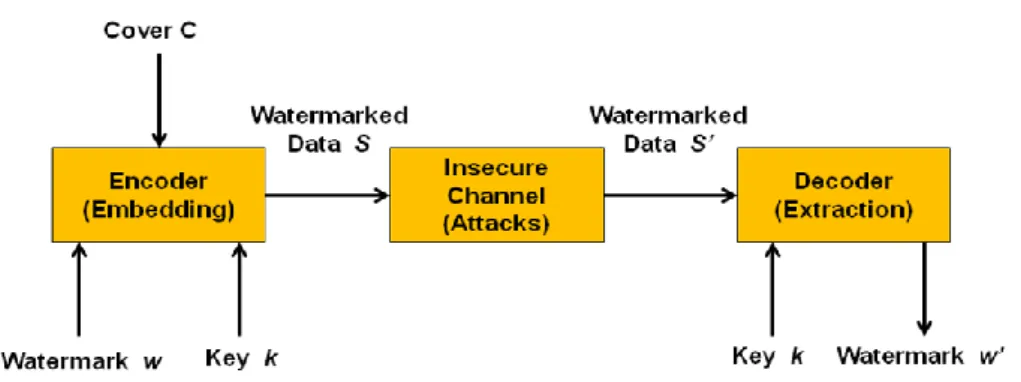
Artifacts produce changes in images, these changes are visible or not; these changes may result in an alteration of the statistics of the image or other parameters. This situation can be analyzed with image analysis approaches like presence of hidden information, or the presence of a watermark, and/or presence of super-imposed artificial structures in images. What all these image analysis approaches have in common is the analysis of changes in the statistics and information content of the image. It is for this reason that these approaches mostly use mutual information as a basis for the detection of these variations. In that sense,

(16)

the general scheme for an imaging system with artifacts is given by Figure 1.2 where S is an artifact-free satellite image; A is the distortion or artifact introduced by process Pi. The process that introduces an artifact can occur, for instance, during image acquisition, or during image processing. In this scheme, the artifact detection process is located in the processing channel and it can use an artifact model if the model is known. If the model is known, one could correct the artifact. S’ is the estimated image without artifacts if the correction process is implemented

Figure 1.2: General artifact detection scheme. S is an artifact-free image product; A is an artifact; P1 … Pn are the different processes that can introduce artifacts; I is the artifact affected image; S’ is the estimated image after artifact correction.

This thesis is a continuation of the work presented by Mallet (Mallet & Datcu 2008a), (Mallet & Datcu 2008b) and Cerra (Cerra et al. 2010). We propose the use of compression techniques both lossless and lossy compression techniques as a parameter-free method for artifact detection aiming at aliasing, striping, saturation, etc. The goal for using these compression techniques is to evaluate the level of regularity or irregularity that an artifact may have.

We propose different methods based on compression; they are presented in Figure 1.3. The first method uses lossy compression to calculate the rate-distortion function. Rate-distortion analysis allows us to evaluate how much the image data is being distorted at a given compression rate. We further develop and assess the method contained in (Mallet & Datcu 2008) based on the analysis of the compression error for lossy compression with variable compression rates. The error behavior of the image sectors with artifacts is different from the sectors that do not contain artifacts.

A second method uses lossless compression to calculate the Normalized Compression Distance (NCD); the NCD is a method proposed in (Li et al. 2004) to determine the similarity between two files using a distance measure based on Kolmogorov complexity.

As a third method we also present some approximations of the Rate-Distortion (RD) function using an approximation of the image complexity based on data compression. Here, we do not only present an analysis of the original and the compressed-decompressed image, but also an analysis of the residuals, i.e. the error between the original image and the compressed-decompressed image (Complexity-to-Error Migration). Then we obtain a multi-dimensional analysis of the distortion performance with different compression factors. These

(17)

approximate the RD curve based on complexity and can be used as a metric for evaluating the image quality.

Finally, the proposed methods are compared with an already existing method which uses image quality metrics for artifact detection based on the work described in (Avcibas et al. 2003) where the authors use image quality metrics for steganalysis.

Figure 1.3: Artifact detection methods.

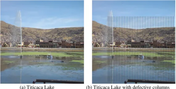
In order to evaluate the various proposed methods, we use a database with synthetic artifacts to analyze the success rate of detection depending on the intensity of the artifact. We use cloud-free images without haze effects in order to avoid problems related to atmospheric phenomena.

The thesis is structured as follows: Chapter 2 presents basic aspects of optical remote sensing and we demonstrate typical artifacts encountered in remote sensing images. Chapter 3 shows similar problems in other application areas. In Chapter 4, we present an overview about information theory, entropy and complexity. Chapter 5 presents new methods for artifact detection based on rate-distortion analysis, artifact detection based on Normalized Compression Distance, - - artifact detection based on image quality metrics. In Chapter 6, we show results and quality metrics applications. Conclusions are contained in Chapter 7.

(18)

Chapter 2

Basic Aspects of Optical Remote

Sensing

Formally speaking, remote sensing deals with extracting information about a remote object. In our case, however, remote sensing is understood as a common measurement technique for airborne or space-borne instruments observing the Earth (Malacara & Thompson 2001). Prominent examples are satellites carrying optical imaging instruments (i.e., space qualified cameras). A typical scenario is shown in Figure 2.1; here, the Sun illuminates the surface of the Earth, while a satellite equipped with a camera is taking images. The digitized image data will then be transmitted from the satellite via a radio link to a ground station on Earth that receives the image data. There, the image data will be further processed, calibrated and interpreted.

Figure 2.1: Image acquisition by a remote sensing platform [EGI – Energy & Geoscience Institute]

When we acquire images as shown in Figure 2.1, our source of energy is the Sun. The sunlight traverses the atmosphere and is reflected by the surface of the Earth. A fraction

(19)

of the overall sunlight will then be collected by the camera aboard the satellite. Apart from the sunlight finally being collected by the instrument, much sunlight will be scattered (i.e. re-directed) and absorbed by various physical processes in the atmosphere and on ground.

2.1 Principles of Electromagnetic Waves

The reflected sunlight seen by the instrument will comprise various wavelengths as shown in Figure 2.2. In principle, we can observe the electromagnetic spectrum from shorter wavelengths (< 10-5 μm) to longer wavelengths (> 106 μm). Common optical remote sensing techniques use several regions of this electromagnetic spectrum for different applications.

Figure 2.2: Electromagnetic radiation, from shorter wavelengths (< 10-5 μm) to longer wavelengths (> 106 μm).

For our applications, we mainly consider the visible and infrared spectrum. The visible spectrum has a wavelength range from approximately 0.4 to 0.7 μm (from violet to red). This range is the portion of the spectrum that comprises the visual colors seen by a human observer. Apart from that, the ultraviolet portion of the spectrum is useful for optical remote sensing of the Earth’s surface because some rocks and minerals fluoresce when they are illuminated by ultraviolet radiation (Note that most of the ultraviolet radiation is absorbed by the atmosphere making the fluorescence effects of the land cover invisible to a space-borne instrument). Another range of the spectrum of interest is the infrared region from approximately 0.7 μm to 100 μm. The infrared region can be sub-divided into three regions with different properties: the near-infrared, the mid-infrared, and the far-infrared region. The near-infrared region ranges from approximately 0.7 μm to 2.5 μm; this range is often used to characterize vegetation. The mid-infrared region extends from approximately 2.5 μm to 10 μm; this range is mainly used for the detection of high temperature events like fires or volcano eruptions (the emitted radiation is not a direct reflection of the incident sunlight; the emissions can also be measured on the night side of the Earth). The far-infrared range from approximately 10 μm to 100 μm is used for thermal radiation budget measurements of the Earth and is also not a direct reflection of the incident sunlight.

(20)

However, in remote sensing of the Earth’s surface we cannot use the full optical spectrum as many spectral regions are masked by atmospheric absorption. The sunlight has to traverse the Earth’s atmosphere where particles and gases will affect the radiation due to scattering or absorption. Scattering means a redirection of the photons due to their interaction with particles and gaseous molecules. On the other hand, absorption is a phenomenon where molecules in the atmosphere absorb energy at various wavelengths. In Figure 2.3, we can see a plot of the atmospheric absorptions produced by water vapor and carbon dioxide. The water vapor and the carbon dioxide contained in the atmosphere produce pronounced absorption features mainly around 1.4 and 1.9 µm; these absorptions reduce the reflected energy almost completely, so an optical remote sensing instrument operated in these regions could not get much information about the surface of the Earth.

Figure 2.3: Atmospheric absorptions for electromagnetic wavelengths produced by water vapor and carbon dioxide.

2.2 Data Acquisition and Data Reception

Before we deal with artifact detection in optical satellite images, we have to understand the basic image acquisition and processing chain of a classical satellite camera. It collects the electromagnetic radiation entering the instrument and a semiconductor detector (carrying a line or a matrix of “picture elements” = pixels) converts the electromagnetic radiation into electrical signals for each pixel. The electrical charges of the pixels are then read out, amplified and digitized into “digital units” (i.e. brightness counts). The digitized data are then transmitted to a ground station. Within the chain we have to be aware of a number of mostly instrumental effects that may affect and degrade the quality of the acquired images. When the effects have known causes, they can be grouped and called artifacts.

Based on the concept illustrated in Figure 2.4 and Figure 2.5, one can then see where typical artifacts may be introduced into the image generation and processing chain.

(21)

Figure 2.4: Basic image acquisition and processing chain of a classical satellite camera; we can see where typical artifacts may be introduced into the image generation and processing chain (space segment).

(22)

Figure 2.5: Basic image acquisition and processing chain of a classical satellite camera; we can see where typical artifacts may be introduced into the image processing chain (ground segment).

(23)

For nearly each of the major components shown in Figure 2.4 and Figure 2.5, there exist typical risks to include artifacts (i.e., effects that cannot be modeled by simple additive Gaussian noise sources). Interestingly, one of the few system components that preclude artifacts is the data transmission link between the satellite and the ground station. Here, the use of modern error recognition and correction codes guarantees a near perfect data transmission provided that the data link is not interrupted and has a sufficient signal-to-noise ratio. As we have sufficient expertise about the nature and the typical characteristics of most of the potential artifacts we can address the problem of identifying them routinely. This will be demonstrated in the next two chapters.

The keywords contained in Figure 2.4 and Figure 2.5 are explained in more detail in Table 2.1. For each optical/electronic component of a satellite camera system we list the typical artifact-prone effects, explain their causes and effects, show what type of technology is most affected by this kind of artifact, and assess the importance and correctability of the effect. Component Artifact and Effect Explanation Critical Technology Importance Correctability Sun Photon noise The solar photon flux

fluctuates obeying an arrival process: Photon noise = square root of the number of photons. This effect is independent of the instrument design and its implementation technology.

The effect yields a basic assessment of the signal-to-noise behavior of an optical system.

Stacking of highly similar images may yield higher signal-to-noise results (for low light level images). Solar

elevation

The solar elevation determines the amount of photons actually impinging on a unit area on ground. The solar elevation depends on the date and the target area location. This effect is independent of the instrument design and its implementation technology.

The analysis of time series data requires elevation corrected (i.e. inter-comparable) data.

Simple trig formula; the required parameters may be taken from image metadata or computed based on date, time, and location. Sun-to-Earth

distance

The actual Sun to Earth distance affects the image brightness.

This effect is independent of the instrument design and its implementation technology.

For image time series data this is a 3% effect. Simple one-line correction formula approximating the actual distance versus date. Atmosphere Absorption A sizeable percentage

of the photons of a given wavelength will be absorbed. The actual absorption depends on the spectral region, the air pressure, temperature, and trace gases such as water vapor and aerosol content of the atmosphere.

One should avoid heavily affected wavelength regions.

The severity of the phenomenon depends on the spectral region. A high quality modeling of the actual absorption parameters is a demanding task and does not yet correct the effects.

Scattering See “Absorption” Avoid imaging in the blue.

Important for bad contrasts in the blue and for conversion to surface

reflectances (if any).

A high quality modeling of the lost and gained signal components is a demanding 3D task and may be not yet a remedy.

Clouds and their shadows

Clouds prevent imaging of the surface. Cloud shadow regions have a low signal level.

Some instruments provide cloud flags within their higher level products. Clouds prevent surface classification. Disregard affected regions (this requires precise cloud annotation in the image product).

(24)

Compression Based Analysis of Image Artifacts: Application to Satellite Images Component Artifact and Effect Explanation Critical Technology Importance Correctability Atmosphere Haze Haze degrades the

image contrast and destroys fine details.

Avoid imaging under hazy conditions.

Important in image time series with different haze levels (this makes inter-comparisons difficult).

One can apply contrast enhancement; however, this may introduce new artifacts (e.g., near edges in images). Aerosols Aerosol effects may

range from image contrast reduction to sandstorm imaging. Avoid aerosol imaging or determine aerosol parameters.

See above See above

Imaged Surface Area

Absorption Reduces the surface brightness of some materials. This effect is independent of the instrument design and its implementation technology. Allows surface classification. Shall not be corrected for (needed for image interpretation).

Scattering Reduces the surface contrast.

See above Mostly of minor severity Shall not be corrected for. Bi-directional reflection [distribution] function (BDRF)

The observed surface brightness depends on the local illumination/ observation geometry. Avoid imaging with sub-optimal geometries. Could become important for instruments with highly agile pointing. A correction would require a reliable knowledge of the physical parameters. Shadows May prevent correct

surface classification.

Does not depend on the instrument technology (besides contrast fidelity).

Depending on scene details and terrain shape.

Could be required for conversion to surface reflectance.

Occlusions Some surface details may be not visible due to a slant viewing geometry. Avoid slant viewing in highly structured terrain. Important in special cases only. Not correctable

Baffle Stray light The baffle shall reduce stray light from non-target directions. There is always a conflict between the desired baffling capabilities and the baffle size.

Images with stray light from sunlit snow surfaces might be degraded.

A full stray light correction is difficult (needs modeling). Optics Modulation transfer function (MTF) Focus Aberrations

Sharp transitions are smoothed by the transfer function of the optics, the actual resolution depends on the focusing, and some additional aberrations may be introduced.

Some low pass filtering is often a design goal; after the launch of a spacecraft we often have unwanted mechanical mis-alignments of optical systems. Color aberrations are most often uncritical.

MTF effects in remote sensing are only critical if we are interested in extremely small details. In principle, MTF effects can be inverted but a correction often introduces new artifacts (e.g., ringing). Spectral filters Transmission curve Leakage Reflections

Each spectral filter has a pass-band and shall block all other colors. Some filters show spectral leakages and cause unwanted multiple reflections.

Some desired filter shapes are difficult to produce in space qualified technology. The filter aging characteristics and their reflection behavior has to be tested carefully. The analysis of multi-spectral images often relies on differences between spectral bands.

Any color correction is rather difficult and calls for extensive modeling.

(25)

Compression Based Analysis of Image Artifacts: Application to Satellite Images Component Artifact and Effect Explanation Critical Technology Importance Correctability

Detector(s) Type and operations Responsivity Dark current Blemishes Thermal noise Blooming Transfer efficiency Residual image Ghost images Saturation Color band displacement

Visible sensor artifacts depend on the sensor type, the image recording and the read-out concept (e.g., residual images caused by CMOS detectors, smearing caused by TDI recording, and artifacts due to read-out with on-going illumination). The most visible artifacts are due to non-uniform pixel responsivity, non-uniform dark current signatures, thermal noise, blooming of bright targets, insufficient transfer efficiency during sensor read-out, existence of residual images, or ghost images due to unwanted reflections, saturation of extended areas, or geometrical displacements between color sensors. Improvements in sensor technology have improved the situation considerably. Sensor butting has become less important; dead or hot pixels, blemishes and striping can be avoided by careful sensor selection. A camera design with reduced read-out speed will reduce the noise level. Detector overflow calls for appropriate camera operations. The quantitative analysis of digital images calls for artifact-free sensor signals as they distort the recorded scene.

A lot of experience is available how to calibrate sensors with respect to pixel and read-out signatures, how to correct single pixel blemishes by interpolation, and how to characterize thermal noise and residual images. Read-out electronics Linearity Zero level stability Low pass effects Cross-talk Multiplexing effects Noise effects The read-out electronics (and its amplifiers) can add additional artifacts to an image: amplifiers will not be perfectly linear in a thermally varying environment, their zero level may drift, and random noise will be introduced.

The critical point is to design high-speed electronics with low noise.

The most important detail is the fidelity of multiple (i.e., parallel) read-out channels. Each channel needs similar thermal responses. Linearity, zero levels and low pass effects have to be verified in detail and can be calibrated as systematic effects. In contrast, cross-talk and noise effects often cannot be treated as systematic effects and remain difficult to correct for. A/D converter Linearity Zero level Stuck bits Quantization noise Any technical imperfection during A/D conversion will generate image artifacts.

The A/D converter has to fast enough, shall be linear, and shall not be prone to stuck bits. The transformation of analogue signals into quantized steps will introduce quantization noise that depends on the quantization step size.

The A/C converter quality affects each pixel of every image. Therefore, a good design is very critical.

A known non-linearity can be calibrated. A good zero level stability can be reached via correlated double sampling. Stuck bits need special software tools and quantization noise has to be taken for granted.

(26)

Compression Based Analysis of Image Artifacts: Application to Satellite Images Component Artifact and Effect Explanation Critical Technology Importance Correctability Data compression Compression losses On-board data compression prior to transmission to ground allows high volume imaging. However, high rate compression causes compression effects (e.g., so-called blocking effects).

Existing data compression techniques (e.g., JPEG type image compression methods) have to be applied in a way not to degrade the image data too much. The analysis of the image content must not be compromised. This can be verified by studying the histograms of images after de-compression.

It is important to select a set of compression parameters that do not falsify the image content to be interpreted. A clever selection of the compression parameters necessitates a lot of test runs with typical examples.

There exist some enhancement methods for the reduction of blocking effects. However, these methods create new problems as they degrade image details. On-board data handling Storage capacity Comfortable imaging needs sufficient storage capacity to store images prior to downlinking them to ground. Otherwise, we are faced with interrupted imaging (the ultimate “artifact”).

Nowadays, technology for on-board digital data storage is available.

The data rate produced by an imaging instrument has to be designed in accordance with the data transmission capabilities of the satellite.

One can try to optimize the parallel or sequential operations of all data generating instruments aboard a satellite. Formatting and error correction coding

(none) Nowadays, powerful error protection coding is available that provides either perfect data quality or a loss of data. This technology has become an integral part of data transmission and is no longer critical. Error protection is a pre-requisite for the transmission of compressed data (e.g., images). Existing software packages with a proven record should be used. Data transmission and reception Antenna gain Antenna pointing Amplifier cooling Receiver synchronizati on

(The data analysis community is not involved in this field of activity.)

(not for data analysts)

Data re-formatting

Data gaps (see above) (see above) (see above) (see above) Data

de-compression

Decompres-sion noise

Software packages being used for decompression may include selectable optimization parameters.

(27)

Compression Based Analysis of Image Artifacts: Application to Satellite Images Component Artifact and Effect Explanation Critical Technology Importance Correctability Radiometric correction Calibration concept Detector and read-out effects Conversion to radiances Conversion to reflectances Calibration residuals Common radiometric calibration concepts contain a signal correction part for known instrumental effects, and routines for the conversion of (corrected) detector counts into physical units (radiances and/or reflectances). Uncorrected effects appear as artifacts. The long term monitoring of the calibration quality may use statistics of residual errors. The signal correction part and the conversion steps are dynamic processes: after an initial on-ground calibration, in-flight calibration experiences lead to improved methods and results. Often, one faces new calibration problems during the lifetime of an instrument. A proper radiometric correction is a basic pre-requisite for quantitative image analysis and interpretation. Improperly calibrated images may lead to wrong conclusions. As a rule, known instrument characteristics that can be corrected with acceptable implementation effort will be contained in common radiometric correction packages. On the other hand, one can never expect a perfect radiometric calibration. Geometric correction Rectification approach Geo-coding accuracy Re-projection effects Terrain effects Geometric correction packages re-project radiometrically corrected images onto a (sometimes selectable) common map projection. (This topic is of secondary importance in this dissertation and we will not provide too many details here.)

One can use rectification approaches ranging from tie-point and interpolation techniques to highly accurate rational function models and additional support by existing DEMs. The selected method determines the kind of artifacts generated during the rectification. Important points to consider are the accuracy of available geo-data, re-projection artifacts, and the handling of terrain effects.

Geometrically corrected images are required for applications that need absolute locations of objects, or the comparison of locations in data of different instruments, etc. Some geometry routines allow the interactive selection of tie-points. The use of additional tie-points may reduce local blunders. Higher level products Algorithmic stability Derived quantities in higher level products may be imprecise (for instance, vegetation parameters derived from multi-spectral images). The transformation of basic image products into derived physical quantities needs appropriate algorithms (that are not always available or of good quality).

The acceptance of higher level products by the user community hinges on their correctness.

Comparisons with ground truth measurements can give clues to the quality of the used algorithms but ground truth measurements are not always available.

(28)

On the other hand, if the available image data are not affected by too serious artifacts, the image content can be analyzed and interpreted. Besides the recognition of spatial objects (such as a road or a bridge) in an image, one can in the case of a camera with sufficiently many separate spectral channels also use the shape of a spectral curve to identify and distinguish different materials. For example, vegetation has a high reflectance in the near-infrared range, in contrast to inorganic materials (e.g., rocks) that have specific absorption bands that we can use to detect the presence of minerals. This is illustrated in Figure 2.6.

Figure 2.6: Typical spectral signatures; for example, vegetation has a high reflectance in the near-infrared range, in contrast to inorganic materials (e.g., rocks) that have specific absorption bands that we can use to detect the presence of minerals.

The imaging scenario given above has to be discussed in conjunction with the resolution capabilities of a camera. The resolution of a camera can be defined as its spatial resolution (i.e., the capability to discriminate two adjacent point targets), its radiometric resolution (i.e., the capability to discriminate two similar brightness levels), its spectral resolution (i.e., the capability to discriminate two similar colors) and its temporal resolution (i.e., its capability to resolve temporal changes in image time series. These four kinds of resolution will be explained below in more detail.

2.2.1 Spatial Resolution

The spatial resolution of an optical instrument is basically constrained by the size of a detector pixel, the focal length of the camera optics, the distance from the satellite to the target, and the assumption that all neighboring pixels are immediately adjacent. Then these parameters define the nominal footprint of a detector pixel projected onto the surface of the Earth. This footprint size can be used to determine the capability to resolve two adjacent point targets. However, the footprint is defined for an ideal instrument; in practice, the atmosphere may blur the image, the camera optics has a defined transfer function, the detector and its read-out electronics may act as low pass filters, etc. As an additional complication, the term “spatial resolution” is often confounded with the pixel spacing used

(29)

for the representation of an image product. The actual pixel spacing used in a digital image – for instance, after a geometric re-projection – may correspond to a pixel grid that differs considerably from a grid commensurate with the ideal spatial resolution.

2.2.2 Radiometric Resolution

The radiometric resolution of a camera is limited by the number of bits provided by the A/D converter that quantizes the electrical charges (i.e., the electrons) of a detector pixel (after read-out and amplification) into digital units. Of course, this limitation is not yet a fully valid criterion: We also must be sure that the lower bits of the A/D converter do not only contain noise but useful information. Otherwise, we would have a nominal radiometric resolution that does not fulfill its promises. Other points to consider are the full-well capacity of the detector pixels and the setting of the read-out amplification factor prior to A/D conversion. The amplification factor has to be selected according to the signal level, the signal dynamics, and the quantization capabilities of the A/D converter.

2.2.3 Spectral Resolution

The spectral resolution of a remote sensing instrument is determined by the number of individual spectral bands that the sensor(s) can detect and handle. Classical remote sensing cameras have four or more spectral bands: at least a red band, a green band, a blue band, and an infrared band; there are also instruments which produce multispectral images that have approximately 10 to 15 bands. In addition, there are also hyperspectral imagers that provide more than 100 spectral bands. From a technical standpoint this means that either individual detectors are available for each spectral band (a classical design approach with sometimes displaced viewing directions for each spectral band), or a detector provides on-chip color band discrimination (for instance, a so-called Bayer type image sensor), or – in the case of hyperspectral instruments – a prism generates a multi-element color spectrum for each single point target on ground to be recorded as a full sensor line (the “imaging spectrometer” concept). Within this framework, we have to consider that the technical solution adopted for a specific camera has to provide a reasonable signal-to-noise level: narrow spectral bands have a lower signal level than broader spectral bands. The lack of sufficient energy can only be compensated by longer exposure times; however, the ground-track motion of the satellite and the read-out strategy of the detectors constrains the admissible exposure times.

2.2.4 Temporal Resolution

When a satellite is orbiting the Earth on a (near-) polar orbit, also the Earth is rotating about its axis. While a typical satellite orbit has an orbit period of about 100 minutes, the Earth requires 24 hours for a full rotation. This means that after a full satellite orbit cycle, the Earth has rotated by more than 20 degrees and our new satellite ground track will be displaced form the previous one accordingly. Thus, it takes some time until the same location on the Earth’s surface can be imaged again. This re-visit time period (usually several days) limits the temporal resolution of a satellite camera. The actual temporal resolution of a camera

(30)

system depends on more factors, including the lateral (off-nadir) pointing capability of the camera to re-acquire the same location again by slant viewing, the swath width of the sensor and its desired overlap, and the geographical latitude of the target area: Near the equator the longitudinal inter-track spacing is greatest; near the poles, it is minimal, but we also have to take into account that cloud cover could make a number of image takes unusable and this could lead to a degraded temporal resolution.

2.3 Earth Observation Image Information Content and Quality

In this section, we will describe the information extraction from satellite images and the importance of image quality for satellite images. We will also study in more detail the artifacts introduced in Section 2.2 and their influence on information extraction.

We concentrate on the information that one can extract from these images in order to interpret and apply this information in different fields. Here, the image quality plays an important role. If we want to get the highest amount of information from an image, we need to have a good image quality.

This is a pre-requisite for the detection, measurement, identification and interpretation of different targets. Targets in remote sensing images may be any feature, object, texture, shape, structure, spectrum, or land cover being contained in the image.

Data processing and analysis in remote sensing can be performed either manually or automatically. Currently, there are many research groups that develop automated tools to detect, identify, extract information and interpret targets without manual intervention by a human interpreter.

2.3.1 Information Content

To extract the information contained in satellite images, one has to extract different characteristics such as color, texture or shape.

Color features based on spectral information can be used to extract information from multi-band image pixels for analysis, classification, indexing, segmentation, etc. A typical example is the analysis and comparison of spectral signatures.

Another way to extract information from an image is using its texture. In general, texture is defined as a segment with homogeneous properties or characteristics; it represents a repetition of motifs that create a visually homogeneous image maintaining a spatial relation. There are many researches in this field to characterize the different spatial relationships and evaluate the amount of information that can be extracted from satellite images as shown in (Dowman & Peacegood 1989). For instance, Haralick et al. 1973 used statistical measures to discriminate the different structures in an image; the authors propose 14 features calculated from a co-occurrence matrix corresponding to the second-order statistics of pixel neighborhoods.

The extraction of shape information is based on geometric characteristics such as area, eccentricity, longitude axis, invariant algebraic momentum, etc.

It is also possible to combine spectral, texture and geometric characteristics for the analysis of satellite images that results in extracted features.

(31)

Figure 2.7: Example of remote sensing image analysis [International Charter on Space and Major Disasters].

After a feature extraction process, a classification step is performed; for classification, one can use supervised or unsupervised classification. Supervised classification needs data for training; one needs a good selection of training data with relevant and appropriate samples to obtain an optimal parameterization. The parameters that are the result of the training step are then used for the final classification of the remaining data.

In contrast, unsupervised classification does not need a training step. This type of classification uses clustering algorithms to determine the grouping of the data. The type of algorithm determines which features will be the most predominant ones for clustering either color, texture or shape. In most cases, however, one has to specify the number of data clusters, the selected distance parameter, etc.

Whatever classification type will be used, the final result of the analysis process is a mosaic either composed of pixels or image patches in which each element represents a category of interest.

(32)

2.3.2 Earth Observation Image Quality

A satellite image must comply with the needs of end users, thus the required quality of the image depends on the type of application, which could be photo-interpretation, forest and deforestation monitoring, agricultural land monitoring, meteorology, water color analysis, monitoring of natural disasters (earthquakes, floods, etc.), defense applications, etc.

Generally, there are well-known criteria to evaluate the quality of a satellite image in three important domains: Geometric quality, radiometric quality, and quality aspects related to the actual resolution.

In the geometric domain of images, where the interesting topic is to determine the position of the pixels with high accuracy, the criteria to define the image quality have to evaluate the preservation of locations and distances, including the precise overlapping of color bands, and accurate heights.

In the radiometric domain, the important thing is the brightness level of each pixel; the criteria to be evaluated are the calibration accuracy, the radiometric noise, etc.

In the domain related to resolution, the important issues are the resolution capabilities, and the perception and reproduction of details; the topics which must be taken into account for the quality assessment are the sampling technique, the modulation transfer function, etc.

These criteria for assessing the quality of a satellite image serve to define the specifications of different components for an Earth observation project and to assess its capabilities to satisfy the user needs.

2.3.3 Earth Observation Image Artifacts

In the literature, we found no standard definition of an image artifact. Therefore, we had to find a definition based on our experiences. As will be shown in Section 2.3.4 in more detail,

- We define artifacts as artificial structures that represent a structured perturbation of the signal.

In most cases, these artifacts are produced by the instrument; for instance, technical design problems, saturation of the sensor, or on-board signal processing. Therefore, these artifacts induce errors during image analysis.

In the following, we will describe typical artifacts that may occur (or have been simulated) in images that were taken by the SPOT 5 instrument, by IKONOS, by MERIS, and by the hyperspectral instrument ROSIS. Each of these instruments is prone to typical artifacts. Therefore, we begin with a short survey of each instrument and its critical components.

SPOT 5 (launched in May 2002) represents a classical optical line scan instrument with 60 km swath width that has a long heritage of predecessor instruments dating back to SPOT 1, SPOT 2, etc. The polar and sun-synchronous orbit of SPOT 5 is characterized by its mean height of 822 km, its period of 101 minutes and its equator crossing time (on its descending branch) of 10:30 AM local time. The orbit repeat cycle of 26 days (combined with off-nadir imaging) allows a re-visit period of a target area within typically 2 to 3 days.

(33)

SPOT 5 carries two camera instruments to be considered here: HRG and HRS. (The SPOT 5 payload also comprises an optical vegetation monitoring instrument that is not considered here.) HRG represents a typical multi-color instrument with a high resolution panchromatic channel (2.5 or 5 m resolution) and four additional color channels with lower resolution (10 m or 20 m resolution). All channels are recorded by line sensors. HRS is a stereo pair generating instrument delivering simultaneously acquired and geometrically overlapping forward and backward looking strip images. The image strips acquired by CCD line sensors (via push-broom technology) have a panchromatic resolution of at least 10 m and a swath width of 120 km and can be used to generate digital elevation models.

The A/D conversion of SPOT 5 delivers 8 bits per sample. This should allow us to see persistent artifacts that are not due to an excessive signal amplification and quantization.

When we concentrate on potential artifacts of the HRG instrument, we can expect to see all typical features of a classical multi-spectral push-broom instrument such as residual detector blemishes and discrepancies between the individual color bands. As SPOT 5 can be considered as a typical “workhorse instrument”, also the SPOT 5 artifacts should be very typical of this type of instruments. Thus, SPOT 5 images are a good choice for studying artifacts in satellite images.

Another instrument is IKONOS, a very high resolution push-broom imager: IKONOS was the first commercial sub-meter resolution satellite to acquire panchromatic image strips with 0.82 meter resolution and multispectral images with 3.2 meter resolution. The high resolution is reached by its telescope focal length of nearly 10 m and represents the state of civilian technology of 1999 that developed further, of course, during the last years (e.g., into the Pleïades or WorldView satellite series).

The polar and sun-synchronous orbit of IKONOS is characterized by its mean height of 681 km, its period of 98 minutes and its equator crossing time (on its descending branch) of 10:30 AM local time. This, together with the off-nadir pointing capabilities of the spacecraft, and an instrument swath width of 12 km allows a revisit period of a target area of about 3 days. The downlinked image data can be acquired by several ground stations around the world that can be operated independently from each other.

IKONOS provides simultaneously recorded panchromatic and multispectral image strips via separate line detectors: a panchromatic CCD detector with 13,500 cross-track pixels (operated in TDI mode), and 4 photodiode color detectors with 3375 cross-track pixels. The color separation is accomplished by multi-layer spectral filters on glass. Besides its high geometrical resolution, IKONOS also provides a high radiometric resolution: The A/D converter delivers quantized data with 11 bits per sample. These data will be compressed via adaptive differential Pulse Code Modulation with a compression rate of 4.25.

As a result of these demanding design parameters, one can expect typical geometrical and brightness artifacts due to the very stringent spatial and temporal imaging requirements such as contrast degradations, residual TDI mismatch, etc. A critical issue is the attainable image classification accuracy.

Finally, we will also consider the MERIS instrument, an imaging spectrometer operating in the visible and near-infrared spectral range from 390 nm to 1040 nm. From this overall spectral range, one can select 15 spectral bands by ground command.

MERIS was flown aboard the now defunct ENVISAT satellite with the following orbit parameters: polar sun-synchronous orbit with a mean height of 800 km, a period 101 minutes and an equator crossing time (on its descending branch) of 10:00 AM local time. These parameters yield a repeat cycle of 35 days.

(34)

One of the most important points for artifact detection is the wide cross-track field of view of the MERIS instrument covering 68.5° requiring a polarization scrambler and resulting in a swath width of 1150 km; technically, this wide field of view is accomplished by installing five identical optical modules arranged in a side-by-side configuration. As each module has to be calibrated individually, small residual offsets among the calibration parameters of a module will immediately cause visible offsets in image mosaics.

Within each optical module, MERIS uses a separate frame detector with an imaging zone of 740 spatial × 520 spectral pixels. Each frame detector consists of a CCD where the spatial information is recorded in an image row (following a classical push-broom imaging concept), while the spectral content of a push-broom row is mapped along the columns of the CCD. This concept necessitates elaborate read-out strategies that result in spectra with a high signal-to-noise ratio. One can imagine that a number of potential read-out artifacts may jeopardize the quality of the spectra. The radiometric quality of the data is preserved by an A/D conversion with 12 bits per sample. This high resolution necessitates elaborate calibration concepts that are of course again prone to artifacts. Therefore, MERIS data are a prime target for artifacts appearing as small but sometimes annoying spatial and/or spectral details.

ROSIS (Reflective Optics System Imaging Spectrometer) is a hyperspectral airborne instrument; it has 115 spectral bands in the range from 430 to 860 nm with 14 bits of radiometric resolution. Typical artifacts for this class of instruments are radiometric calibration errors due to insufficiently corrected atmospheric effects (e.g., water vapor profile residues).

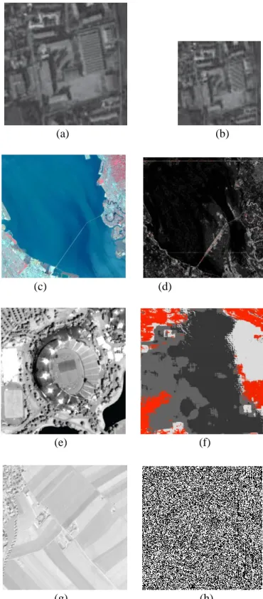
Figure 2.8 shows some examples of artifacts, in (a) and (b) we can see texture changes due to aliasing; (c) and (d) show the existence of horizontal lines which could be erroneously detected as bridges; (e) shows saturation, and (f) shows blocking effects; (g) and (h) contain strips of the 21 bit in one band of the hyperspectral image. These artifacts may interfere with the recognition of a texture, target identification, land cover segmentation or the quantification of features. The nature of some of these artifacts is mostly known; however, these artifacts cannot be described by a single model; that is why we aim to detect these artifacts regardless of the specific formation model, i.e. we look for parameter-free methods.

(35)

Compression Based Analysis of Image Artifacts: Application to Satellite Images (a) (b) (c) (d) (e) (f) (g) (h)

Figure 2.8 Typical examples of artifacts: (a) and (b) Change of texture by aliasing after processing. (c) and (d) Horizontal lines appearing after contrast enhancement (e) Sensor saturation. (f) Blocking effects. (g) and (h) contain strips of the 21 bit in one band of the hyperspectral image.

(36)

(a) A/D conversion problem (SPOT) (b) Trailing charges

(c) Saturation (d) Dead column

Figure 2.9: Some examples of our artifact database: (a) A/D conversion problem (SPOT) (b) Trailing charges. (c) Sensor saturation. (d) Dead column.

In the following, we present and describe some specific actual artifacts found in satellite images in more detail. In Figure 2.9, we see an excerpt of our database which has been developed to evaluate artifact detection methods. In Figure 2.9 (a), we show an A/D conversion problem in a SPOT image; this defect represents an electronic signal disturbance and appears as a “salt and pepper” row in the image. Figure 2.9 (b) illustrates a trailing

(37)

charge problem: during detector read-out, a high brightness pixel creates a decaying brightness trail.

In Figure 2.9 (c), we see saturation problems; saturation occurs when the sensor reaches its maximum full-well capacity; this leads to a loss of information because the sensor does not measure the true value; saturation often produces side effects in adjacent pixels when they also become saturated. In Figure 2.9 (d) we can see a dead column; this defect occurs due to an uncorrected dead pixel of a push-broom line sensor. If we use a frame type sensor, the presence of an uncorrected dead pixel would yield a black point in the image.

In general, the generation of a standard product of a satellite image includes a correction of dead pixels, etc. (Jung et al. 2010); however, some artifacts may be remaining after this process.

2.3.4 Impact of Artifacts on Image Analysis

Automatic image analysis tools such as similarity detection, classification, pattern recognition, etc. often rely on data of sufficient quality; if they cannot take into account some defects like noise, blurring, etc. they are not universal. Artifacts can complicate the analysis of images and may decrease the efficiency of the analysis process; but we do not know exactly how the artifacts affect the image analysis. In this section, we present an assessment of the classification variation due to artifacts being present in the satellite images. For making the evaluation, we select different feature extraction processes such as Gabor Wavelet features presented in (Manjunath & Ma 1996), quadrature mirror filters (QMF) used in (Campedel et al.; Simoncelli et al. 1989), and features based on co-occurrence matrix analysis (Presutti 2004).

The Gabor Wavelet features contain the average energy output for each filter; this analysis uses the spatial and frequency components to analyze differences between textures. The result is a direct response from the decomposition of the original image into several filtered images with limited spectral information; the method is used as a simple statistical characteristic of gray-scale values of the filtered images using the k-means algorithm.

In a QMF bank, a pair of parallel filters is used followed by sub-samplers; the resulting features are quantized and coded using an entropy encoder. Again, classes are assigned following the k-means algorithm.

The co-occurrence matrix describes the frequency of a gray level that appears in a specific spatial relationship with another gray value within the area of a particular window. The co-occurrence matrix is a summary of how often pixel values occur adjacent to another value in a small window. The k-means method gives us classes.

Compression Based Analysis of Image Artifacts: Application to Satellite Images

HAL Id: tel-00935029

https://tel.archives-ouvertes.fr/tel-00935029

Compression Based Analysis of Image Artifacts:

Application to Satellite Images

Avid Roman-Gonzalez

To cite this version:

T

T

H

H

E

E

S

S

E

E

Avid ROMAN GONZALEZ

Compression Based Analysis of Image Artifacts:

Application to Satellite Images

Doctorat ParisTech

T H È S E

Télécom ParisTech

Spécialité “ Signal et Images ”

T

H

È

S

E

To my parents Gregorio Roman

Caballero and Alicia Gonzalez Rojas

with profound love

Acknowledgments

Contents

Abstract

Chapter 1

Introduction

Chapter 2

Basic Aspects of Optical Remote

Sensing

2.1 Principles of Electromagnetic Waves

2.2 Data Acquisition and Data Reception

2.2.1 Spatial Resolution

2.2.2 Radiometric Resolution

2.2.3 Spectral Resolution

2.2.4 Temporal Resolution

2.3 Earth Observation Image Information Content and Quality

2.3.1 Information Content

2.3.2 Earth Observation Image Quality

2.3.3 Earth Observation Image Artifacts

2.3.4 Impact of Artifacts on Image Analysis