Loan Aversion among Canadian High School Students

Texte intégral

(1)2011s-67. Loan Aversion among Canadian High School Students Cathleen Johnson, Claude Montmarquette. Série Scientifique Scientific Series. Montréal Novembre 2011. © 2011 Cathleen Johnson, Claude Montmarquette. Tous droits réservés. All rights reserved. Reproduction partielle permise avec citation du document source, incluant la notice ©. Short sections may be quoted without explicit permission, if full credit, including © notice, is given to the source..

(2) CIRANO Le CIRANO est un organisme sans but lucratif constitué en vertu de la Loi des compagnies du Québec. Le financement de son infrastructure et de ses activités de recherche provient des cotisations de ses organisations-membres, d’une subvention d’infrastructure du Ministère du Développement économique et régional et de la Recherche, de même que des subventions et mandats obtenus par ses équipes de recherche. CIRANO is a private non-profit organization incorporated under the Québec Companies Act. Its infrastructure and research activities are funded through fees paid by member organizations, an infrastructure grant from the Ministère du Développement économique et régional et de la Recherche, and grants and research mandates obtained by its research teams. Les partenaires du CIRANO Partenaire majeur Ministère du Développement économique, de l’Innovation et de l’Exportation Partenaires corporatifs Autorité des marchés financiers Banque de développement du Canada Banque du Canada Banque Laurentienne du Canada Banque Nationale du Canada Banque Royale du Canada Banque Scotia Bell Canada BMO Groupe financier Caisse de dépôt et placement du Québec CSST Fédération des caisses Desjardins du Québec Financière Sun Life, Québec Gaz Métro Hydro-Québec Industrie Canada Investissements PSP Ministère des Finances du Québec Power Corporation du Canada Rio Tinto Alcan State Street Global Advisors Transat A.T. Ville de Montréal Partenaires universitaires École Polytechnique de Montréal HEC Montréal McGill University Université Concordia Université de Montréal Université de Sherbrooke Université du Québec Université du Québec à Montréal Université Laval Le CIRANO collabore avec de nombreux centres et chaires de recherche universitaires dont on peut consulter la liste sur son site web. Les cahiers de la série scientifique (CS) visent à rendre accessibles des résultats de recherche effectuée au CIRANO afin de susciter échanges et commentaires. Ces cahiers sont écrits dans le style des publications scientifiques. Les idées et les opinions émises sont sous l’unique responsabilité des auteurs et ne représentent pas nécessairement les positions du CIRANO ou de ses partenaires. This paper presents research carried out at CIRANO and aims at encouraging discussion and comment. The observations and viewpoints expressed are the sole responsibility of the authors. They do not necessarily represent positions of CIRANO or its partners.. ISSN 1198-8177. Partenaire financier.

(3) Loan Aversion among Canadian High School Students* Cathleen Johnson†, Claude Montmarquette ‡. Résumé / Abstract Cette étude montre que la volonté d'emprunter pour s’instruire varie considérablement chez certains étudiants issus de milieu socio-économique faible, des Premières nations, et les étudiants de première génération. 1248 étudiants ont participé à une enquête, une évaluation de leur niveau de connaissances numériques et ont pris part à des décisions expérimentales. Pendant ces séances, les étudiants ont été confrontés à une série de décisions binaires rémunérées : bourses vs dollars, prêts d’études pour le postsecondaire vs dollars, des décisions intertemporelles et des décisions risquées. Les décisions binaires rémunérées impliquant un arbitrage entre des dollars et divers types d'aide financière, nous ont permis de générer un coût par dollar du financement de l'éducation (bourses, prêts, mélanges de prêts et de bourses). Les prix pour les différents types de financement de l'éducation se chevauchent de manière substantielle pour permettre de distinguer clairement l'impact de l'aversion pour les prêts sur la décision de prendre ou non l’option d’une aide financière pour poursuivre des études postsecondaires. Les résultats montrent que plusieurs facteurs influencent les décisions des sujets sur le financement de leur éducation, mais l'influence la plus importante est le prix en dollars des subventions à l'éducation. Les participants ont été légèrement influencés par la forme de financement (subvention ou prêt), mais aucune preuve d'aversion pour les prêts n’a été décelée. Mots clés : choix intertemporels, expériences sur le terrain, attitudes vis-à-vis des risques, l'aversion aux prêts d’études.. Evidence is presented on whether the willingness to borrow for education varies significantly among some at-risk students: low SES levels, First Nations, and first generation students. 1248 students participated in a survey, a numeracy assessment and took part in experimental decisions. During these sessions, students were presented with a series of paid binary decisions: bursaries vs. cash, loans for postsecondary education studies vs. cash, intertemporal decisions and risky decisions. The paid binary decisions involved trade-offs between cash and various types of student financial aid, allowing us to generate a cost per dollar of educational financing (grants, loans, mixtures of loans and grants). Prices for the various types of educational financing overlapped substantially in order to more clearly distinguish the impact of loan aversion on the decision to take up financial assistance to pursue PSE. Results show that several factors influence the subjects’ decisions about education financing but the most prominent influence was the price of educational subsidies. Participants were marginally sensitive to the form of financing (grant or loan), with no evidence of systematic loan aversion being detected. Keywords: Intertemporal choice, field experiments, risk attitudes, loans aversion. Codes JEL : C93, D91, D81. *. This study was financed by the Canada Millennium Scholarship Foundation and the Higher Education Quality Council of Ontario. This research has greatly benefitted from the collaboration of many people. First, we want to thank Andrew Parkin and Anne Motte from the Millennium Scholarship Foundation for their support, advices and enthusiasm for original research. We are also indebted to Jean-Pierre Voyer, Julie Héroux and Nathalie Viennot-Briot. The CIRANO and SRDC management and staffs were crucial in the success of this study. Any errors or omissions are the sole responsibility of the authors. † University of Arizona and CIRANO. ‡ CIRANO and University of Montreal, claude.montmarquette@cirano.qc.ca..

(4) I. Introduction Despite Canada having one of the world’s best-educated populations, numerous rationales have been presented to support the continued expansion and broadening of postsecondary education (PSE) participation. Not only do recent federal and provincial occupational projections suggest that future jobs will overwhelmingly require candidates with some form of PSE, the evidence on earnings premium and private rates of return to PSE provide indications that labour market can still absorb large quantities of PSE graduates. It is now standard to argue that increasing participation among groups that are typically under-represented, such as students from low-income families, students with no history of postsecondary education in their families, those living outside of commuting distance to University and Aboriginal students, will require strategies to overcome complex and interrelated barriers as difference in abilities to learn, literacy skills and financial barriers. A thorough review of all potential explanations for the under-representation of some groups in university is beyond the scope of this paper. Instead, our study is mainly concerned with one type of financial barrier: loan aversion. Loan aversion is not likely to be a serious concern for potential PSE participants who have the means to pay for PSE. The major concern is that individuals be unwilling to take out loans to finance their PSE even though they know PSE represents a good investment. If loan aversion is an important barrier in the decision to invest in education, it would have profound consequences on the way student financial aid is delivered. In Canada, a postsecondary student in need of financial aid must first qualify for student loan before being considered for a need-based grant. If the decision to pursue PSE study for certain groups is affected by such personal characteristics as loan aversion or aversion to debt, this would.

(5) certainly suggest a need for changes in existing policies. For instance, consideration could be given to the decoupling of loans and grants.1 The possible importance of loan aversion as a barrier has been addressed in a few studies using surveys and interview data. For example, Callender and Jackson (2005) found that lower income subjects are more likely to be debt averse, while Rasmussen (2006), based on a small set of interviews, suggested that income-contingent loans are not likely to solve the problem, because attitudes toward debt often vary widely by cultural background and income. Aside from research done with traditional empirical aggregate or survey data, a few experimental studies have been completed on the decision to invest in education and on loan aversion.. In a large experiment conducted by SRDC and CIRANO, Eckel, Johnson and. Montmarquette (2007) found that, overall, controlling for other factors, aversion to debt is not an important factor in determining whether subjects (adults aged 18 to 55) will take up higher education financing. Furthermore, subjects who carry heavy debt loads were more willing than others to take on additional debt to finance higher education. However, while there was no evidence that entire subgroups were debt-averse, the original study noted that both high school students and post-secondary students presented sizeable probabilities of debt aversion (Johnson and al, 2003). Experimental techniques remain the best approach to assess the impact of loan aversion on the decision to take-up financial aid to purse PSE. Experimental manipulation allows the research to carefully control for many factors in the decision-making process and varying those of interest. In this study, we will use an experiment to offer a set of financial incentives to the population of interest and observe their revealed preferences for PSE under pre-specified conditions.. 1. See Berger, Motte, and Parkin (2009) for a full discussion of the potential advantages of such change..

(6) The next section details the experimental design that will be used to find out about loan aversion. The third section outlines the implementation of the experiment in the field. The fourth and fifth sections investigate the demand for educational subsidies. The sixth section focuses on the presence or absence of loan aversion. The last section concludes. II. Design This study is designed to answer the fundamental question, “Does the willingness to borrow vary significantly among types of students?” In this section we outline the experimental techniques that will be used to find out if loan aversion does represent a barrier to accessing PSE for certain under-represented groups. Choosing between different types of financial aid The distinguishing feature of this study is the use of experimental measures to reveal differences in the willingness to take up financial aid depending on different forms used to provide this aid. We first construct a series of decisions involving choices between different types and levels of financial aid and some cash alternative. As the amount of implicit subsidy embodied in each type and level of aid varies, we can compare this implicit subsidy with the cash alternative offered and determine a cost per dollar of subsidy for each decision. We use these decisions to distinguish pricing from types of financing.2 We use a within subjects design where participants are presented with a series of binary choices: grants vs. cash, student loans vs. cash, etc. Within subjects design means that each subject acts as his or her own counterfactual. All subjects are presented with the full set of decisions and are paid for one of their choices, randomly selected, at the end of the session. This. 2. The study described here is similar in design to the study conducted earlier by SRDC and CIRANO for the Canada Student Loans (CSL) Branch of Human Resources Development Canada, with the exception of three critical design changes. The first and most important difference is that this study has a far more comprehensive parameterization of the loans and grants decisions. The second difference is that this study was conducted solely on students in secondary school, whereas the CSL study had a very small high school sample, merely for comparison purposes. And lastly, the CSL study was done on an individual decision-making basis. In the current study, parents were provided with an information packet so that they had an opportunity to discuss with their children their expectations regarding the choices their children will be asked to make..

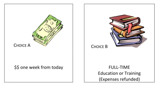
(7) allows a comparison of what the subject would do in each situation. Since the subjects know they will be paid for one of their decision, but they do not know which one before the end of the session, they have the incentive to reveal what they really want for all decisions. An example of an educational subsidy choice is pictured in Figure 2.1 below. This particular example offers a choice between a $1000 grant and $25 cash. Given that these subsidies are only available for a limited time (two years from the date of the study), if a participant has no interest in acquiring additional education, he or she will opt for the cash. The complete set of decisions presented to participants is available upon request.. Figure 2.1: Example of Educational Subsidy Choice. You must choose A or B:. CHOICE A. Decision 124. CHOICE B. $$ one week from today. FULL-TIME Education or Training (Expenses refunded).  $25.  $1000 GRANT. Four subsidy types were used in the choices provided to participants: Grants, Loans, Hybrid Loans (½ loan, ½ grant), and Income Contingent Hybrid Loans. The grants varied from $500 $4000, the loans varied from $1000 - $4000 and the Hybrids varied from $800 - $4000. Cash alternatives varied from $25 - $700. These decisions are summarized in Table 2.1..

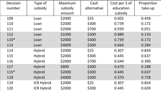
(8) To participants in the study, accepting a grant, loan or hybrid is not free. They must pay a price, which is the cost per dollar of subsidy accepted. No matter what the subsidy type is, participants have to give up a certain amount of cash. For instance, if they choose a $1000 Grant rather than a $25 cash alternative (Decision 124), their cost would be $25 /$1000 or 2.5 cents per dollar of subsidy. If they choose a loan rather than the cash alternative, they have given up the cash alternative but gotten the use of the subsidized loan for approximately 5 ½ years, interest free. If participants choose a $1000 loan rather than $300 cash alternative (Decision 112), the cost of the subsidy would roughly include the $300 they gave up to get the loan, plus the inflation depreciated payback at the end of approximately 5 ½ years, less the value of subsidized interest for approximately 5 ½ years. In other words, the cost per dollar of loan subsidy would be [Cash + PV of the loan – subsidized interest] / Subsidy amount. For decision 112, it would be [300 + (1000-141.86)-269.14]/1000 = $0.917.3. Table 2.1: Educational Finance Decisions. 3. Decision number. Type of subsidy. 109 110 111 112 110* 113 114 115 116 117 115* 118 119 120. Loan Loan Loan Loan Loan Loan Hybrid Hybrid Hybrid Hybrid Hybrid Hybrid ICR Hybrid ICR Hybrid. Maximum subsidy amount $2000 $2000 $2000 $1000 $2000 $4000 $2000 $2000 $2000 $800 $2000 $4000 $2000 $2000. Cash alternative $25 $300 $700 $300 $300 $300 $25 $300 $700 $300 $300 $300 $25 $300. Cost per $ of education subsidy 0.602 0.739 0.939 0.889 0.739 0.664 0.307 0.445 0.644 0.670 0.445 0.370 0.307 0.445. Proportion take-up 0.458 0.172 0.051 0.110 0.172 0.284 0.834 0.637 0.390 0.288 0.637 0.728 0.854 0.659. For this table and the computations presented in this report, for loans, a 2.5% inflation rate, 3% real interest rate, and 5 ½ years of interest subsidy were assumed. This is slightly different than the field implementation of a 2.5% inflation rate. This small discrepancy should have a minimal impact on the findings and no qualitative impact..

(9) Decision number. Type of subsidy. 121 122 120* 123 124 125 126 127 128 126* 129 130. ICR Hybrid ICR Hybrid ICR Hybrid ICR Hybrid Grant Grant Grant Grant Grant Grant Grant Grant. Maximum subsidy amount $2000 $800 $2000 $4000 $1000 $1000 $1000 $1000 $500 $1000 $2000 $4000. Cash alternative $700 $300 $300 $300 $25 $100 $300 $700 $300 $300 $300 $300. Cost per $ of education subsidy 0.644 0.670 0.445 0.370 0.025 0.100 0.300 0.700 0.600 0.300 0.150 0.075. Proportion take-up 0.377 0.295 0.659 0.742 0.886 0.823 0.687 0.413 0.385 0.687 0.764 0.836. *These decisions were presented only once in the study. They are repeated here to demonstrate potential groupings or comparisons of decision arrays. The cost per dollar of subsidy must overlap substantially for loans and grants in order to be able to more clearly distinguish the impact of loan aversion. For instance, if a participant favours one type of subsidy versus another when the prices of each subsidy are the same, it would indicate a preference or an aversion towards one particular type of subsidy. If subjects are willing to pick grants, but not loans that are priced the same, then this would indicate the presence of loan aversion. We recognize that presenting subjects with similar effective prices does not guarantee that they will see it that way. In the eyes of participants, the effective price of a loan is in part subjective and linked to different perceptions regarding future interest rates and inflation rates. In order words, subject may see important differences in effective prices between grants and loans when these are in fact quite similar. The experiment attempted to limit these variations in subjects’ perceptions by reminding them of current interest rates and proposing plausible inflation rate scenarios in the material provided at the session. In the end, if large differences in preferences are observed, favouring grants versus loans at comparable prices, we could then attribute these differences to loan aversion..

(10) Perhaps some of the most interesting choices are those made by students at the margin, that is, those who are somewhat motivated to attend PSE, but may also be loan averse. They may vary their willingness to invest in PSE as a function of the financing options available – for example, they may be more likely to choose grants over cash, but cash over loans. These decisions tell us how generous financial assistance needs to be in order to induce marginal participants to invest in PSE. To investigate whether some groups are less likely to borrow, after controlling for the price of educational subsidies, we relate the educational subsidy choices of participants to their vital characteristics collected from the baseline measures — socio-economic groups, numeracy level, risk and time preference, etc. The baseline measures include demographics, attitudes and behaviours, (from the subject survey); socio-economic status and attitudes (from the parental survey); a numeracy assessment (from the numeracy assessment), and measures of intertemporal and risk preferences (from the laboratory experiment). This comprehensive set of measures on resources, attitudes, behaviours, preferences and ability provides a unique opportunity to create an extremely rich data set describing the characteristics of each participant. Student Survey Obtaining a good profile of the participants and their family context was essential to this study. Many relevant and excellent survey questions were adapted from the Youth in Transition Survey (YITS), Post Secondary Education Survey (PEPS) and Survey of Labour and Income Dynamics (SLID).4 These data include measures on: educational ambitions, expectations with regards to ambitions, perceived obstacles to pursuing PSE, financial means at student’s disposal, debt aversion, and experience with debt, educational background, educational experiences, parent’s education and parent’s economic status. In addition, several other scales were included 4. These questions are available to duplicate at no charge as long as Statistics Canada is acknowledged as the source..

(11) to assess other attitudes and behaviours like inter-temporal orientation (planning ability), attitudes towards risk, aspiration level, engagement while in high school, perceptions of labour market conditions and perceptions of the cost of, and returns to, PSE. In short, we attempted to include as many as possible of the questions on personal characteristics, attitudes, or behaviours that have been shown in previous research to correlate with educational choice. Parental Survey Some of the questions asked of parents were redundant with the students survey, but provided more reliable data. Parents were interviewed by telephone for basic income information, educational background and expectations concerning their child’s educational achievement. Numeracy Assessment For many, the lack of basic literacy skills represents the most severe barrier to participation in education. Numeracy skills are often a gatekeeper for entrance into further education in many occupational areas and can critically affect employability and career options. Numeracy assessments typically involve the use of mathematics in real-life situations.5 The results of this assessment provide a rough gauge of an individual’s overall literacy competencies and allow for investigation of the relationship between the readiness to learn and the decision to invest in learning. It is also possible to make comparisons between perceived and measured ability to learn. Measurement of preferences In addition to survey measures providing a relevant set of preferences pertaining to investment behaviours, we used the experimental sessions designed to capture the willingness 5. Numerate behaviour is observed when people manage a situation or solve a problem in a real context; it involves responding to information about mathematical ideas that may be represented in a range of ways; it requires the activation of a range of enabling knowledge, behaviours and processes. See Gal (2000)..

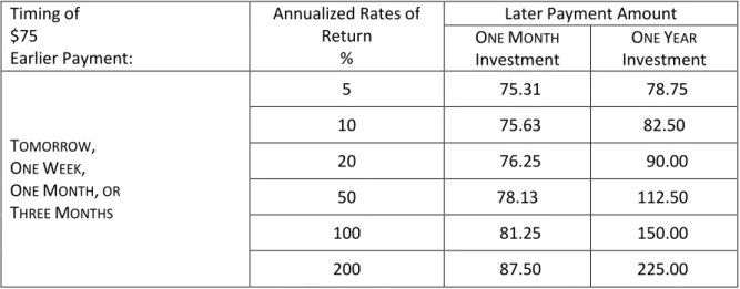
(12) to take up different offers of financial aid to also collect inter-temporal and risk preferences using experimental techniques. 1. Inter-temporal preferences In principle, time preference of an individual can be measured by offering a choice between two payments of different value to be made at different points in time. The later payment will have a greater value than the earlier payment, thereby rewarding the subject for delaying gratification, i.e. rewarding saving. The payments depend on the size of the initial endowment, the rate of return to saving, the timing of the earlier payment and the waiting time for the later payment. (Eckel, Johnson, and Montmarquette, 2002 and 2005; Harrison et al., 2002) By varying these parameters and offering each respondent a set of binary choices, one can develop a comprehensive picture of each subject’s willingness to forgo smaller returns sooner for larger returns later. The set of time preference choices is summarized below in Table 1.. Table 2.3: Summary of Time Preference Choices Timing of $75 Earlier Payment:. TOMORROW, ONE WEEK, ONE MONTH, OR THREE MONTHS. Annualized Rates of Return %. Later Payment Amount ONE MONTH ONE YEAR Investment Investment. 5. 75.31. 78.75. 10. 75.63. 82.50. 20. 76.25. 90.00. 50. 78.13. 112.50. 100. 81.25. 150.00. 200. 87.50. 225.00. The earlier payment is consistently $75, paid on the date indicated, i.e., one day, one week, one month or three months from the time of the experiment. Participants have to choose between one of these “earlier payment” dates and a later payment amount (either a one month.

(13) investment period or a one year investment period). One month and three month earlier payments are included to test and control for possible hyperbolic discounting (see the papers in Loewenstein et al., 2003).. 6. All eight decision time combinations are repeated using six. annualized rates of return, as shown in the table. A broad range of rates of return is included because our previous results have suggested a great deal of variation in subject preferences (see Eckel et al., 2005). Finally, decisions involving both short (one month) and long (one year) investment periods are included. A person’s willingness to delay payment cannot be underestimated. In each of our previous studies, experimentally measured patience has explained a fair proportion of the variation in the outcomes data: willingness to invest in own education, willingness to invest in a family member’s education and willingness to invest in long term savings. (See Eckel, Johnson, and Montmarquette, 2002; and Johnson, Montmarquette, and Eckel, 2003.) 2. Attitudes towards risk Attitudes towards risk in a population play a key role in many models of economic and social behaviour, yet they are typically treated as unobserved characteristics in empirical analyses of individual decisions. Results from risk experiments conducted on college students (Eckel and Grossman, 2002; Holt and Laury, 2002), adults in Canada (see Johnson et al., 2004), and Houston high school students indicate substantial heterogeneity in responses. In the Canadian studies, these responses correlate with important lifetime decisions, including decisions about investments in education. We used two sets of decisions under uncertainty. One set was a graphical representation of the Holt and Laury (2002) 10-binary decision instrument, scaled three different ways. The. 6. “Today” and “Tomorrow” early payoff choices are sometimes included to test for a possible confound, i.e., whether the experimenter is trusted by the subject to pay future amounts. If the subject doubts future payments, his choices will make him appear more impatient than he really is. In our earlier work with very similar instruments, we tested for trust effects by comparing results for today vs. one month and tomorrow vs. one month and find no significant difference. Thus there was no trust issue arising in our data at the time..

(14) second set was 5 graphical versions of the one out of six 50/50 gambles based on Eckel and Grossman (2008).7 An individual’s attitude towards risk is likely to vary depending on the decision-making domain (e.g., investment or insurance, health-related behaviour, social risks) and will also depend on whether the risk involves gains or losses. In the experimental component of the baseline measures, the focus was on risks related to abstract gambles, which are described as “cash payments with uncertain outcomes” to avoid any negative association with gambling. At the end of the session, if a risk decision was chosen for payment, the participant was asked to roll a fair die to determine the payoff for their chosen gamble.8 III. Implementation From October 2008 to March 2009 nearly 1250 Canadian students, mostly ranging in age from 16-18 years, participated in 75 experimental sessions. This sample was drawn from both urban and non-urban sites across Canada and was made up of full-time students, most of whom were enrolled in high school and some in CEGEP. Sample To generate meaningful comparisons by population group, the original project design called for 1400 respondents with the goal of recruiting a minimum of 200 participants per group of interest – high and low SES, aboriginals and rural vs. urban – in three or four different provinces. The 1248 teenaged students were recruited from across Canada, representing both rural and urban areas as well as low and middle income areas. Although not a focus of the stratified sampling strategy, special attention was paid to document immigrant students and students from single parent families for use in the analysis. A small number of participants over the age of 18 were included primarily because one participating high school had adult learners who had 7 8. Details are available upon request Note that the measurement of other domains of attitudes towards risk was included in the survey component of the study..

(15) returned to school. These older students represented approximately six per cent of the sample. Table 3.1 summarizes the numbers of participants in several groups of interest and by selected characteristics. Table 3.1: Participants Total Population = 1248 Male. 577. Female. 671. Rural (U > 40 km). 152. First Nations. 110. Low Income. 218. First Generation PSE. 352. Single Parent Family. 123. Work > 20 hours per week. 794. High School. 948. A sample of non-urban residents was recruited to compare their behaviours to urban residents. People in rural areas may face particular barriers to learning: transportation costs, lack of access to education providers, or simply reluctance to leave a community that they are deeply attached to. For many individuals in more remote areas the decision to pursue education may mean abandoning their social ties and a way of life that they cherish. The project design called for 400 participants from rural areas to allow meaningful analysis and comparisons between rural and urban behaviour. For the purpose of the analysis, this sample size would allow subgroups to be created that included one characteristic in addition to the rural/urban characteristic. Unfortunately, however, the recruitment efforts, summarized in the next subsection, were only able to attract 152 rural participants, defined as students whose.

(16) permanent residences were located more than 40 km away from a university, although 244 students could be classified as attending a school that met that criterion.9 Experimental Protocol The experimental sessions were held in controlled environments including classrooms, libraries, career counselling rooms, activity rooms and auditoriums. All sessions were held on the campus where the student attended classes. As the demand for different session times in different locations varied, a total of 75 sessions were conducted with 50 as the maximum number of participants in any session. For showing up on time, each participant received a $20 show-up fee. This fee guaranteed that they would not leave the experiment empty-handed and allowed the experimenters to show the participants that they keep their word in terms of making promised payments. It also helped the participant to feel committed to finishing the experiment, and, most importantly, encouraged the participants to show up on time. All participants received an identification number to protect their confidentiality. Participants were also reminded that this was a volunteer study, one that required their consent (Participant consent was obtained prior to filling out the web survey). During the introduction to the experiment, participants were told that they could earn substantially more than their showup fee by completing three parts of the study. The in-school session included the two remaining tasks: a set of real decisions about financial aid and the life skills assessment (numeracy). The experimenter provided participants with appropriate details of the compensation available. This compensation included opportunities to receive both cash rewards (in the form of a check) and non-cash rewards in the form of educational financing. All participants were provided with the following information regarding the educational financing:. 9. Only 46 participants lived 40 km away from any type of PSE institution, including CEGEP or community colleges..

(17) Grants — Educational grants will be disbursed if a participant enrols in an institution for learning or training full time within two years from the date of experiment participation. Loans — Educational loans will be disbursed if a participant enrols in an institution for learning or training full time. These loans will be available up to two years from the date of the experiment. The loans are repayable upon the completion of the study or if the participant drops out of the program of study. The interest rate floats and is set at the prime rate plus 2.5%. ICR loans — ICR educational loans were described as identical to the “loans” described above with the additional feature that repayment can be suspended, but not forgiven, if the income of the participant falls. Participants were advised that all types of support must be for direct or indirect expenses related to a program of study at an authorized institution. The financial support would only be awarded if the participant, not a family member or friend, enrolled during the two years following the experimental session. Additionally, any financial aid received through this study could not be disbursed to pay for past educational investments. To familiarize participants with the experimental decisions, 22 practice examples, one for each kind of experimental decision, were given to the participants before they began completing any of the real decisions. It was essential that they understood the nature of the decisions and how payment would be made. This practice was conducted with a lot of one-onone help. The field crew was made up of three to five people on hand to ensure that all participants got the attention they needed to complete the practice decisions and the actual choices during the experiment. In completing the actual choices, participants made a decision for each choice and, after all decisions were made, one decision was selected at random for each participant and the participant received the payoff corresponding to the choice made for the selected decision..

(18) Participants used a bingo ball cage where each decision number was matched with one corresponding numbered ping pong ball to randomly select the decision they would be paid for. Each decision had an equal probability of being selected, making decisions independent of each other. The experimental decisions were checked by the study staff while participants completed their numeracy assessments. Where necessary, participants were informed of missed decisions or illegible answers so that they could answer all decisions prior to the random selection process. This process of checking was instituted primarily to ensure that all experimental decisions were answered and to prevent the possibility of randomly selecting a decision for compensation where no choice had, in fact, been made. The overall experience for each participant was scheduled to take two hours. Some participants finished in as little as 1 hour 40 minutes, others took up to three hours to complete both parts. Although the numeracy assessment was estimated to take 30 minutes to complete, explicit instructions were provided to the experiment delivery team that participants should not be rushed to finish the assessment. In practice however, the numeracy assessment took far more than 30 minutes to complete for a majority of the participants. IV. Investigating the Demand for Educational Subsidies This section of the report takes a first look at the experimental choices made by subjects on the types of financial aid offered. We begin simply by observing the impact of the design parameters -- cost per dollar of educational subsidy and type of subsidy -- on the number of students accepting educational subsidies. Using the costs per dollar of financial subsidy derived earlier and presented in Table 2.1, we can depict demand curves for financial aid by type of subsidies. In subsequent sections, we will investigate the determinants of this demand through multi-regression analysis. For now, we limit the discussion to a mere description of the relationships between price and demand for different sub-groups and categories of subjects..

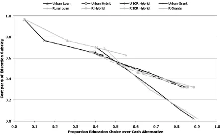
(19) Figure 4.1 depict the demand curve for financial aid resulting from the choices made by all participants to the experiment, with the proportion of respondents that chose education over a cash alternative by type of subsidy on the horizontal axis, and the cost per dollar of education subsidy, or the price of the subsidy, on the vertical axis. The set of choices presented here reflects a constant subsidy amount and allow the cash alternative to vary. For instance, starting at the left most point, 5.1 per cent of participants chose the option of a $2000 loan for PSE over a $700 cash alternative, 17.2 per cent chose a $2000 loan over a $300 cash alternative and 45.8 per cent chose a $2000 loan over a $25 cash alternative, at respective prices of $0.94, $0.74, and $0.60 per dollar of loan subsidy. The decision numbers are noted in the graph for ease of comparison with decision characteristics and reported take-up proportions found in Table 2.1.. Figure 4.1. We combine nine other decisions and four decisions used above to illustrate another demand curve over the same price range. This time instead of allowing the cash alternative to vary, Figure 4.2 used a collection of decisions where the cash alternative is kept constant at.

(20) $300, but the amount of subsidy offered vary. Figures 4.1 and 4.2 are plainly consistent with one another. Both figures show clearly that the price of the subsidy matters to participants. Both figures show downward sloping demand curves indicating that participants were mindful of the relative values of the different subsidies they were offered.. Figure 4.2. Whether or not the type of educational subsidy matters is to be investigated more thoroughly in the analysis section. But for now, we can observe that demand for grants seems to lie slightly lower than offers of very low-priced loans (hybrids). One would expect the opposite, as one would thing a priori that, for a same price, grants would be more attractive than any types of financial aid including loans. As well, the addition of a set of decisions allowing for repayment of loans to be based on the ability to repay (ICR Loan Hybrid), seems to have a negligible impact on overall demand. We now turn to representations of the demand for financial aid by sub-groups and individual characteristics to flesh out some more basic observations. Given that both.

(21) representations of the demand for financial aid are strikingly similar whether we keep the cash alternative constant (Figure 4.2) or the amount of subsidy constant (Figure 4.1), we will present the next set of descriptive results using one of these representations only. THE IMPACT BY POPULATION SUB-GROUP Figure 4.3 summarizes the demand for educational subsidies when the sample is split into rural and urban participants. The dark lines represent the demand by urban participants and the lighter gray lines represent the demand by rural participants. Urban participants are defined as those who live within 40 km of a university. There is hardly any difference in these respondents with respect to their behaviour for grants and low-priced loans (half grant/half loan). But there does seem to be a larger willingness to finance education with loans on the part of rural respondents.. Figure 4.3 Educational Subsidy Demand by Geographical Proximity to a University. Both parents and students were asked if they identified themselves as a Treaty Indian, Registered Indian or a member of an Indian Band/First Nation. If students responded yes to this question, they are identified as “First Nation” in Figure 4.4. All those that said no to this question.

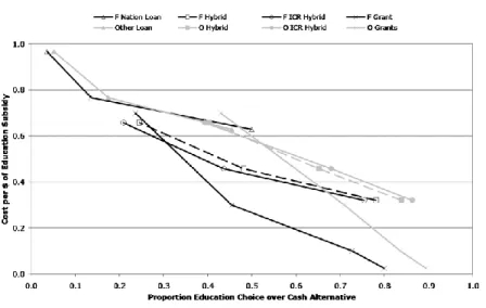
(22) are identified as “Other” and their responses are coded with light gray lines. Those who identified as First Nation have across the board noticeably lower demands for educational financing.. Figure 4.4: Educational Subsidy Demand by Identifying as First Nation. 210 or 16.8 per cent of participants came from households with no PSE experience. Figure 4.5 summarizes the demand for this population subgroup with the black lines and the subpopulation with PSE experience with the gray lines. The First Generation PSE sub-sample seems to be demanding much less education at prices less than $0.65 per dollar of educational financing as compared with their counterparts.. Figure 4.5: Educational Subsidy Demand by First in Family to go to PSE.

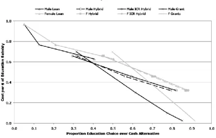
(23) Fir st Ge n e r a t ion PSE First Gen Loan. F Hybrid. F ICR Hybrid. F Grant. Other Loan. O Hybrid. O ICR Hybrid. O Grants. 1.0. Cost pe r $ of Edu ca t ion Su bsidy. 0.8. 0.6. 0.4. 0.2. 0.0 0.0. 0.1. 0.2. 0.3. 0.4. 0.5. 0.6. 0.7. 0.8. 0.9. 1.0. Pr opor t ion Edu ca t ion Ch oice ove r Ca sh Alt e r n a t ive. Many of the traditional groups usually known for lower participation in PSE show evidence of such lower participation in the simple demand curves constructed above. Students from low-income households, from households with no PSE experience, from Indian Band/First Nation populations, all exhibit, to some extent, lower willingness to invest in PSE than the general population. Students from rural areas and Immigrant families do not exhibit these tendencies. The next part of this section examines how personal characteristics interact with the decision to invest. THE IMPACT OF INDIVIDUAL CHARACTERISTICS, BEHAVIORS AND ATTITUDES This study affords a rich array of data by which to categorize participants. The next ** figures highlight some of the basic relationships found in that data, starting with basic individual differences and ending with more subtle attitudes and behaviours. Men and women respondents averaged the same response rate on one decision only – the most expensive loan. They tie at approximately five per cent of the population choosing the.

(24) $2000 loan over the $700 cash alternative. (Upper left point on Figure 4.6.) At every other price, women express a much higher demand for student aid, and indirectly for PSE, than their male counterparts.. Figure 4.6: Educational Subsidy Demand by Gender. All participants completed a numeracy assessment. As a reminder, numeracy is a combination of ability and skill level, not an intelligence test. Numeracy can be learned. The numeracy assessment was normalized to the Canadian population and each participant was awarded a score between 0 and 500. This score was used in the regressions that will be discussed in the next sections. For a cursory look at the relationship between the demand for education and a subject’s numeracy skills, we subdivided the population into four groups: 0-200, 200-300, 300-400 and 400-500. Over ninety per cent of the participants fall into the two middle categories. Participants with a score over 300 can be thought of as PSE ready..

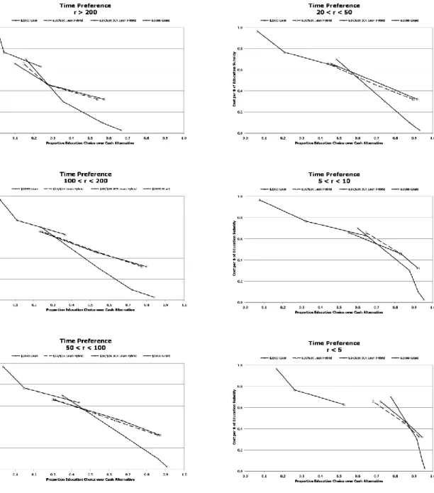
(25) Figure 4.7: Educational Subsidy Demand by Numerate Skill Level. Clearly, as numeracy increases, so is the demand for financial aid to pursue PSE. The positive relationship between numerate ability and willingness to pursue PSE is only dwarfed by the relationship between willingness to save and willingness to pursue PSE (Figure 4.7). The title on each graph in Figure 4.7 roughly indicates the interest rate at which the participants could be induced to save for one year. The graphs are presented in order of increasing patience with the last graph summarizing the behaviour of the close to six per cent of the population that saved at every option. Participants willing to save and to postpone instant gratification are clearly inclined to express a much higher demand for PSE financing and studies..

(26) Figure 4.7: Educational Subsidy Demand by Student’s Willingness to Save for the Future.

(27) The study included several possible measures of attitude towards risk. We found a subtle and positive correlation between risk aversion and demand for PSE, but none of those relationships merited a graphical representation here. We include a measure for risk in the multivariate analysis used in the next sections to see if the relationship holds. The next figure focuses specifically on student behaviour while in high school: grades. The positive relationship between grades and the demand for PSE is striking but not surprising. In Figure 4.8, the demand curves seem to walk across the page as we move from low grades, to medium grades and to high grades.. Figure 4.8: Educational Subsidy Demand by Student’s High School Grades.

(28) The next two figures summarize some of the most dramatic relationships between expectations and the demand for PSE financing. Approximately five per cent of the students in our sample expect to drop out of high school. This expectation manifests itself in a dramatically lower demand for PSE financing.. Figure 4.9: Educational Subsidy Demand by Student’s Expectation to Dropout. Empirically, there is little correlation between parent expectations and outcomes in investment in PSE by children. For this reason, we investigate the student’s perception of family expectations. Indeed, in our sample, nearly all parents surveyed, 92 per cent, expect their child.

(29) to go on to PSE but only 78 per cent of students believed their family expected them to go on to PSE. When the sample is partitioned with respect to students’ beliefs regarding their family expectations, there is a striking separation of behaviour. The dark line segments in Figure 4.10 represent the choices of those students who think their parents expect them to go to PSE. Nowhere do the two demand curves cross. Figure 4.10: Educational Subsidy Demand by Family Expectations (Student Survey). The final figure shows the relationship between experience with saving and demand for PSE financing. Students were simply asked if they had ever saved any money for PSE. Those that claimed to have saved any money for PSE show a marked increase in the willingness to accept educational financing of all types..

(30) Figure 4.11: Educational Subsidy Demand by Personal Savings and No Savings for PSE. The above figures show that many factors singularly influence the demand for education. What is very clear through the 12 figures is that every partition of the sample whether it is by subgroup, individual characteristics, behaviour, perceptions or attitudes, gives us a downward sloping demand for educational financing. This shows that the price of education is clearly a principle consideration in the willingness to participate in PSE. In the next section, we jointly analyze simultaneously the many potential factors, in addition to price, that influence the demand for PSE financing. V. Overall Demand for Educational Subsidies: What Matters? In this section, we use a regression framework to address what matters in the demand for student financial aid and to assess, in particular, the role played by different types of aid. We first divide the participants in two distinct groups: those who never chose an educational subsidy, and those who show much interest by choosing educational subsides over cash in almost all decisions. After analyzing the characteristics of these two groups, we analyse what.

(31) matters in the demand for educational subsidies for all participants. In Section 6, we tackle the question as to whether there is any systematic behaviour representing loan aversion among our subjects. Who is interested in PSE? Some 9 per cent of participants (113) never chose an educational subsidy offer. Even when such subsidy cost them as low as 2.5 cents per dollar of aid, these participants preferred cash. At the other spectrum, there are about 7% of participants (73) who chose education over cash offers either every time or almost every time (at least 21 times out of 22 opportunities). We use two probit models to investigate those who are either out of the market for PSE financing (NEVER) and those that take education consistently at least 21 times out of 22 ( ALWAYS). Table 5.1 reports the results. Note that for each model, we present two specifications. Specification 1 considers group variables only. Specification 2 adds individual characteristics, attitudes and behaviour variables. Table 5.1: Preference for Educational Subsidies NEVER PSE Québec. ALWAYS PSE. -0.0402 -0.18. -0.03 -0.109. 0.00109 0.00442. -0.027 -0.0956. Manitoba. 0.499*** 2.919. 0.684*** 3.306. 0.00684 0.0361. -0.0538 -0.254. Saskatchewan. 0.955*** 3.781. 0.849*** 2.836. -0.913** -1.998. -0.935* -1.764. Rural (Univ > 40 km). 0.285 1.568. 0.318 1.488. 0.215 1.109. 0.272 1.248. First Nation. 0.134 0.777. -0.0635 -0.312. -0.191 -0.789. -0.129 -0.464. Single Parent. 0.218 1.295. 0.304 1.558. 0.0245 0.118. -0.111 -0.479. Missing Value Single Parent. 0.253 0.919. 0.329 1.019. 0.158 0.483. -0.00819 -0.0223. First generation PSE. 0.210* 1.797. 0.0182 0.131. 0.169 1.269. 0.304** 2.025. Immigrant. -0.244 -1.031. -0.228 -0.791. 0.385* 1.726. 0.468* 1.885.

(32) Low Income (< 40K). -0.112 -0.705. -0.371 -0.925. -0.134 -0.744. 0.00258 0.00526. Missing value Low Income. -0.102 -0.383. -0.5 -1.583. -0.351 -1.062. -0.114 -0.309. Low Inc Montreal (renters). 0.336 0.75. 0.456 0.879. -0.0854 -0.161. -0.196 -0.315. CEGEP. 0.0933 0.395. 0.25 0.883. -0.233 -0.87. -0.259 -0.818. -0.729** -2.228. -0.525 -1.345. 1.171** 2.353. 1.291** 2.232. 0.0632 0.396. -0.0373 -0.2. -0.0474 -0.252. -0.0396 -0.188. Adult Student Volunteer outside of class Female. -0.175 -1.368. 0.2 1.39. Numeracy. -0.0019 -1.641. -0.000947 -0.743. Willingness to Save. -0.262*** -5.568. 0.143*** 3.348. Risk Seeking. -0.129*** -3.249. 0.0524 1.201. Risk Seeking X Low Income (< 40K). 0.0418 0.452. -0.0235 -0.227. Grades 60 - 80. -0.379* -1.785. -0.295 -0.71. Grades > 80. -0.745*** -2.911. -0.0313 -0.0733. Family expectation: Univ.. -0.452*** -3.462. 0.695*** 2.917. Peers not go to university. -0.0807 -0.603. 0.00251 0.0154. Obstacles to prevent PSE. 0.0322 0.241. 0.128 0.87. Possibility drop out of HS. 0.399 1.6. 0.0849 0.202. Skip Class (> once month). -0.169 -1.174. -0.165 -1.005. Works > 20 hrs per week. 0.274** 1.972. -0.299** -2.23. 0.0138 0.104. -0.123 -0.79. -0.0145*** -3.341. 0.00946** 1.963. -0.0812 -0.371. -0.43 -1.577. 0.241 1.491. -0.00755 -0.0399. Hesitant to undertake a university education b/c of the amount of debt Organisation and planning Owns Credit Cards Personal level of debt to be a burden.

(33) Family’s level of debt to be a burden Personal Savings for PSE Constant Pseudo R2 Observations. 0.0513 0.342. 0.433*** 2.783. -0.275** -2.076. 0.227 1.617. -1.804*** -8.865. 1.963*** 2.927. -1.516*** -6.733. -3.491*** -4.201. 0.0664. 0.2791. 0.0346. 0.1808. 1248. 1248. 1248. 1248. t-statistics presented below coefficient estimates. ***: significant at 1%; ** significant at 5%: * significant at 10%. Two tail tests. The first model of Table 5.1 studies the determinants of those who never took a single educational subsidy. The observed corresponding variable to the latent (unobserved) “no preference for education” is 1 if the participant has refused all educational subsidy choices, that is always choosing the cash alternative for all the 22 choices, and zero otherwise. The Pseudo-R2 for both specifications, a measure of goodness of fit of the model, shows that the inclusion of individual variables is needed to obtain a relatively good fit. Therefore, we will only comment on the results of Specification 2 for the first model. Results show that there is a greater probability of a participant from Manitoba and Saskatchewan relative to participants from Québec and Ontario to show no preference for education. Similarly, students who work at least 20 hours per week in the labour market have a greater probability of never investing compared with their less labour market engaged peers. However, there is a long list of characteristics and behaviours that reduce the probability to never choose educational financing. Two exhibited behaviours include a WILLINGNESS TO SAVE ($75 for a year at various interest rates) and a willingness to take on more risk than their peers (RISK SEEKING). Additionally, those with high grades (averages above 80), high family expectations regarding their success at University, a good sense of organisation and planning, and personal savings for PSE all had a lower probability to never choose education. The second model moves our focus to the other end of the spectrum seeking to characterise those participants who consistently choose the educational subsidies alternatives over cash. In this probit model, the dependent variable is 1 if the participant has chosen at least 21 out of 22.

(34) educational subsidies and 0 otherwise. As before, the specification including individual characteristics yields a reasonably good fit. Five important individual factors increase the probability of being in the group of participants who consistently choose educational subsidies over cash: First Generation PSE. Adult students, immigrants, relatively more patient participants (WILLINGNESS TO SAVE), students who are encouraged by their family to obtain a university education and students who consider the family’s level of debt to be a burden. But students from Saskatchewan, relative to other provinces, and students who declare working 20 hours or more while in school relative to those less engaged in the labour market are less likely to be among the group of individuals showing very strong preference for educational subsidies. The demand for educational subsidies: what matters? We now examine the participants’ willingness to take up educational financing controlling for the different subsidy forms, for prices of these financial instruments, group variables and individual and socioeconomic characteristics of the participants. The demand for educational subsidies is estimated within the context of a linear probability model. The pooling of the individuals choosing among 22 choices of educational financing vs. cash alternatives creates the opportunity to report an individual effect with GLS estimates. With 1248 individuals and 22 decisions, the total amount of observations available to conduct estimations is 27.456. The coefficients can be interpreted directly as marginal probabilities since this is a linear probability model. Specification 1 of Table 5.2 uses only the price variable in addition to the usual constant. The regression coefficient on price is negative and highly significant. The demand for educational subsidies, or the willingness to give up a cash alternative in favour of student aid, increases as the price of the subsidies decreases. Given how parsimonious the specification is, the overall R2 of 0.2465 indicates a nice fit..

(35) Specification 2 adds the subsidy type -- Grants, Loans, Hybrid -- with the Income Contingent Loan hybrid as the reference. The three added subsidy type variables do not significantly increase the overall goodness of fit of the model (R2 = 0.2557) relative to the first specification. In other words, relative to price, the subsidy types do not explain very much of the demand for educational financing. With Specification 3, we assume that the subsidy types not only affect the intercepts of the demand curve, but also the slope.10 Through these two effects (Subsidy and Price x Subsidy), we can see that a grant subsidy generates more demand than loans only when the price per dollar of subsidy is above 42 cents.11 The price per dollar of funding must reach a relatively high level before a significant difference on the demand for educational financing occurs between the two forms of subsidy in favour of grants. Compare to Specification 1, the overall R2 increases by 8.7 per cent, reaching 0.2680. Table 5.2: The demand for educational subsidies Model 1 Model 2 Price Grant. -0.973*** -121.5. Model 3. Model 4. Model 5. -0.986*** -89.06. -1.469*** -51.29. -1.491*** -51.59. -1.425*** -43.02. -0.106*** -17.59. -0.406*** -26.18. -0.406*** -26.2. -0.406*** -26.31. 0.715*** 22.38. 0.715*** 22.4. 0.715*** 22.5. -0.282*** -9.714. -0.282*** -9.724. -0.282*** -9.765. 0.420*** 9.729. 0.420*** 9.74. 0.552*** 12.53. -0.0418** -2.031. -0.0418** -2.033. -0.0418** -2.042. 0.0651 1.608. 0.0651 1.61. 0.0651 1.617. -0.0411 -1.286. -0.0375 -1.357. Price x Grant Loan. -0.0951*** -14.12. Price x Loan Hybrid Price x Hybrid Québec. 10. -0.0101* -1.687. There is practically no difference in behavior between the hybrid loan and an ICL-hybrid loan, the reference variable. 11 The differential effect on the demand for education between a grant and a loan is: (-0.406 + 0.715 x Price of $1 funding) - (-0.282 + 0.420 x Price of $1 funding). The differential is positive if Price is greater than 42 cents per dollar of educational financing..

(36) Manitoba. -0.0709*** -2.75. -0.0755*** -3.516. Saskatchewan. -0.317*** -7.305. -0.237*** -6.394. Price x Saskatchewan. 0.163*** 6.86. 0.134*** 5.558. Rural (Univ > 40 km). -0.0143 -0.517. -0.0115 -0.497. -0.112*** -3.562. -0.0559** -2.045. Price x First Nation. 0.0506* 1.801. 0.0329 1.171. Single Parent. -0.0291 -1.073. -0.0420* -1.866. Missing Value Single Parent. 0.0134 0.324. 0.00629 0.183. First generation PSE. -0.0391** -2.171. -0.00401 -0.266. Immigrant. 0.120*** 3.293. 0.117*** 3.685. Price x Immigrant. -0.0634** -1.975. -0.0731** -2.27. Low Income (< 40K). -0.0153 -0.65. -0.0385 -0.828. Missing value Low Income. -0.0275 -0.698. 0.0304 0.927. Low Inc Montreal (renters). -0.0128 -0.199. -0.00815 -0.152. CEGEP. -0.00782 -0.234. -0.0288 -0.994. Adult Student. 0.203*** 3.783. 0.134*** 2.995. -0.0221 -0.859. -0.0147 -0.69. First Nation. Volunteer outside of class Female. 0.0558*** 4.126. Numeracy. 0.000202 1.625. Willingness to Save. 0.0631*** 14.63. Price x Willingness to Save x Loan. -0.0523*** -13.9. Risk Seeking. 0.00974** 2.36. Risk Seeking X Low Income (< 40K). 0.0105 1.055.

(37) Grades 60 - 80. -0.0142 -0.45. Grades > 80. 0.0607* 1.779. Family expectation: Univ.. 0.124*** 6.893. Price x Family expectation. -0.0743*** -4.082. Peers not go to university. 0.00918 0.618. Obstacles to prevent PSE. -0.0016 -0.114. Possibility drop out of HS. -0.0548 -1.626. Skip Class (> once month). -0.0317* -1.868. Price x Skip Class. 0.00424 0.258. Works > 20 hrs per week. -0.0413*** -3.009. Hesitant to undertake a university education b/c of the amount of debt. 0.00742 0.443. Price x Debt (Hesitant…). -0.0186 -1.109. Organisation and planning. 0.00255*** 5.576. Owns Credit Cards. 0.0164 0.759. Personal level of debt to be a burden. -0.0381** -2.022. Family’s level of debt to be a burden. 0.0307* 1.887. Personal Savings for PSE Constant. 0.0482*** 3.556 1.002*** 113.3. 1.066*** 103.5. 1.301*** 78.98. 1.406*** 41.6. 0.738*** 9.793. Rho. 0.3921. 0.3976. 0.405. 0.3906. 0.2971. Overall R-sq. 0.2465. 0.2557. 0.268. 0.2904. 0.3923. Observations. 27456. 27456. 27456. 27456. 27456. Number of students. 1248. 1248. 1248. 1248. 1248. t-statistics presented below coefficients. ***: significant at 1%; ** significant at 5%: * significant at 10%. Two tail tests..

(38) With Specification 4, group variables are added to the subsidy variables of Specification 3. There is little impact on the coefficients of the subsidy and price variables, meaning that the specification is robust. Participants from Manitoba and in particular Saskatchewan demand less educational financing than participants from other provinces. FIRST NATION participants reveal a lower demand for educational financing. This is also the case for First Generation students. Adult students and immigrant demand more educational financing than their counterparts. However, these 18 group variables add little to the goodness of fit measure with a new R 2 of 0.2994 (compared with 0.2680 for Specification 3). The overall R2 increases substantially to 0.3923 with Specification 5. We add over 20 individual characteristics to the variables used in Specification 4. Again, the results on the subsidy and price variables remain robust. Among the group variables, participants from Manitoba and Saskatchewan and the FIRST NATION subgroup invest less in educational subsidies relatively to others while immigrants and older student invest more. Female students invest more than males. A key variable in terms of effect and statistical importance is the willingness to save: more patient participants invest significantly more in education. Also risk seeking students invest more in education. Showing a good sense of organisation and planning, already saving for one’s education increases the probability of investing in educational subsidies. Participants working 20 hours or more while in school invest less in education relatively to those less engaged in the labour market. Feeling that the level of debt is a burden negatively affects the demand for education. Some cross variables between subsidy characteristics and individual characteristics were included in Specification 5. The negative coefficient estimate of the cross-variable PRICE X WILLINGNESS TO SAVE X LOAN indicates that when a loan is involved, less patient participants react less to a price increase than more patient students. The less patient participants discount more.

(39) the future repayment of the loan than their more patient counterparts. We note the negative coefficient estimate in the cross variable PRICE X FAMILY EXPECTATION. In the results presented thus far, there is little evidence that debt aversion exists. The different categories of subsidies have little effect on the demand for educational subsidies. The only significant variable leading in that direction is the ¨feeling that the personal level of debt is a burden¨ while the variable ¨hesitant to undertake a university education because of the amount of debt¨ and few related others are insignificant. The next section further examines the presence of systematic debt averse individuals in the sample. VI. Loan aversion We noted in the previous section that once the price of the educational subsidy is accounted for, demand for student financial aid is not much affected by the type of aid, and the family level of debt actually influence financial aid take-up positively, the opposite of debt aversion. Participants were asked if their personal level of debt was a burden. This variable was found, however, significant in the complete specification of the model with all the other factors taken into account. Indeed, in the descriptive statistics, this variable seemed to split the sample with lower demand for those who felt such a burden, especially at low prices. In this section, we attempt to isolate a sub sample of the participants that seem to behave in a particularly loan averse way. By design, a participant who always chose a grant and never a loan is insensitive to prices and completely sensitive to subsidy type. This behaviour appears consistent with a truly loan averse participant: the participant clearly cares for PSE since grants are always accepted over cash, but he or she has no willingness to borrow to meet the same aim. Among the 1248 participants in our study, 152 or 12.2% of them made exactly that choice. For ease of discussion, let’s call this sub sample “strictly grant seeking.” Who are these participants?.

(40) We use a probit regression where the dependent variable is 1 if the participant always chooses grants but never a loan and 0 otherwise. The results are presented in Table 6.1. Specification 1 considers group variables only. Specification 2 adds individual variables to Specification 1. The Pseudo-R2 for both specifications shows that the inclusion of individual variables is needed to obtain a relatively good fit. Therefore, we will only comment on the results of Specification 2. Table 6.1: The probability of choosing always grant and never loan Model 1 Variable Group variables. Model 2 + Individual char.. Québec. 0.0414 0.208. 0.0967 0.442. Manitoba. 0.0898 0.606. 0.0789 0.497. Saskatchewan. -0.303 -1.087. -0.159 -0.532. Rural (Univ > 40 km). -0.239 -1.338. -0.226 -1.195. -0.497** -2.223. -0.405* -1.744. Single Parent. -0.196 -1.07. -0.178 -0.913. Missing Value Single Parent. -0.233 -0.926. -0.277 -1.025. -0.318*** -2.671. -0.254** -1.987. Immigrant. -0.0339 -0.163. -0.0409 -0.189. Low Income (< 40K). -0.083 -0.54. 0.011 0.0281. Missing value Low Income. 0.215 0.936. 0.308 1.224. Low Inc Montreal (renters). -0.918* -1.79. -0.918* -1.677. CEGEP. -0.117 -0.557. -0.2 -0.86. Adult Student. -0.077 -0.195. -0.317 -0.72. Volunteer outside of class. 0.156 1.032. 0.214 1.331. First Nation. First generation PSE. Female. 0.155 1.453.

(41) Numeracy. -0.000206 -0.211. Willingness to Save. 0.0754** 2.351. Risk Seeking. -0.0178 -0.555. Risk Seeking X Low Income (< 40K). 0.00896 0.106. Grades 60 - 80. -0.134 -0.435. Grades > 80. 0.227 0.71. Family expectation: Univ.. 0.418*** 2.898. Peers not go to university. 0.0654 0.542. Obstacles to prevent PSE. -0.0681 -0.63. Possibility drop out of HS. -0.750* -1.649. Skip Class (> once month). -0.109 -0.907. Works > 20 hrs per week. 0.0953 0.906. Hesitant to undertake a university education b/c of the amount of debt. -0.0837 -0.699. Organisation and planning. 0.000134 0.0375. Owns Credit Cards. 0.265* 1.694. Personal level of debt to be a burden. -0.0706 -0.435. Family’s level of debt to be a burden. -0.205 -1.506. Personal Savings for PSE Constant Pseudo R2 Observations. 0.282*** 2.689 -1.096*** -6.171. -1.842*** -3.06. 0.0386. 0.1212. 1248. 1248. t-statistics presented below coefficient estimates. ***: significant at 1%; ** significant at 5%: * significant at 10%. Two tail tests. The probability of being STRICTLY GRANT SEEKING (jointly always accepting a grant and never a loan) is lower for first generation PSE participants. It is also lower for a FIRST NATION person, for a.

(42) low income participant from Montréal and for the high school student considering the probability to drop out. The probability is higher for those students who are patient (WILLINGNESS TO SAVE),. benefit from the support of the family (FAMILY EXPECTATION: UNIV), have already saved. for the post secondary education and own credits cards. These results can hardly support the idea that student loans keep at-risk students from investing in education. If the probability of being STRICTLY GRANT SEEKING were higher for FIRST NATION participants, those from a low income or a first generation PSE family and who expect to drop out then there would be reason to believe in the presence of debt aversion. As it is, these four at-risk groups are less likely to be categorized as STRICTLY GRANT SEEKING. The positive coefficients estimates of the other variables are also puzzling. All these variables, Willingness to Save, Family Expectation: Univ, Personal savings for PSE, are showing a consistent positive effect on the probability of being STRICTLY GRANT SEEKING. One potential explanation is that for some participants a loan is not needed to pursue PSE, but a grant, no matter the price, is always welcome. This could be the case of participants who can rely on other sources of financing than student financial aid to pursue PSE, such as parent’s income. Owning credit cards and choosing all grants but never a loan is hardly consistent with loan aversion either as it is difficult to explain why a person would be averse to debt for educational investment but not for generalized debt. However this credit card result is consistent with Prelec and Loewenstein’s (1998) prediction of debt aversion in situations of planned (student loans) and unplanned debt (credit cards). Basically, they predict using the assumptions of prospective accounting and coupling that individuals will take on debt in emergency like situations (credit cards) but when they think about taking on debt, even for investment purposes, the thought of paying the loan back after consumption (investment) has occurred will cause people to take on planned debt less often..

(43) Loan averse or lower preference for education? They are only 40 participants (3.21%) choosing always the cash option when the alternative has a loan component but taking at least a grant choice. We have potentially loan averse people with heterogeneous and weaker preferences for education than the subgroup discussed above12. Table 6.2: The probability of choosing at least a grant but never a loan component Model 1 Model 2 Group variables + Individuals char. Québec Manitoba Saskatchewan Rural (Univ > 40 km) First Nation Single Parent Missing Value Single Parent First generation PSE Immigrant Low Income (< 40K) Missing value Low Income Low Inc Montreal (renters) CEGEP Adult Student Volunteer outside of class. 12. -0.0722. -0.134. -0.207. -0.322. 0.368. 0.452*. 1.541. 1.695. 1.076***. 1.222***. 3.045. 3.00. -0.0754. 0.0107. -0.241. 0.0295. -0.435. -0.705*. -1.363. -1.93. -0.134. -0.00823. -0.487. -0.0284. -0.179. -0.239. -0.459. -0.529. 0.133. 0.134. 0.819. 0.741. -0.149. -0.329. -0.45. -0.844. -0.165. 1.280**. -0.669. 2.208. -0.074. -0.144. -0.203. -0.348. 0.374. 0.216. 0.617. 0.31. 0.332. 0.593. 0.955. 1.421. -0.326. -0.0701. -0.762. -0.142. 0.275. 0.426. 1.107. 1.514. In the following probit regressions, the dependent variable is equal to 1 if the participant has always taken the cash for all choices with a loan component (D109-123) and took a grant at least one time (D124D130); 0 otherwise..

(44) Female. -0.0603. Numeracy. -0.00208. Willingness to Save. -0.211***. -0.353 -1.37 -3.623 Risk Seeking. 0.0589 1.158. Risk Seeking X Low Income (< 40K). -0.378** -2.216. Grades 60 - 80. 0.4 1.027. Grades > 80. 0.762* 1.799. Family expectation: Univ.. -0.0947 -0.514. Peers not go to university. -0.129 -0.661. Obstacles to prevent PSE. 0.174 0.984. Possibility drop out of HS. 0.136 0.34. Skip Class (> once month). 0.0931 0.499. Works > 20 hrs per week. -0.0176 -0.1. Hesitant to undertake a university education b/c of the amount of debt. -0.259 -1.342. Organisation and planning. -0.00487 -0.814. Owns Credit Cards. -0.474 -1.343. Personal level of debt to be a burden. -0.03. Family’s level of debt to be a burden. -0.485*. Personal Savings for PSE. -0.338*. -0.124 -1.871 -1.844 Constant Pseudo R2 Observations. -2.309***. -1.433. -7.658. -1.54. 0.0618. 0.1856. 1248. 1248. t-statistics presented below coefficient estimates. ***: significant at 1%; ** significant at 5%: * significant at 10%. Two tail tests..

(45) The results show two strong group variables at play: students from Saskatchewan and from low income household are likely to be member of this subgroup. However, for low income participants the probability of being part of this group decreases when they are risk seeking. Participants with a willingness to save are less likely to refuse a subsidy with a loan component but choosing at least one grant offer. In light of those results it is more the case that these people have express lower preference for education than they are loan averse. VII. Discussion Price emerges as the key determinant in the demand for educational subsidies, with the different forms of subsidies little explanatory power. At the group level, being an immigrant is a particularly important factor to positively influence the demand for educational subsidies, while being from a First Nation family depresses this demand. Among individual characteristics, participants showing patience (WILLINGNESS TO SAVE) is the key factor to predict who is likely to invest in educational subsidies. Investing requires patience. There is some practiced anticipation before reaping the reward of the investment. Family expectations, risk seeking students and good grades were also the factors that characterize the participants showing a positive preference for educational finance. What happened to our measures of NUMERACY? Why did they not enter into the regressions models in a convincing way? In fact, numeracy is correlated with many variables. Most importantly, NUMERACY is positively correlated with WILLINGNESS TO SAVE and good grades. NUMERACY and having a member of the immediate family attend PSE (complement to FIRST GEN PSE) correlate. NUMERACY and PERSONAL SAVINGS FOR PSE correlate. And those in the FIRST NATION.

(46) subgroup had no representation on the high end of the NUMERACY score.13 The relationship between WILLINGNESS TO SAVE and NUMERACY deserves further attention. All and all, our findings do not support the idea that loan aversion is a barrier for particular subgroups, especially at risk groups represented in our sample. The key finding of this study is: Price matters. Since the price matters so much in explaining the demand for educational subsidies, it suggests an obvious policy tool to attract more students in PSE. The answer is a simple one: decrease the cost of accepting educational subsidies. Loans can be further subsidized as we did in this study by pairing them with grants. Larger loans are more heavily subsidized than small loans. Loans could be in part forgiven. More grants could be given to aspiring students and graduates. Any of these suggestions would lower the cost of educational subsidies to the receiver, but not to the donor. A complementary line of policy instruments to “lowering the price” could be to bolster the “willingness to pay” for education. A slew of policies already in place works towards this aim. Correcting misperceptions about returns to education in general, pointing to the stability of employment with a tertiary degree, and the increase in opportunities available to university graduates are all included in PSE promotional materials. The benefits to university education are found across the board, for young and old learners as well as for all racial and ethnic groups. An individual characteristic that increases the willingness to pay for education is an individual’s willingness to invest in general. What developmental factors encourage good savings behaviour in general? Does attaining good numeracy skills as an adolescent increase the likelihood of good investment behaviour as an adult? There has not been enough research in this area to establish a causal connection. 13. In our sample 72% of our participants declared that one of their parents had postsecondary education and among those scoring greater than 400 on the numeracy assessment, 87% have at least a parent with PSE. 80% of those scoring 400+ on the numeracy test recognize the support of their parents for a university education while they represent 74% of the total sample. 45.67% of participants declared saving for their education and they are represented at 53.33% in the 400+ numeracy group..