On the uniqueness of local minima for general abstract nonlinear least-squares problems

This content has been downloaded from IOPscience. Please scroll down to see the full text.

Download details:

IP Address: 194.214.160.92

This content was downloaded on 01/10/2014 at 14:56

Please note that terms and conditions apply.

On the uniqueness of local minima for general abstract nonlinear least-squares problems

View the table of contents for this issue, or go to the journal homepage for more 1988 Inverse Problems 4 417

(http://iopscience.iop.org/0266-5611/4/2/007)

Iiivcr\c Prohleins 4 ( I W S ) 417-433. Printed iii the U K

On the uniqueness

of local minima for general abstract

nonlinear least-squares problems

Guy Chavent

C E R E M A D E . UiiivcrsitC. Pai-i\-Datiphinc., 75775 Paris Ccclcx 16. France

and

I n s t i t ti te N atioiia I ilc Recherche c11 I ii I o r i i i i i t iq tic e t en Au toiii'it iquc

.

Doniai i i c (IC

Volucc;iu. liocqiiencourl. 13P 105. 7S1.53 1-c C'hc\iic) Ceilcx. Fr'iiicc

Recciccd I ? June 1987

Abstract. T h e effectivctiess o l the inversion o l ii inapping q) dcliiicd oil ; I set C I?!

iioiilineiir Icast-square\ techniques relies o n . aiiiong other things, the uniqtieness o f Iociil

171 i n i in ii o I t h e le >is t - s q u ii res cri te ri 011

.

which e n s u re\ t h ;I t 11 unie r i cii I opt i m isat i o 11 ii Igor i t h m

w i l l ( i l they do) converge t o w i r d the global ininiinuin of the least-squares lunctional. We define ii number ;' depending only o n C and Q which. i f the size 01 p(C) is not too large w i t h rcspcct t o ita eurviiture. w i l l be strictly positive. thus yielding the uniqueness o l a11 Ioc;il iiiiiiiina having ii value smallcr than ;'. The condition y > O will require neither convexity ol C n o r any monotonic property o f p . h u t involves the computation o f an i n l i m u m over iK x ?IC o f l i t s t ancl second deri\atives o f Q. Numerical application to the estimation o f t w o parameters i n ii parabolic equ2ition w i l l b e given.

1 . Introduction

CO n s i d e r

E = normed vector space (norm

11 11,

) F = pre-Hilbert space (scalar product ( , )k)

C = closed, C'-path-connected subset of E p = C'-mapping of C into F

z E F a given point and the optimisation problem

find i E C such that J ( i ) s . l ( x ) V x E C where vx E C,

J(x)

= Il$(-u) - zii;.

Problem ( 1 . 1 ) is the general least-squares setting of the problem

find ,f E C such that @(i) =

z.

_(1.3)

when the right-hand side

z

does not necessarily belong t o the image set $(C). problem (1.1) cannot admit two distinct local minima

(and hence has at most one solution), provided that the distance O u r goal is to find conditions on C and $ such that

from z to @(C) is taken smaller than a certain number 7 > 0. _(1.4) 0266-561 1/88/020417+ 17 $02.50

0

I988 1OP Publishing Ltd 317

In this paper we will be able to ensure the uniqueness only of the local minima of] having a value smaller than y (propositions 3 and 4). We also seek conditions ensuring uniqueness of all local minima.

Let us now explain our motivations.

The first quesfiotz: what kind of applications have motivated the author to

undertake this study'? The answer is: parameter estimation problems. In this appli- cation,

x

is the parameter. C is the set of admissible parameters, z is the observed data and q5 is the parameter+output mapping resulting from the resolution of the model state equations and the observation operator. O u r concern is primarily with overspeci- tied inverse problems, where dim F b dim E. so that we can expect that the derivative @'(,Y) to be more o r less injective from E into F. In order to be more specific, we can give an example.

E,uanzple 1 . We consider the I D parabolic equation

r 1 ( 0 . t ) = U( I , f ) = 0 Vf

>

0

u(y. 0) = L&) Vy E [O. I ] (1.5)

when the parameters u E R'..: and b E R - have to be estimated from the measurement

z E L'(0, T ) of the solution 11 at point y = against time. Here we have x = ( a , b ) E

W'=

E , C is a given closed subset of

R'+

x R'. which represents the a priori knowledge of

the experimenter about the parameter x = ( a , b ) . and @ is the mapping which makes the t-+ U(!, t ) function of L'(0, T ) = F correspond to a given

x

= ( U , b ) E C. In this example the evaluation of @ ( x ) involves the resolution of the parabolic equation (1.5): the problem is obviously overspecified as dim F =

+

a >dim E = 21

The second quesfiotz: why d o we address the problem of uniqueness of local

minima'? T h e only way o f actually solving the parameter estimation problems described above is to undertake the minimisation of J over C on a computer. However, optimisation algorithms are only able to find local minima over a closed set. Hence the least-squares problem ( 1 . 1 ) will be practically solvable by an optiniisation algorithm as soon as C is closed and d has a t most one local minimum over C.

This w i l l ensure that the optimisation algorithm, once converged, will give the sought global minimum of]. O n e can also remark that the uniqueness of local minima implies (but is not equivalent to) the uniqueness of the solution i of problem (1. I ) , o r in terms of parameter estimation problems, the identifiability o f i from the knowledge of z a n d C. Of course, o n e other extremely important practical problem is that of the stability of the solution .i- of (1.1) with respect to perturbations of the data z : this

problem will n o t be addressed a s such in this paper, but one can remark that, when C is compact. the above uniqueness property will ensure the existence of a unique ,i- depending continuously on z as long as the distance of z to @ ( C ) is taken small

enough.

The third (Litid lust) qurstioti: what kind of conditions on C and @ are we looking for? The first idea is that we want data-independant conditions: for a given set C and mapping

4.

we want to be able to decide whether property (1.4) holds or not. If it holds we will get as a by-product the upper limit y>O t o the distance of z from @(C)

On the iiniqiieiie.ss of local minima 419 for which the uniqueness property of local minima holds. If it does not hold the experimenter will then have to acquire more data ( i . e . change the mapping

4)

and/or augment the fi priori available information (i.e. diminish the size of C ) before

checking again for property (1.4). The second idea is that such conditions will in no

way be cheap! As in view o f the applications, no hypothesis will be made o n the shape of C and

4

( n o convexity, no monotonicity), the conditions will necessarily involve exploration all over C-which of course will require a lot of computer time as soon as the dimension of C , i.e. the number of unknown parameters, increases.

Nevertheless, we believe that such a condition will be practically useful f o r problems with few unknown parameters, and that it will at least help to understand what happens in nonlinear least-squares problems. As a test for the forthcoming suf- ficient condition for (1.4) to hold. we will add to example 1 an extremely simple example.

Exumple2. Determine a real number x from the measurement ( z , , z 2 ) of its cosine and

sine. Then we have

E = R

F=R’ @( x) = (cosx, sinx). (1.6)

Of course, one has to restrict a priori the search for x to an interval of length smaller than 27r if we want the problem to have a chance of being well posed! So suppose we take for example

c

= [O, XI with X g i v e n , X<27r. (1.7) Then obviously problem (1.1) has a unique global minimum as soon as d(z,

@(C))

< y = s i n ( X / 2 ) as o n e can see in figure l ( a ) for different data z .

However, o n e sees also in figure 1 that there may exist, beside the global minimum, a distinct local minimum (with value larger than y ! ) so that the solution of (1.1) by an optimisation algorithm may fail because condition (1.4) is not satisfied!

In order to satisfy conditions (1.4). it is sufficient to replace condition (1.7) by the stronger condition

C = [O. XI with O<X<,-r. (1 .X)

d ( z ,

@(C))

<sin X . (1.9)

Then, a s seen in figure l ( b ) , condition (1.4) holds when

Conditions (1.8) plus (1.9) are clearly equivalent to (1.4), and will be used as a benchmark to indicate the precision of the condition that we will derive.

To conclude this introduction. we will recall a previous result of Spiess (1969)- who considered exactly the same problem, namely the uniqueness of local minima o f

problem ( l . l ) , but set on an open and conuex set C . In fact he gave data-dependent

sufficient conditions, i.e. conditions which, for a given datum z and a given local minimum i . imply that .f is a global minimum. These conditions, when translated into data-independent conditions. read as follows:

Spie.s,\ conditions. If C is an open convex subset of E, @ is injective and C’ over C (1.10) then J has at most one local minimum over the open set C as soon as d(z, @(C)) < y .

420 G Chcroerit

Global m i n i m u m

/

Local m i n i m u m

Figure 1. Dctcrniin,ition o1.i E [O. A'] Iron1 thc iiiciisurcincnt z of (cos.t-. s i n x). ( a ) X < 2 ; ( : ( h ) A'<;(.

I f u e apply this condition t o the simple example 2, where we take now f o r CO n ve n i e n ce

c

= ] E . 2 3 - P [ t

>

0 given ( 1 . 1 1 ) one checks very easily that

and that

Hence we get

sin E

3, =

-

4

sin t' for small E .

'

V/2( 1

+

cos c ) -

On the uniqueness of local minima 42 1

/

/ \

' \ - - /

/

Figure 2 . Application of the Spiess condition to example 2

So y is strictly positive, and the sufficient condition is satisfied, in this example, for all

E

>

0.

Of course, as C is taken open. the Spiess condition does not eliminate the local minima which may arise on @ ( K ) (as in figure l ( a ) ) , so that this condition does not answer our second question. However. it may give a reasonable idea of the kind of condition we are going to derive below, as they share the property of containing an infimum over a couple of points

(x,

J ) of C and over a path (here the

[x,

y ] interval)

connecting them.

Let us now be more technical and turn to the derivation of our sufficient condition. The hypothesis and notation given at the beginning of the introduction will hold throughout the rest of the paper and will not be repeated.

2. How to recognise the existence of two distinct local minima

Let

x.

y E C, x # y , be two such local minima (see figure 3). Using the hypothesis that C is C' path connected, we may choose one C' path going from x to y . i.e. one C'

mapping s : O-.s(O) from some

[e,,, e, ]

interval of R in E, satisfying s(@,,> =

x

s ( e , ) = y

4 0 ) E

c

f ( Q >

= ll@(s(Q)) - Z/l2 V @ E

I&,

e , ]

( 2 . 2 ) (2.1)

ve

E

[e,,,

HI].

422 G Chaoerit

Figure 3.

which we have depicted in figure 4, in the case where , f ( e , , ) = 1 I @ ( x ) - z l j ’ 3 f ( e , ) =

Il@(Y) - ZII?.

From the properties of

x

and y , it is clear that one can find

e’,

such that

e,,

<

e;

s 8 ,

From here two cases may occur:

(1)

f ( W @

(41)

E

[e,,,

el]

then of course

!“(e)

= O+f”(t9) S O .

interval such that f”(6) < 0.

(ii)f(O)>f(&) for some subinterval of

[e,,, e{ ] ,

so that there exists some 6 in this So if we set

y‘ = ( 0 ; ) (2.4)

we obtain the following proposition

On the uniqueness of local minima 423 Proposition 1.

If

2 E F

x ,

y = local minima of J over C,

x

#y(il@(x) - ~1)’s Il@(y) - 211’)

s:

[e,,,

e,]-

C = path from

x

t o y .

Then there exists

8 ; E

IQ,,,

e,]

such that

f

(0;) =

f ( e J

=

l i f

(x)

-

~ ( 1 ’

6~

IO,,,

e;[

such t h a t f ” ( 6 ) SO.

3. Given

z

E F, x. y’ E C such that lj@(x)

-z1)

= /l@(y’) -211 = 0 and a path s from x to y’, what does f”(

₈₎

<

0 imply?

Let us first introduce some quantities related to the image-path {@(s(O)), 8 E

[e,,,

e , ] }

in F: i U ( @ ) = Q ’ ( S ( 0 ) ) * s’@)

.(e)

= [@’(S(O)) * S’(0)J’ =velocity = acceleration. ( 3 . 1 )

Then the first and second derivatives of f ( 0 ) can be expressed as

(3.2) (3.3)

From ( 3 . 2 ) we get

l f ’ ( Q > l ~ 2 f ( ~ ) ” ? I l ~ ( ~ ) l I (3.4)

which together with (3.3) and the Cauchy-Schwarz inequality yield

We now define a function g :

[e,,,

0;J-R by the following 1D elliptic problem: - g ” ( @ ) =

lI4Q)Il

g(Ql!) = g ( a = 0.

E

[e!,,

e;]

(3.6)

We may remark that this function g is independent of 2 (whereas f was not!), and that

it is a po.sitii)e concave function. Plugging (3.6) into (3.5) then yields

i.e.

d’ d0’

424

G Chaverit

which proves that the function O - f ( O ) ” ’ - g ( O ) is convex, and hence, as f ( O , , ) =

f ( Q ; ) = d (where d is the common value of ii@(x) -211 and li@(y’) -

~ 1 1 ) .

, f ( O ) ’ / k g ( O )

+

d E

[e,,,

e;].

( 3 . 8 )

But on the other hand, from

f ” ( G ) < O

we get, using (3.3) and the Cauchy-Schwartz inequality,

OZf”(G) 32~lu(G)il’- 2f’(8)’!?~lu(8)~i

and hence

From (3.8) and (3.9) we then get

(3.9)

(3.10) So we have proved the following proposition

PropoJition 2.

If

Z E F

X, j‘ E C such that

I~@(x)

- 211 = ilp(y’) - 211 = d s:

[e,,.

Si]- C a path from

x

to j’

then

4. A family of sufficient conditions for the uniqueness of certain local minima of problem ( 1 . 1 )

Suppose we have chosen a strategy S in order to associate to every couple ( x . y ) of points of C a C?-path J from x to y:

I.(&) =

x

s=S(X. J’): [So. Ol]-CD such that

1

J(e,)=.Y

s is C2.

s:

(x.

y ) E

c

x

c

Then from propositions 1 and 2 we get immediately the following sufficient condition.

Proposition 3. (sufficient condition associated to the strategy S). Suppose that

y = Inf Inf (--g(o)) >U. (4.1)

I i t ( , = i ( i 1 ,

On the utziqucness of local mitzima 425 Then the problem ( I . 1 ) has at the most o n e local minimum with value smaller than y

as soon as d(z. @(C))

<

y .

This condition does not look very useful. But before simplifying it somewhat and indicating which strategy S to choose, let us explain its meaning with a simple example.

Example 3. Suppose that

C is convex (and hence C'-path-connected!)

q5 is such that numbers U

>

0, ,4

>

0 exist with

and

Then from proposition 3 we get the following (weaker) sufficient condition.

Propositiori 4. Suppose that (4.2) holds and that

o r equivalently

(A2

p

P 8

p

diam

c

< 2V2 a and y = - - - (diam

c)'.

Then the problem ( 1 . 1 ) has at most o n e local minimum with value smaller than y as soon as d(z, @(C))<y.

This result was already given in Chavent ( 1983) together with a Lipschitz continuity result o f the z - + i mapping a n d , in the case where E is a Banach space. an existence result for 2 .

However, the estimation

(4.4),

which involves upper and lower bounds, over all

426 G Chavent

that are too restrictive for practical use. A condition intermediate between (4.1) and (4.4) would be

(4.5)

We come back to the less constraining estimation (4.1) of proposition 3.

5. Choice of a strategy S

The problem is now to choose the strategy S , which associates to any couple

(x,

y ) E C x C a C’ path s from x to y , in such a waj, that the number

7

defined by (4. I ) is

the largest possible (and hence the ‘size’ condition on C the least restrictive possible).

For given

x.

y E C, the choice of a path going from

x

to y can be conceptually split into two steps: (i) choose the geometry of the path; (ii) choose the time law, i.e. the parametrisation of the path. W e will choose these two items separately.

5.1. For given x,

y

E C and CI given geometry of a path f r o m

x

to y , h o w should the

time law be cho~en.?

We consider first a yiirticiilar~~arairietrisatiorz

$(e)

of the path from x to y where

8

is the

curvilinear abscissa on the image path @os(@).

Such a parametrisation satisfies, by definition

iIc(e)ll=

Il$’($(6))

*

i’(d)lI

= 1 (5.1)

and will exist as soon as

@’(x)

is injective everywhere over C. A t points where $’(x) is not injective. 6(8) may still exist, but

$’(e)

will have to be infinite.

By deriving (5.1) we find, as usual, that the velocity

O(8)

and the acceleration

a ( 6 )

are orthogonal on the image path:

b ( 6 ) = [@’(s*)

$’I’

I 6(6) = @ I ( $ ) -2’ _(5.2) W e consider then any other parametrisation s(8) of the same geometric p a t h , which is

necessarily of the form

s ( e >

=%de>>

x:[O,,.

Q,]-[6,,,

e!].

U ( @ ) = x ’ ( 0 ) 0 ( 6 ) a ( @ ) =

x’(e)%(6)

+

a(e)y‘(e).

liu(e)il =

{ ~ ’ ( e ) ~ I ~ a ( 6 ) 1 ~ ~

+

x ” ( e ) ~ ~ l 6 ( B ) i ~ ~ > ” ~ lla(e)ll

w’(@)211@)ll.

where

O n e checks easily that

But as b ( 6 ) and 6 ( 6 ) a r e orthogonal we get

and hence

( 5 . 3 )

(5.4)

( 5 . 5 )

On the uniqueness of local minima 427 In order to compare the numbers

p

and y associated by (4.1) to the two parametrisa- tions

S*(i)

and s(0) of the same geometrical path, we compare the arguments of the inf in (4.1).

(i) Obviously o n e gets from (5.4) and (5.6)

(ii) In order to compare g ( 0 ) and

~ ( 6 1 ,

we set

x'(0)

= S ( x ( O ) )

( 5 . 8 )

and will compare g ( 8 ) and g ( 8 ) . O n e first checks easily that g(8) satisfies the following equation :

Comparing with the equation defining g ( 8 ) ,

-

s"(Q

1

= lla(8

Ill

g(4J = g ( @ , ) = 0

Maxg(8) Max g(8) E

[e,!,

011. V

6

E

[e,,,

Q,l

we get, using (5.6) and the maximum principle.

I) / I

Summarising the results (5.7) and (5.11) we have

(5.10)

(5.11)

1-

13 1 1 for y defined by (4.5). (5.12)

Conclusion. For a given geometric path going from x to y , the best parametrisation,

when y is defined by (4.5). is obtained when 8 is the curvilinear abscissa on the image

path. In other cases, in particular when y is defined by (4.1). the curvilinear abscissa is dt least the most intrinsic parametrisation.

In the following, we will omit the hat on s , 8, etc, and 8 will always denote the curvilinear abscissa on the irnage p a t h .

With this parametrisation, the formula (4.1) simplifies somewhat, and moreover gains a geometrical interpretation: now the radius of ciiruature p ( 8 ) of the image path at point @os(8). since lIv(Q)ll= 1 and u ( 8 ) L a ( @ ) , is given by

4 8 ) = l/lla(@)Il. (5.13)

H e n i e , when the parameter 0 is chohen t o be the curvilinear abscra5a along the image path, (4 I ) reduce, to y = Inf Inf ( p ( 8 ) - g ( 8 ) ) > 0 ( 5 14) 1 1 E C % - V I 1 ) 0 E I fj, 0 , where g ( 8 ) IS defined by -g"(H) = l i p ( @ ) tor 8,,

s

8

s

8 , g(H,,) = g ( 8 , ) = 0. (5.15)

428

G Chavent

LLLLU (curvilinear

T 0 , abscissa on the

1 image path1

Figure 5.

We have illustrated in figure 5 a geometrical construction of y from the data of the

H-+g(Q) function: the point D should never get above the horizontal hatched line.

5.2. G i v e n

x,

y E C , given a path s

from

x to y , and given two points

x',

y ' helongirzg to that path s , h o w d o y (associated to x, y ) and y' (associated to x ' y ' ) compare"

If

x'

and y ' correspond to the parameters 81, arid

e', of the interval

[e,,. e , ] ,

it is clear from figure 6 and from the maximum principle for elliptic equations that

Conclrisiori. As soon as the strategy S chosen is stable with respect to restriction (i.e. if S ( x ' , y ' ) =

S(x,

y ) ~ , l l , , , o i , ) , it is sufficient, in order to calculate y to consider orzly coirples of the houndury a C of C .

Hence (4.1) o r (4.14) reduces to

(5.16)

where 0 is the curvilinear abscissa along the image path and where g(0) is defined by (5.15).

On the uniqueness of local minimci 429

/// X '

X

The p a t h s The image p a t h L ~ O S

e

8 , Curvilinear abscissa on t h e image p a t h e,=o Figure 6 .

5.3. H o w to choose the geometrical path from x to y

For a given

x,

y ~ d C , we a r e now looking for a path s from x to y , which will be

parametrised by the curvilinear abscissa 8 along the image path @os, such that the quantity

(5.17)

appearing in (4.1) o r (5.14) is maximum.

T h e first remark is that the quantity (5.17) depends only on the geometrical properties of the image path @ O s going from

@(x)

to @ ( y ) : 8 is the curvilinear abscissa along this path, p(8) is the radius of curvature of this path and g ( 8 ) is defined from O,,, 8, and p ( 8 ) .

So we can replace (at least conceptually!) the task of choosing a path s from

x

to y

in C by that of choosing a path S from

@(x)

to @ ( y ) in @(C) in such a way that the

quantity (5.17) is maximised.

In this new setting the mapping @ is used only, together with the set C, for the definition of the set @(C) in which the sought path S has to stay.

T h e second remark is that, whenever the segment

[@(x),

@ ( y ) ] is fully included in @(C) then one can choose

S =

[@(x), @ ( y ) ] ,

which yields p ( 8 ) =

+

and g ( O ) = O , hence y =

+

x so that S is obviously the sought optimal solution!

430 G Chavent

Figure 7 .

T h e third remark is that, if o n e chooses a path S from

$(x)

to @(y) with both large radii of curvature and a large length 8 , - 8,). like the one depicted in figure 7. for which

me have

p ( 8 ) = R

>

0 v0 E LO,!,

e,]

8 , , = 0 , 8,=2;tR.

Then the function g is of the form

and is maximum at the point 6' = ;(@,,

+

6 , ) =

xR,

g ( x R ) =

;x2R

so that

p(

xK)

- g ( x R ) = ( 1 - 4lr')R

s

0.

So we see that paths S with both large p and large length are not optimal.

lerzgtlz path going from @(s) to @(!) in p(C). But this still remains to be proved. From the two last remarks, we may CoPzjectiire thnf the oprimal S is rhe minimum-

We can propose two strategies for the choice of the path s from x to J',

Stmtegy 1. Determine a path s from

x

to y in such a way that S = @ O S is the

minimum-length path in @(C) going from ~ ( x ) to @()I). This procedure may (if our conjecture is true!) yield the optimal number y . and hence the less constraining condition on the size of C. Hokvever. from the practical point of view. such a strategy seems very difficult to implement. as one would have to solve. for each couple

x,

J E : C . a complicated optimisation problem in a high dimensional space.

Strutegj, 2. Choose s as the minimum length path in C going from

x

to y . This

procedure is surely non-optimal, but will guarantee that the corresponding image path

S = @ O S will not be too long, as soon as upper bounds on iiq'(x)1~ are available. Moreover, as the set C is defined by explicit constraints. and is usually of non-void interior. the minimum-length path in C from x t o y can be determined relatively easily (in many cases it will be the

[x.

y] interval).

To conclude this section. let us see, using the very simple example 2 of the 8 1 how close o u r final condition (5.14)-(5.15) with strategy 1 o r 2 comes to the solution of this example.

On the uniqueness of local minima 43 1 W e have seen in $1 (see figure 1 and formula (1.7)) that the least-squares functional for the search of a real number

x

from measurements of its cosine and sine had a unique local minimum with value smaller than y = s i d X (which of course is the global minimum) as soon as we search for

x

in the interval ([0, X ] with X < 2 n .

If we now apply conditions (5.15) and (5.16) to this problem, we have t o compute the argument of the infimum in (5.16) only for a path going from 0 to

X.

Obviously, the path

has all the desired properties: 8 is the curvilinear abscissa on the arc of the circle which is the image of the interval [0,

X]

by the @ function defined in (1.6); s yields the minimal length path as well in the image set as in the parameter set so strategies 1 and 2 are equivalent here.

$(e)

=

Q

O S Q S X (5.18)

Along this path o n e has

P ( 0 ) = 1 (radius of curvature of image circle)

and hence

g ( e )

=ie(x

- H )

which is maximum at H

=$X

Hence we get from (5.16) the condition

y=l-LX’>O

x<

22/2 2- 2.828

or

which is to be compared with the best possible condition ~ < 2 n exhibited for this example in the introduction. W e see that the result is not too bad, but as 22/2<2x we cannot conclude whether the condition (5.15)-(5.16) with strategy 1 is optimal o r not. But o n e may remark that 2 2 / 2 < n , which proves that, for this example, our condition

y

>

0 yields in fact the uniqueness of all local minima.

6. Numerical application

For historical reasons, the numerical application we are going to present was not made using (5.14) with the curvilinear abscissa in the data-space parametrisation, but using a weaker version of (4.1) with a time law that has a constant velocity in the parameter space. T h e geometry of t h e path going from

x

to y was given by strategy S2 of $4.3

(minimum length in the parameter space) and C was taken to be convex. Hence, for any

x,

y E C the path s ( H ) was

s ( H ) = x + H ( y - x ) H E [ O , I]. (6.1)

T h e sufficient condition for (4.1) was obtained in the following way: using the fact that, for any U E H,,(O, 1) ={U E L’(0l)lo’ E L2(01), ~ ( 0 ) = ~ ( 1 ) = 0}, o n e has lu(H)I G ~ ~ ~ u ’ ~ ~ L ~ ~ l , , , , and that, from its defintion (3.6) as the solution of a n elliptic boundary value

432 G Chavent

problem, the function g satisfies ~ ~ g ’ l l ~ , q o , ) 6 ~ I g ~ ~ L : ~ , ) , ) x

/l~l/,~?(~),),

we get the following upper bound for ~ ( 0 ) :

I

g(@

)I

6 (1/2~)llu//,~,ol,. (6.2)

Thus a sufficient condition for (4.1) to hold is:

We applied the condition (6.3) to example 1 of 81. However, rather than checking, for a priori given admissible parameter sets C , whether condition (6.3) holds, we used an alternative approach: supposing we have been given by a n engineer some nominal value 2 = ( d ,

b )

E%+:’ x

W’

of the unknown parameters, we tried to answer the question ‘how large can the parameter set C be chosen around (6,

6 )

while still maintaining the uniqueness of the local minima of problem (1.1) over C?’. This amounts to finding ‘around’ a given X the ‘largest’ set ? for which y = 0 so that any set C strictly included in will yield a strictly positive y . This was done by computing the values of the

argument of the infimum in (6.3) for segments of increasing length centred at X and lying on a finite number of straight lines going through X, until o n e reaches the zero value in each direction. A t this stage, all couples [x, 2X-x] E aC that are symmetrical with respect to 1 were tested. Then the couples

(x,

y ) with y f x were tested, eventually diminishing the length of the

[x,

2X-x] interval if the argument of (6.3) happens to be negative for t h e

[x,

y ] segment. Of course, this procedure will produce

domains dependent on the order in which the

(x,

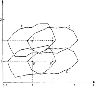
y ) segments are tested in the second part of the algorithm.

T h e numerical results, taken from Charles (1985), are shown in figure 8. T h e interesting point t o be noted is that the size of the ‘maximal’ sets given by condition (6.3) is already plausible from a practical point of view. Using condition (5.16) would yield still larger sets, with no basic increase in computational time. On the other hand,

0 3 1 2 a

Figure 8. ‘Maximal’ sets C obtained for example 1 around different nominal values ,t = ( d ,

On the uniqueness of local minima 433 the use of the much more restrictive condition (4.4) would lead, in this example, to a maximal set of the size of a point in figure 8, and it is thus inadequate for practical use.

7. Conclusion

We have studied the uniqueness of the local minima of general nonlinear least-squares problems, under the main hypothesis that the mapping to be inverted is regular C’ and has an injective derivative. For this case we have derived a sufficient condition that involves a minimisation, over all ‘geodesic’ curves of the image set, of a quantity that involves the radius of curvature of the ‘geodesic’ curve and a function related to the radius of curvature through the resolution of an elliptic problem (see (5.16)). This condition has been optimised among a class of possible sufficient conditions, but it is not known whether it is the best possible condition. However, numerical examples have shown that the proposed condition makes it possible to obtain practically interesting results for a two-parameter estimation problem.

References

Charles J-L 1985 Determination d’un domaine d e stabilite pour un prohlkme d’estimation d e parametres Rapport de D E A , Uniuersiii Puris-IX Duuphine

Chavent G 1983 Local stability of the output least square parameter estimation technique Mulkemuficu Aplicudu e Compuiutionul2 3-22

S p i e s J 1969 Eindeutigkeitsdtze hie der Nichtlinearen Approximation in Strikt-Konvexen Raumen Dissertation zur Erlangung des Doktorgrades Fachbereich Mathematik, Universitdt Hamburg (in German)