A Flow-Level Performance Model for Mobile Networks Carrying Adaptive Streaming Traffic
Texte intégral
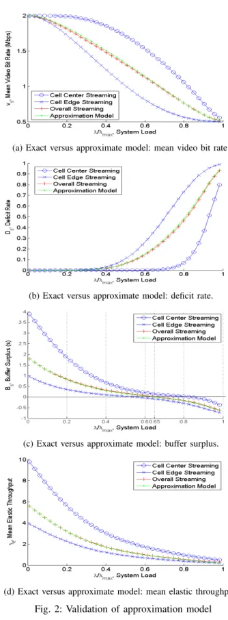
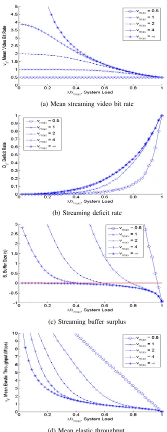
Figure

Documents relatifs
The short term implementation mechanism will use an ISO 8473 normal data PDU as the echo-request and echo-reply PDU.. A special NSAP selector value will be used to identify
If an S/MIME client is required to support symmetric encryption and key wrapping based on IDEA, the capabilities attribute MUST contain the above specified OIDs in the
When used in conjunction with MS-CHAP-2 authentication, the initial MPPE session keys are derived from the peer’s Windows NT password.. The first step is to obfuscate the
The problem list has been further analyzed in an attempt to determine the root causes at the heart of the perceived problems: The result will be used to guide the next stage
Additionally, there could be multiple class attributes in a RADIUS packet, and since the contents of Class(25) attribute is not to be interpreted by clients,
A Location-to- Service Translation Protocol (LoST) [LOST] is expected to be used as a resolution system for mapping service URNs to URLs based on..
When using "sms" URIs as targets of forms (as described in Section 2.6), the user agent SHOULD inform the user about the possible security hazards involved when
If the FA allows GRE encapsulation, and either the MN requested GRE encapsulation or local policy dictates using GRE encapsulation for the session, and the ’D’ bit is not
